The implication of the hyperbolic discount model for annuitisation decisions

City, University of London Institutional Repository

Citation: Chen, A., Haberman, S. ORCID: 0000-0003-2269-9759 and Thomas, S.

10.1017/S1474747218000343

This is the accepted version of the paper.

This version of the publication may differ from the final published

version.

Permanent repository link: http://openaccess.city.ac.uk/21116/

Link to published version: http://dx.doi.org/10.1017/S1474747218000343

Copyright and reuse: City Research Online aims to make research

outputs of City, University of London available to a wider audience.

Copyright and Moral Rights remain with the author(s) and/or copyright

holders. URLs from City Research Online may be freely distributed and

linked to.

The implication of the hyperbolic discount

model for the annuitisation decisions

November 24, 2018

The low demand for immediate annuities at retirement has been a long-standing puzzle. We show that a hyperbolic discount model can explain this behaviour and results in the attractiveness of long-term deferred annuities. With a set of benchmark assumptions, we find that retirees would be will-ing to pay a much higher price than the actuarial fair price for annuities with longer deferred periods. Moreover, if governments were to introduce a pre-commitment device which requires pensioners to make annuitisation decisions around ten years before retirement, the take up rate of annuities could become higher.

Keywords: Hyperbolic discounting, Deferred annuities, Annuity puzzle, Reservation price.

1 Introduction

Over the past few decades, the traditional defined benefit (DB) pension plan has been gradually losing its dominance in private sector pension systems in many countries and the defined contribution (DC) pension plan has become increasingly popular (OECD, 2016). Under the DC pension scheme, members contribute towards their personal pen-sion savings in a way that enables them to make decipen-sions on how to invest during the accumulation stage and how to decumulate during retirement.

illustrated by low levels of voluntary annuitisation in the UK market. In the past, the UK had two distinct annuity markets: a voluntary segment called the Purchased Life Annuity (PLA) market and a compulsory section called the Compulsory Purchase Annuity (CPA). Based on UK annuity sales figures for the 1994-2006, sales in the CPA market had been consistently higher than that in the PLA market. By 2010, the CPA market had grown to £11.5 billion worth of annuity premiums while the PLA market only had £72 million worth of sales (Cannon & Tonks, 2011).

Recently, the UK government implemented pension reforms to encourage free choice of the mode of pension distribution and, as a result, retirees’ real preferences on annuity products could be clearly seen. The reform follows the international trend of greater pension flexibility, which has been observed in countries such as the USA, Australia and Switzerland. Prior to the 2014 UK reform, there were strict restrictions on accessing pension savings at retirement. For example, if a pensioner had overall pension savings of greater than £18,000 but could not access a guaranteed retirement income of more than £20,000 per year1, the only two choices that they could make were to either to buy an annuity or enroll in a “capped drawdown”, which allowed them to withdraw as much as 120 percent of an equivalent annuity each year during retirement. However, after the 2014 policy change, everyone is able to choose a lump sum (full withdrawal), an annuity or a drawdown, regardless of the size of their pension wealth (HM Treasury, 2014). With this move towards greater freedom of choice on how and when to access pension wealth, annuity sales have experienced a large decline. In Q2 2015,£990m was invested in annuities, showing a 44 percent decrease from the £1.8bn invested in Q2 2014. Moreover, 18,200 annuities had been purchased in the three months after the pension reform, showing a 61 percent decrease compared to Q2 2014 when 46,700 were purchased (ABI, 2015).

Many studies have suggested a number of reasons for the annuity puzzle, such as mortality risk-sharing among families (Brown & Poterba, 2000) and the existence of social security (Butler et al., 2016). Some research has examined the possible influences of behavioural factors such as the framing effect, cumulative prospect theory and low level of financial literacy; the findings suggest that the low demand for annuity could be simply due to irrational behaviour (Cannon & Tonks, 2008). In the next Section, Literature Review, we will provide a more detailed explanation of the reasons.

Since the annuity is a product that involves a series of payments at different points of time, one of the behavioural factors that affects decision making is the inconsistency of intertemporal choices. More specifically, when people assign values to future payouts, the discount rate used to evaluate intertemporal choice is not fixed, but varies in line with the length of the delay period, size and signs of the benefits. This effect is called hyperbolic discounting and is interpreted as “temporal myopia”. The concept has been widely used to account for behavioural bias in savings, nutrition, healthcare, drug addictions, and other problems of willpower (Frederick et al., 2002). Laibson et al. (2003) have used the model to explain the puzzle of simultaneously having large credit card debts and

1

A guaranteed retirement annual income of£20,000 is equivalent to a total pension savings of around

pre-retirement savings.

In this paper, we use the hyperbolic discount model derived from experimental results to analyse annuitisation decisions. In section 3, we provide a full explanation of the model and suggest how to apply the model in valuing annuities. In terms of the prod-ucts considered, we are interested in both immediate annuities and deferred annuities. The deferred annuity is a contract that is purchased today but does not pay until the annuitant survives to a pre-specified age. Compared with a conventional immediate an-nuity, a deferred annuity has competitive advantages of a much lower price and provides almost the same level of longevity insurance; therefore, it has aroused much discussion in the area of retirement financial planning (see Milevsky, 2005; Gong & Webb, 2010; Denuit et al., 2015). To uncover the annuitisation decisions of people at different ages, two types of deferred annuities are studied: a working age deferred annuity (WADA), which is purchased at working age and starts paying at retirement, and a retirement age deferred annuity (RADA), which is purchased at retirement and starts paying a few years later. To be more specific, we seek to explore four questions:

1. Can we use the hyperbolic discount model to explain the low demand for immediate annuities at retirement and at a more advanced age?

2. Are pensioners at 65 years old interested in purchasing a RADA?

3. Would people at working age have an interest in purchasing a WADA (with a single premium or with regular premiums)?

4. How would working-age members respond to a question asking them to decide today whether to buy an immediate annuity at retirement?

To seek the answers to these questions, we adopt the hyperbolic discount model to evaluate the perceived value of an annuity, which enables us to work out the reservation price. By comparing the reservation price with the theoretical market price we can determine whether an individual would choose an annuity or not. We show that time inconsistent preference is one of the factors that stops retirees from converting their DC account balances into annuities at retirement. More importantly, we identify a high willingness to purchase long-term deferred annuities for hyperbolic discounters, both at working age and in retirement. As the deferred period increases, the relative difference between reservation price and actuarial price increases considerably and at a much faster rate. Furthermore, if members are simply asked to make a decision on annuity purchase and could delay the action until the point of retirement, those with around ten years until retirement value the longevity protection the most.

2 Literature review

Yaari (1965) is the first to demonstrate the benefits of annuitisation in a life cycle model with an uncertain lifetime. He shows that a rational investor should invest his retirement savings in annuities rather than bonds to finance retirement. This result rests on three fundamental assumptions: a complete annuity market, a specific utility function (having the property of additive separability) and the absence of a bequest motive. The subsequent literature on annuities has relaxed one or two of these assumptions in order to assess if these factors lead to the low demand for annuities.

Annuities in a rational framework

Observing the annuity market from the supply side, a less competitive price could be the reason for low demand. Brown & Warshawsky (2001) calculate the money’s worth value of an annuity using average mortality rates of the population and find that an individual could expect to receive only 85 pence per pound invested, thus justifying the existence of adverse selection in annuity pricing.

Since an annuity stops paying once the annuitant dies, people with a motive to be-queath part of their wealth obtain less welfare by purchasing a life annuity. A large literature has focused on how the bequest motive impacts the demand for annuities and shows that a strong bequest motive can eliminate the desire to purchase annuities (see Friedman & Warshawsky, 1990; Vidal-Melia & Lejarraga-Garcia, 2006; Lockwood, 2012). Intra-family mortality sharing can also be regarded as a substitute for an annuity. Since families often share a common budget constraint, mortality risk sharing among family members can offer a substitution for risk sharing in the annuity market. To an extent, this resembles the bequest motive; an individual who dies early leaves his wealth to subsidise other family members who are alive. Brown & Poterba (2000) find evidence showing that the utility gain from annuitisation for a couple is significantly lower than that for single people.

An alternative explanation for the low demand for additional annuitisation is the existence of social security and private DB pension plans. According to Dushi & Webb (2004), an exceptionally high proportion of a retired household’s wealth has been pre-annuitised before retirement. Therefore, without purchasing an annuity in the open market, these retirees already have a minimum level of income that will last for life. Butler et al. (2016) also prove that the presence of social security reduces the value of annuitisation.

A more recent discussion relates to the worry about health care expenditure shocks at an older age and the fact that retirees may not need the smooth consumption that an annuity provides. It is true that people have a higher probability of falling ill when they become older; they may also have to make some age-specific investments in a house such as installing a stair lift. Therefore we have reason to believe that a rational retiree might want to live a very simple life in their early retirement period so that they can save for unexpected health-related expenses (Sinclair & Smetters, 2004).

the alternative of never annuitising, in practice, a retiree can choose between annuitising now and delaying the decision until the next period. They can also annuitise only a fraction of their wealth and enter a drawdown of the rest. Gavranovic (2011) has demonstrated that the optimal annuitisation strategy for a pensioner without bequest motive is to gradually convert all pension wealth to annuities by around age 80.

Annuities in a behavioural framework

The literature mentioned above seeks to solve the annuity puzzle within a strictly rational framework. In recent years, however, there is an extensive literature on the behavioural economics of retirement savings. This moves beyond the fully rational paradigm and proposes some behavioural factors that could play important roles in determining how retirees spend their retirement savings.

One important issue is the flaws in the expected utility hypothesis that arise from risk aversion. Hu & Scott (2007) have explained the annuity puzzle by assuming that retirees are loss-averse rather than risk-averse, and make annuity decisions based on Cumulative Prospect Theory (Tversky & Kahneman, 1992). They also extend the application of Cumulative Prospect Theory to deferred annuities and guaranteed annuities, showing that the deferred annuity becomes optimal only when the first payment starts on or after age 93.

Another behavioural factor, the framing effect, which states that individuals’ be-haviour depends heavily on the way in which available choices are presented, is also shown to be one of the influencing factors by Brown et al. (2008). They have shown that 72 percent of subjects prefer an annuity rather than a savings account when the choice is framed in terms of consumption while 12 percent subjects choose an annuity when it is framed in terms of an investment.

Moreover, Brown et al. (2012) show that it is difficult for people to make decisions when choices are very complex and not repeated. The annuity is one example of a complex financial product and the observed low level of annuity purchases may be explained by this.

As annuity products involve a series of payments that come in the future, we be-lieve that behavioural factors that affect discounting methods would influence annuity valuations, and hence annuity purchase decisions. Laibson (1998) has used hyperbolic discount models to explain a wide range of empirical anomalies, such as consumption discontinuity at retirement and under-saving. In this paper, we use this model to study annuitisation decisions. In the next section, we give a detailed explanation of the hyper-bolic discount model.

3 An introduction to the hyperbolic discount model

rate is constant over time and is independent of money amounts (or utilities). This often leads to a conclusion that individuals’ preferences are stationary over time, i.e. they have time-consistent preferences. In the real world, many empirical studies have observed anomalies in actual behaviour compared with what is predicted by the expo-nential discount function. Three major anomalies have been found. First, people tend to act impulsively in the short-term but become more patient in the long-term. In other words, the implicit rate at which people discount future rewards will vary inversely with the length of waiting time. Thaler (1981) illustrates this with a simple example. Sub-jects are asked to state their preferences on two questions: “Would you prefer one apple today or two apples tomorrow?” and “Would you prefer one apple in one year or two apples in one year plus one day?”. According to the exponential discounting method, people who choose one apple today should make consistent choice of one apple in a year. However, empirical results show that a significant fraction of subjects that prefer one apple today would gladly wait one extra day in a year’s time in order to receive two apples instead. Second, the implicit discount rates with regard to different reward sizes would not stay the same. Thaler (1981) finds that the subjects are indifferent between receiving $15 immediately and $60 in a year, between $250 now and $350 in a year, and between an immediate $3000 and $4000 in a year, which means large reward sizes have lower discount rates compared with small reward sizes. Third, there is a gain-loss asymmetry in terms of discounting. For example, Loewenstein (1987) finds that a group of subjects, on average, are indifferent between receiving an immediate $10 and receiving $21 in a year; but are indifferent between paying $10 immediately and paying $15 in a year. Similarly, the indifferent amount for receiving or paying an immediate $100 were receiving $157 or paying $133 respectively in a year.

The anomalies introduced above can be addressed by a hyperbolic discount model, which has been widely applied to explain the problem of addiction and self control. As an example, people with low self-control often find it difficult to improve their health by doing more exercise and having a diet. These people often pre-commit to forgo all future temptations, in exchange for improved health in the future; however, when they have their next meal, they cannot resist having unhealthy food and desserts (Redden, 2007). Presumably, they prefer this because the instant pleasure delivered by delicious food is greater than the heavily discounted future rewards of health. Therefore, the hyper-bolic discount model is appropriate to describe the situation that people simultaneously require immediate satisfaction and make commitments for the future.

Loewenstein & Prelec (1992) collectively present the experimental evidence and pro-pose an explicit hyperbolic discount model to address the effect.

δ(t) = (1 +αt)−αβ withα >0, β >0 (1)

where δ(t) is a discount function; α and β determine how much the function departs from constant exponential discounting.

indifferent relative to a certain gain at the current time; Abdellaoui et al. (2009) elicit different time weights by varyingt. Relying on their results, we use the “Power discount model” where α = 1 so that δ(t) = (1 +t)−β in our analysis; here the best estimate β equals 0.19 for gains and 0.11 for losses. Please note that value of β would vary with country/cultural background of the selected group of subjects and the limitation is embedded in the experimental design. Therefore, in section 6, sensitivity to the parameter β is explored, to show that the conclusions do not entirely depend on the chosen values of the parameters.

Figure 1 here

Figure 1 provides a comparison between the hyperbolic discounting and exponential discounting models. The horizontal axis represents the waiting time to receive £1 and the vertical axis is the present value of the£1 to be received. The present value following hyperbolic discounting decreases at a much faster rate in early years than following expo-nential discounting, which means that the hyperbolic discounters adopt a higher level of discounting for benefits that come in the early years than exponential discounters. How-ever, if the benefits are to be received after 20 years (the intersection point), hyperbolic discounters believe that they have a higher value than exponential discounters.

In addition to the discount function, a descriptive value function is also required in a complete discounted utility framework. Loewenstein & Prelec (1992) discuss the neces-sary characteristics of the value function without providing an explicit descriptive model. Abdellaoui et al. (2009) design a parameter-free measurement of value in intertemporal choices and hence derive the value function which addresses the absolute magnitude ef-fect and the gain-loss asymmetry. In deriving this function, Abdellaoui et al. (2009) do not specify the form of the utility model in the beginning; however, they construct the shape of the value function from the experimental results2. After that, they find that the model below (in Equation (2)) can provide the best fit to the shape of the value function; and they estimate the parameter values. The value function v(ct) is given below with

γ being equal to 0.97 andθ being equal to 0.84. This function is concave for gains and convex for losses, reflecting a property of “diminishing marginal sensitivity”. This value function is assumed to be separable and additive over time as recorded in the literature.

v(ct) =

−(−ct)γ ifct<0

cθ_t ifct≥0

(2)

where ct represents the consumption rate that would take place at a future time t,

which is defined on the interval [0,T], andv(ct) represents the value of the consumption

amount.

The discount rates and the value function are combined to arrive at the overall value

2

of consumption streams.

V(c0, c1, ..., cT) = T X

t=0

(δ(t)×v(ct)) (3)

A standard approach in the literature has been to use the exponential discount model forδ(t) and an utility function, for example Constant Relative Risk Aversion (CRRA), forv(ct). In this analysis, we instead use the hyperbolic discount model in Equation (1)

and the corresponding value function given by Equation (2) to analyse annuity purchase decisions. We therefore are able to analyse the effect of subjective views on the underlying consumption streams.

4 Annuity Valuation

In this section, we introduce four scenarios to address the questions of annuitisation decisions for people at different stages. Two types of annuities, immediate annuities and deferred annuities, are discussed in this paper and they are priced at actuarially fair rates. In order to make a fair decision, the overall utility, V, of the investment in each scenario will be calculated. As we focus on people who show “temporal myopia”, the amount of money is evaluated based on Equation (2) and time preference is modeled by the “power discount model”, Equation (1) with α = 1. Let tpx denote the probability

that anx-year-old person can survive fortyears and the maximum attainable age is set to be 120. Four scenarios are described in detail below and the corresponding valuation of the annuity investment is introduced.

a. Immediate annuities for retirees

Consider a retiree at age x(x≥65) who needs to make a decision on whether to spend a lump sum amount A to purchase an immediate annuity which pays ψ per annum in advance. The overall value of this investment for the x-year-old is:

V1(x) =v(−A) + 119

X

i=x

(δ(i−x)×i−xpx×v(ψ)) (4)

b. RADA for retirees

V2(d) =v(−A) + 119

X

i=65+d

(δ(i−65)×i−65p65×v(ψ)) (5)

c. Working Age Deferred Annuity (WADA) for working age individuals3

An individual at age x (25≤ x ≤ 64) considers investing in a WADA which provides annual incomes of ψ once the annuitant survives to retirement age 65. Either a single premiumA(at agex) or a series of regular premiums (spreading between age xand age 65) is required. The overall perceived value of this investment at the time of purchase is (below we show the formulae of the case with a single premium):

V3(x) =v(−A) + 119

X

i=65

(δ(i−x)×i−xpx×v(ψ)) (6)

d. Decision on purchasing an immediate annuity at retirement for working age individuals

In this scenario pension scheme members within the working age range (25≤ x ≤64) are asked to make decisions in advance on whether to choose a pension lump sum A at age 65 or a corresponding fair annuity starting at the same age. When evaluating this annuity, the cash flows involved are exactly the same as the immediate annuity purchased at age 65 (Scenario a); however the perceived value may be different because the decision is made at an earlier age. If an individual decides to convert the lump sum A into an annuity at retirement, the overall perceived value of this investment for the individual is:

V4(x) =δ(65−x)×65−xpx×v(−A) +

119

X

i=65

(δ(i−x)×_i−xpx×v(ψ)) (7)

To determine whether an actuarially fairly priced annuity is attractive to purchase, we follow Hu & Scott (2007) to use the “relative difference between reservation price and fair price”,R, as the benchmark measure:

R= Reservation P rice−Actuarially f air price Actuarially f air price

The “reservation price”, also called the “maximum acceptable price”, is the annuity price that would make an individual indifferent to buying an annuity. According to the valuation functions above, the reservation price is the initial price, A, that makes the hyperbolic present value of an annuity, V, equal to zero. If the reservation price is below the market price, the annuity would not be attractive for individuals to buy.

3_{The working age deferred annuity was a common product that was offered in the UK in the past.}

Therefore, a positiveRmeans individuals are willing to purchase a fairly priced annuity, and a higher value ofR implies greater willingness to purchase an annuity. R can also be interpreted as the percentage more or less than the market price that an individual would be prepared to pay for a product.

5 Results

In this analysis, we assume the annuity price is actuarially fair with no expenses or profit loading. The price calculation is based on the UK mortality table “S2PML4_”, which describes the mortality experience of UK male pensioners of self-administered pension schemes for the period from 2004 to 2011, and a constant interest rate of 3 percent. Annual income from annuity, ψ, is assumed to be 1 unit. Therefore, the fair market price of the annuity and the reservation price that individuals would like to pay can be calculated accordingly. In what follows, we provide results for the relative price differences, R, under the four different scenarios, analyse the attitudes of investors to-wards each type of annuity and discuss the relation between the relative price differences and investors’ age or the length of the deferred period.

a. Immediate annuities for retirees

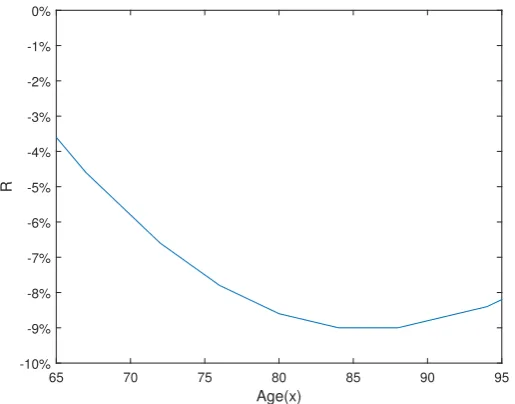
The results of the Relative Price Differences (R) with regard to different ages of purchase are presented in Figure 2. Two major conclusions can be drawn from the figure. First, all the outcomes in terms of R are negative, which means that for a group of retirees who are aged between 65 and 95, fairly priced immediate annuities are unattractive to purchase. Thus, evaluating annuitisation decisions by assuming time inconsistent preferences is indeed a powerful behavioural explanation for retirees’ not converting their defined contribution account balances into annuities. Secondly, as a newly retired pensioner becomes older, his preference for the immediate annuity declines at first and then increases after he reaches age 85. However, the relative difference in price is small withR lying in the range of −3% and−10%.

The results presented appear to be inconsistent with recent research carried out by Schreiber & Weber (2015), who find that the expected present value of an immediate annuity declines monotonically with the age of purchase. Although both studies use the power discounting model for annuity evaluation, different groups of people are targeted: Schreiber & Weber (2015) survey working age individuals while we focus on retirees above age 65; and this may explain the inconsistency.

Figure 2 here

b. Retirement Age Deferred Annuity (RADA) for retirees

Figure 3 shows the attractiveness of RADA with different deferred periods for a 65-year-old retiree. It can be seen that although recently-retired individuals are reluctant

to purchase immediate annuities, they are willing to pay a higher-than-market price for annuities with long deferred periods. From our modeling results, annuities that are deferred for more than 10 years are generally welcomed by 65-year-old retirees. Furthermore, we identify a positive relationship between the length of the deferred period and the attractiveness of the corresponding deferred annuity. If an annuity has a deferred period of 30 years, a 65-year-old individual would be prepared to pay 24% more than the fair price5.This is a much higher margin than that for an immediate annuity. It implies that such a product would have commercial potential since insurance companies could add a greater loading in the pricing of deferred annuity products without changing their attractiveness.

The popularity of deferred annuities have also been identified in other work. Hu & Scott (2007) adopt Cumulative Prospect Theory (CPT) to evaluate deferred annuities with deferred periods of 0, 10, 20 and 30 years and find that the 30-year deferred annuity is the most attractive to buy. In Chen et al. (2018), we also show that the attractiveness of a deferred annuity increases with the length of the deferred period, according to CPT.

Figure 3 here

c. Working Age Deferred Annuity (WADA) for working age individuals

If individuals at working age are given the opportunity to enter a deferred annuity contract that promises retirement incomes depending upon survival, their reactions are examined and reflected in Figure 4. It can be seen that although people who are retired are unsure of handing over a lump sum of money to insurance companies in exchange for longevity protection, most people at working age tend to find a WADA attractive to buy. Another interesting point worthy of note is that the decision maker’s age has a negative effect on the attractiveness of this type of deferred annuity. For hyperbolic discounters younger than 30-year-old, they appear even to be willing to pay double the price of the WADA.

Figure 4 here

We know that as the length of deferred period increases, the actuarially fair price of a deferred annuity which provides the same level of protection becomes cheaper; hence younger individuals would be less hesitant to purchase a WADA which involves a smaller initial outlay. In addition, given the assumption that people have time inconsistent pref-erences, a young individual tends to overvalue all of the annuity incomes that come in the distant future; however for an older individual, some of the deferred annuity payments are highly likely to be undervalued. The results are consistent with our conclusions in Scenario b. Purchasing the pension annuities at an earlier age means a longer deferred period, and in both scenarios an annuity with a longer deferred period is more attractive.

5

The magnitude of R is much higher in Scenario c than in Scenario b because a longer deferred period is considered.

The major conclusions regarding WADA also hold when we allow the deferred an-nuity premiums to be spread over the entire deferred period. Being aware that young individuals might not have enough savings to afford the lump sum premium to enter the WADA contract, or a large lump sum to be paid years before receiving any benefits might decrease the marketability, we consider the situation when premiums are to be paid annually in advance between the age of purchase and the retirement age. If they die before the retirement age, no premiums would be returned; otherwise they would start receiving annuity payments from age 65 until the point of death. The results of the Relative Price Difference (R) is shown in Figure 5. It again shows that most people at working age (below age 60) would find a WADA attractive to buy; and the decision maker’s age has a negative impact on the attractiveness of WADA6.

Figure 5 here

Some of our findings mirror those suggested elsewhere. Shu et al. (2016) have con-ducted a choice-based stated-preference survey of adults aged between 45 and 65 and find that younger subjects report a higher likelihood of purchases for annuities beginning at age 65 than older subjects who are closer in age to the start date. DiCenzo et al. (2011) have also discovered that pre-retirees have stronger preferences for annuities than retirees based on online experimental research with 1,009 subjects aged between 45 and 75.

d. Decision on purchasing an immediate annuity at retirement for working age individuals

Similar to the third scenario, we aim to discover the attitude of working age pension scheme members towards an annuity with the first payment starting when pensioners retire at age 65. Although the annuity investment payoffs are exactly the same, the purchase is made at different points. In Scenario c, the price is paid now at agex while in Scenario d, pensioners simply make a decision at agexbut delay the purchase action until age 65. If an individual dies prior to the time of retirement, his financial status remain unchanged in Scenario d but he faces an absolute loss of the price paid in Scenario c. Therefore, Scenario d effectively deals with the decision to buy an immediate annuity rather than a deferred annuity.

6

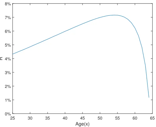
Comparing the results ofR in Figure 6 with those in Figure 4, we identify a different pattern. For individuals below age 55, the attractiveness of the annuity increases slightly with age. However for individuals above age 55, the attractiveness declines sharply with age and becomes unattractive when individuals reach age 65. We notice that the occurrence of the kink is due to the different discounting parameterβfor gains and losses. When the discounting parameter values for gains and losses are set to be the same, the kink disappears and the attractiveness reduces with the waiting period (time point of decision and retirement age)7. In future work we would look into the differences in the gain loss discounting, and test how sensitive our results are to the gain-loss asymmetry. With the results indicated by Figure 6, we suggest that policy makers who want to promote annuitisation in public ask individuals to make a choice between lump sum and annuities around 10 years before retirement. On the other hand, one may notice that the change in R is relatively small, varying between 4% and 8%. It is similar to the results for immediate annuities in Scenario a.

These findings confirm those in the survey by Schreiber & Weber (2015). In their survey, subjects are asked to predict whether they will annuitise if they were at age 66. The total sample results show that the effect of age on the decision to purchase an annuity is negative. However, observing the answers from a subsample of individuals below age 51, the effect is no longer statistically significant. To some extent, it reveals that people above age 51 have significant decreasing preferences towards annuities.

Figure 6 here

6 Sensitivity analysis

Previously, we assumed that each parameter value in the annuity calculations is based on the work of Abdellaoui et al. (2009). However, questions remain as to whether the behavioural biases would be stronger or weaker for people with different levels of impatience, different income levels or different health status. In this section, we test the sensitivity of the interest rate, the power discounting parameter, the value function parameter, the income levels and mortality rates (by changing mortality tables).

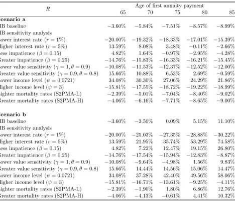
Table 1 shows the results for Rin Scenario a and Scenario b under different combina-tions of assumpcombina-tions. The row HB baseline lists the standard results that are based on the benchmark assumptions in Abdellaoui et al. (2009). In the HB sensitivity analysis, we change one factor listed in each row at a time so that we can observe the impact of that factor on R. “Less” or “greater” is relative to the baseline results. Each column represents different types of annuity products with the first payment starting at a dif-ferent age. For example, an annuity starts paying at age 75 represents an immediate annuity purchased at age 75 in Scenario a and a 10-year deferred annuity purchased at age 65 in Scenario b.

Table 1 here

The first factor that is of interest is the interest rate, which is an important factor in pricing an annuity. As the interest rate moves from lower (r= 1%) to higher (r= 3%), R consistently increases, for all types of immediate annuities and deferred annuities. This feature is simply because a higher interest rate leads to a lower annuity price, which helps investors lock in a high rate of return. For immediate annuity purchasers (Scenario a), it is better to choose an annuity starting at age 65 when the interest rate is high; however, it is better to delay the purchase when the rate in the market is low. For deferred annuities (Scenario b), the interest rate is of less concern compared with immediate annuities (because a smaller number of payments will be discounted). The attractiveness of the deferred annuity will depend on the relative level of patience of investors. For an individual with a certain level of impatience, they tend to overvalue future benefits more heavily when the interest rate is higher. Therefore the longer-term annuity becomes more attractive in a high interest rate environment.

Another factor that we investigate is the level of impatience, measured by β. Given that the annuity pricing rate is deterministic, a higherβ means that the decision maker adopts a heavier undervaluation of earlier benefits and a lighter overvaluation of later benefits. Reflecting on the curves in Figure 7, the intersection point between exponen-tial discounting and hyperbolic discounting would come at a later stage as β increases. Comparing our baseline results with less/greater impatience for both immediate annu-ities and RADA, we conclude that the attractiveness of annuity products is consistently lower in response to a greater level of impatience. This makes sense intuitively since an individual with a greater level of impatience would have stronger present bias; they would gain much higher satisfaction from consuming now rather than converting the lump sum into future cash flows and consuming regularly. According to Table 1, rel-atively patient individuals (β = 0.15) are willing to pay a slightly higher price, 4.82% and 1.64% respectively, for immediate annuities at age 65 and 70. It is because they are patient to wait and assign more weight to future incomes. Investment opportunities that convert current consumption into a future stream of cash flow are attractive to them. The same reasons lead to the attractiveness of deferred annuities for this group of people (see the row corresponding to β= 0.15 in Scenario b).

Figure 7 here

The effect of annuity income levels is examined to capture the variation in decisions of people with different wealth levels. Two levels of annual income, 0.07218 unit and 3 units, are adopted to represent relatively poor people and relatively rich people. Based on the value function in the hyperbolic discount model introduced above, people tend to overvalue the amount of less than one unit and undervalue the amount of greater than one unit. This is reasonable since people often place more values on the initial accumu-lation of an amount of money and this portion of money is intended for the purchase of necessities such as food, utilities and rent. Therefore, the results corresponding to ψ= 0.0721 and ψ= 3 in Scenario a and Scenario b show that relatively wealthy people who can afford an annuity with higher annual incomes are willing to pay a lower-than-market price, while relatively poor people are willing to pay a much higher-than-lower-than-market price for annuities.

The mortality sensitivity analysis is conducted by comparing results from two mor-tality tables: S2PMA-L, the mormor-tality experience of male pensioners with high pension amounts and relatively lower mortality rates, and S2PMA-H, the mortality experience of male pensioners with low pension amounts and relatively higher mortality rates. Results in Scenario a show pensioners with the highest mortality rates (S2PMA-H) tend to find immediate annuities the least attractive. Similarly, those with low mortality rates and long life expectancies (S2PMA-L) show the greatest interest in RADA, as is observed in Scenario b.

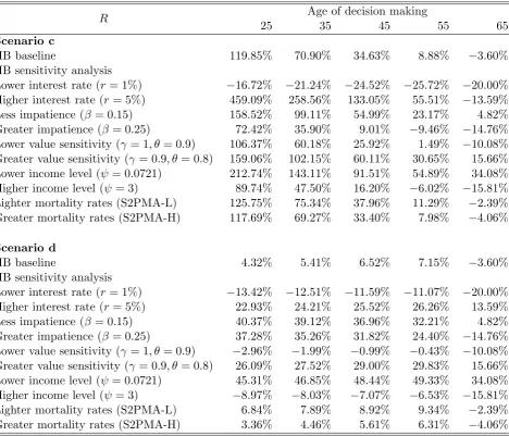
Table 2 shows the results in terms of R in Scenario c and Scenario d. In Table 2, we can see the sensitivity of four factors: the interest rate, the level of impatience, the value sensitivity, the level of income and mortality rates, on the annuitisation decisions.

Table 2 here

The sensitivity analysis of the interest rate in Scenario c and Scenario d again shows that annuities are generally attractive in a high interest rate environment. Moreover, as the deferred period increase, the increase in attractiveness (R) is greater when the inter-est rate is higher. As explained previously, the reason behind this is that an individual with a certain level of impatience would overvalue future benefits more heavily when the interest rate is higher. When the deferred period is greater than a certain number of years, it is possible that all payments will be overvalued.

By comparing results corresponding to β = 0.15 and β = 0.25, we find those at working age see annuities as more valuable when they experience less impatience. In addition, for decision makers with different levels of impatience, the effect of their age on the WADA’s attractiveness is consistently negative. In other words, the longer the waiting period to receive the first annuity income is, the higher the possibility of purchase will be. The intuition behind these features is as follows: incomes that arrive further in the future are more likely to be overvalued and thus the deferred annuity with a longer waiting period has a higher maximum acceptable price.

8

The results with different levels of value sensitivities in Scenario c and Scenario d reinforce our conclusions drawn from Table 1. In general, deferred annuities are more attractive when the deferred period is longer. A greater underestimation of losses would make the deferred annuities even more attractive. We note that the underestimation of gains also has an impact on the results, however the impact (for example θ changing from 0.9 to 0.8) is much less significant than that of the underestimation of losses. This feature occurs because our model considers a one-off lump sum premium payment for entering an annuity contract.

In Scenario d where the real purchase of an immediate annuity is delayed until re-tirement, we have shown in the baseline results (which assume that β is 0.19 for gains and 0.11 for losses in the power discount function) that people have the greatest interest in buying an annuity around age 55. However in the sensitivity analysis when we let discount rates for gains and losses be the same, the peak in the trend of R disappears and we see a gradual decrease of value of R relative to the age of decision making. In such a case, governments may simply encourage individuals to make annuitisation decisions earlier rather than 10 years before retirement. Whether people use different discount rates for gains and losses and the resulting impact on annuitisation decisions needs future research.

Results corresponding to ψ = 0.0721 and ψ = 3 in Scenario c and Scenario d show that wealthy decision makers who can afford an annuity with a high annual income tend to find annuities less attractive. The impact of income levels on the annuity purchasing behaviour are consistent for decision makers at all ages9.

The sensitivity of mortality rates in Table 2 indicates intuitively that annuities are more attractive for individuals with longer life expectancies, regardless of the age of decision making and the age of annuity purchase. Furthermore, for different mortality groups, age presents a negative influence on the attractiveness of a WADA. If the an-nuitisation decision needs to be made at working age and the actual purchases could be delayed until retirement, those between 50 and 55 are the most likely to choose an annuity and a strong decline in annuity preferences exists for pensioners older than 55. In order to measure the responsiveness of the Relative Price Difference to the change in each parameter, we calculate the elasticity of the Relative Price Difference, ER. It

addresses the percentage change in the Relative Price Difference for a given percentage change in the parameter value and the formula is as follows:

ER=

Percentage change inR

Percentage change in parameter value =

4R Raverage

4parameter parameteraverage

(8)

In Equation (8), 4R stands for the absolute change in R and 4parameter stands for the absolute change in the considered parameter values. Raverage stands for the absolute value of average of R under different parameter values andparameteraverage is the absolute value of the average of chosen parameter values. As the average value is used to calculate the percentage change, the elasticity of the Relative Price Difference

9

can be regarded as a point mid-way among all of theRresults. After we calculateERfor

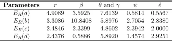
each immediate annuity or for each deferred annuity, we average the results and obtain the elasticity of the Relative Price Difference for annuities in four different scenarios. The results are presented in Table 3. Please note that we use life expectancy at the age of annuity purchase as an index for each mortality table.

Table 3 here

If ER is greater than 1, the Relative Price Difference changes proportionately more

than the parameter value changes. If ER is less than 1, the Relative Price Difference

changes proportionately less than the parameter value changes, implying a less sensitive parameter. Based on the results in Table 3, the following conclusions can be drawn. First, the interest rate is a very sensitive factor in influencing annuity purchase decisions, especially immediate annuity purchase decisions. This is reasonable as the interest rate is one of the most important annuity pricing factors. For immediate annuity products that requires a large initial payment, a small change in interest rate can change premium greatly. Second, the Relative Price Difference is responsive to a small change in the level of impatience, which is measured byβ. It confirms our findings in the sensitivity results of Table 1 and 2 that people with different levels of patience would hold distinct opinions regarding the purchase of annuities. Third, the Relative Price Difference is very sensitive to the parameter values of the value function; and the sensitivity is more significant for immediate annuity products than for deferred annuity products. This is due to the property of “diminishing marginal sensitivity”, the deviation of the perceived value from the real value would be more significant for an annuity product with a higher price. Fourth, deferred annuities have greater sensitivity to mortality parameters than immediate annuities. This is partly due to the fact that incomes generated from the deferred annuities will be delayed for a few years; hence there is a possibility that the annuitant would not receive any incomes should they die during the deferred period.

7 Conclusions

Although purchasing an annuity at retirement can guarantee lifetime incomes, people are reluctant to spend their retirement savings on annuities voluntarily. In the UK, with fewer restrictions on accessing retirement savings, the demand for annuities has decreased and thus insurance companies are making efforts to design more attractive annuity products. This paper discusses the implications of one behavioural factor, time inconsistent preferences (as represented by the hyperbolic discount model), on the an-nuity purchasing decision.

Based on the analysis, we have the following primary findings. First, for an 65-year-old retiree, the reservation price of an immediate annuity is lower than the market price, and thus the hyperbolic discount method captures the low demand for annuities at retirement, as seen in practice.

deferred period. For instance, those below the age of 30 would pay more than double the market price for the WADA. However, our model does not account for factors such as affordability, a liquidity requirement and expected retirement living standards. While a 25-year-old man who wants to receive an annual annuity income of £40,000 after retirement might find a 40-year deferred annuity attractive; he will most probably not be able to afford the annuity price of£150,034.610at this young age. With time passing, he will accumulate wealth and set aside a portion for retirement protection. Often, there will be a point when accumulated retirement savings equal the deferred annuity price; this is the optimal age of purchase. Alternatively, a more affordable plan is to choose regular premiums spreading over the period between current age and retirement age. We have shown that the positive relationship between attractiveness and the deferred period is maintained under this scenario of regular premiums.

We recommend using the deferred annuity contract as a retirement solution because it requires a smaller initial investment than the immediate annuity and provides similar longevity insurance. In addition, based on the fact that analytical cognitive function ability declines dramatically for older adults, it would be wise to buy a RADA to protect consumption at very advanced ages. For those in their 80s, it has been shown that 20 percent have fully diagnosed dementia and 30 percent have severe cognitive impairment; and thus, it would be difficult for these individuals to make rational withdrawal decisions if there were no income protection in place (Laibson, 2009).

Currently when the public has limited knowledge on deferred annuities, a policy recom-mendation we would like to draw is to introduce compulsory annuitisation with respect to deferred annuities. The significant decrease in annuity sales after the pension reform may cause unforeseeable social problems in future especially for those who have limited financial knowledge to manage pension savings effectively and wisely. Although we sup-port the idea of flexible choices in pensions arrangements, we believe that the annuity product’s main function of providing longevity risk protection should be retained to some extent. Overall, making the deferred annuity purchase a compulsory choice would have the following benefits. First, it can protect individuals against myopia, and protect governments from potential increasing expenditure on social benefits. Second, it would encourage life insurance companies to enter the market and start offering deferred an-nuity products. Third, a compulsory policy helps to reduce or remove adverse selection, which is of vital importance in insurance markets. A reduced degree of adverse selection would ensure a large efficient market, and it would mean that annuitants are more likely to receive close to 100% of the fair annuity value.

In Scenario d, we observe that individuals around the age of 55 are those who would most likely commit to buy an immediate annuity at the point of retirement. Relying on this result, another policy recommendation can be drawn. With the aim of promoting the purchase of annuities among retirees and releasing the burden from social benefit claiming, governments are advised to introduce a pre-commitment device asking people

10_{The price is the actuarially fair annuity price based on assumptions of 3% annual real rate of return,}

to make annuitisation decisions around 10 years before retirement. When they reach retirement, their original decisions could be changed but some efforts, such as making a phone call or writing a letter, are required. In fact, in Denmark, the decisions on annuity purchases can be made during the accumulation period. As a result, about 50 percent of defined contribution assets are used to buy WADA type products for those aged in their 40’s, 50’s and 60’s (Andersen & Skjodt, 2008).

In the sensitivity analysis, we have explained that the optimal point of age 55 is due to different discounting parameter values used for gains and losses. The kink would disappear if we were to assume the same discounting factors for gains and losses. In future work, we would like to look into the area of gain-loss discounting asymmetry and examine more detailed impacts on our conclusions.

It is worth mentioning that currently the deferred annuity products (WADA and RADA) do not exist in the UK insurance market; therefore, we don’t have empirical data to support the popularity of the deferred annuity. This could be due to some practical difficulties for insurance companies , for example, strict solvency capital requirement and unavailability of matching assets. The findings in this paper are more about suggesting theoretical annuity products ideas to improve retirement product design.

Although we have shown that inconsistent time preference is one of the reasons for the annuity puzzle, the results largely rely on how the hyperbolic discount model is calibrated in Abdellaoui et al. (2009). In summary, there are three limitations with the model calibration. First, the discount model was built using the concept of consumption, but Abdellaoui et al. (2009) study the discounting of money amounts. Consumption is different from money amounts since a decision maker who has no liquidity constraints would not consider his preferences when valuing money amounts. Hence, experimental results do not measure the true discount function, but a combination of the discount function, liquidity constraints and bounded rational thinking about money. Second, subjects in the experiment were young university students who may share completely different views about money and time discounting compared to older workers and re-tirees. Their views may reflect a specific cultural or country background as well. Third, the money amounts in the experimental questions are much smaller than the size of one’s pension savings. Overall, the results provide a more qualitative rather than a precise quantitative explanation of the relative attractiveness of annuities.

References

Abdellaoui, M.,Attema, A. E.&Bleichrodt, H.(2009). Intertemporal tradeoffs

for gains and losses: an experimental measurement of discounted utility.The Economic Journal 120, 845–866.

ABI(2015). UK insurance and long term savings key facts 2015. Tech. rep., Association

of British Insurers.

Andersen, C. & Skjodt, P.(2008). Pension institutions and annuities in Denmark.

Policy Research Working Paper WPS4437, The World Bank.

Brown, J. R.,Kapteyn, A.,Luttmer, E.&Mitchell, O. S.(2012). Do consumers

know how to value annuities? complexity as a barrier to annuitization.RAND Working paper , 45.

Brown, J. R., Kling, J. R., Mullainathan, S. & Wrobel, M. V. (2008). Why

don’t people insure late-life consumption? a framing explanation of the under-annuitization puzzle. American Economic Review 98, 304–09.

Brown, J. R. &Poterba, J. M.(2000). Joint life annuities and annuity demand by

married couples. Journal of Risk and Insurance 67, 527–553.

Brown, J. R. &Warshawsky, M. J. (2001). Longevity-insured retirement

distribu-tions from pension plans: Market and regulatory issues. NBER Working Paper 8064, National bureau of economic research.

Butler, M., Peijnenburg, K. & Staubli, S. (2016). How much do means-tested

benefits reduce the demand for annuities? Journal of Pension Economics and Finance , 1–31.

Cannon, E. &Tonks, I. (2008). Annuity Markets. Oxford: Oxford University Press.

Cannon, E.&Tonks, I.(2011). Annuity markets: Welfare, money’s worth and policy

implications. Netspar Panel Papers 24, Netspar.

Chen, A., Haberman, S. & Thomas, S. (2018). Cumulative prospect theory and

deferred annuities. Review of Behavioral Finance Forthcoming.

Continuous Mortality Investigation(2013). Proposed “S2” tables. Research and

resources, Institute and Faculty of Actuaries.

Denuit, M.,Haberman, S.&Renshaw, A. E.(2015). Longevity-contingent deferred

life annuities. Journal of Pension Economics and Finance 14, 315–327.

DiCenzo, J., Shu, S. B., Hadar, L. & Rieth, C. (2011). Can annuity purchase

Dushi, I. & Webb, A. (2004). Household annuitization decisions: Simulations and

empirical analyses. Journal of Pension Economics and Finance 3, 109–143.

Frederick, S.,Loewenstein, G.&O’Donoghue, T.(2002). Time discounting and

time preference: A critical review. Journal of Economic Literature 40, 351–401.

Friedman, B. M. &Warshawsky, M. J.(1990). The cost of annuities: Implications

for saving behavior and bequests. The Quarterly Journal of Economics 105, 135–154.

Gavranovic, N.(2011).Optimal Asset Allocation and Annuitisation in Defined

Contri-bution Pension Scheme. Ph.D. thesis, Cass Business School, City University London.

Gong, G. & Webb, A. (2010). Evaluating the advanced life deferred annuity - an

annuity people might actually buy. Insurance: Mathematics and Economics 46.

HM Treasury (2014). Freedom and choice in pensions: government response to the

consultation. Government UK .

Hu, W.&Scott, J. S. (2007). Behavioral obstacles in the annuity market. Financial

Analysts Journal 63, 71–82.

Laibson, D. (1998). Life-cycle consumption and hyperbolic discount functions.

Euro-pean Economic Review 42, 861–871.

Laibson, D.(2009). How older people behave. Research Foundation of CFA Institute .

Laibson, D.,Repetto, A.&Tobacman, J.(2003). Wealth accumulation, credit card

borrowing, and consumption-income comovement. Tech. rep., Centro de Econom´ıa Aplicada, Universidad de Chile.

Lockwood, L. M.(2012). Bequest motives and the annuity puzzle.Review of Economic

Dynamics 15, 226–243.

Loewenstein, G.(1987). The weighting of waiting: response mode effects in

intertem-poral choice. Center for Decision Research, Graduate School of Business, University of Chicago.

Loewenstein, G.&Prelec, D.(1992). Anomalies in intertemporal choice: Evidence

and an interpretation. The Quarterly Journal of Economics 107, 573–597.

Milevsky, M. A. (2005). Real longevity insurance with a deductible: Introduction

to advanced-life delayed annuities (ALDA). North American Actuarial Journal 9, 109–122.

OECD (2016). OECD pensions outlook 2016. OECD Publishing .

Redden, J. P.(2007). Hyperbolic discounting. In Encyclopedia of Social Psychology.

Schreiber, P.& Weber, M. (2015). Time inconsistent preferences and the

annuiti-sation decision. CEPR Discussion Paper .

Shu, S. B., Robert, Z. & Payne, J. (2016). Consumer preferences for annuities

attributes: Beyond net present value. Journal of Marketing Research LIII, 240–262.

Sinclair, S.&Smetters, K. A.(2004).Health Shocks and the Demand for Annuities.

Congressional Budget Office Washington, DC.

Thaler, R. (1981). Some empirical evidence on dynamic inconsistency. Economic

Letters 8, 201–207.

Tversky, A. & Kahneman, D. (1992). Advances in prospect theory: Cumulative

representation of uncertainty. Journal of Risk and Uncertainty 5, 297–323.

Vidal-Melia, C.& Lejarraga-Garcia, A. (2006). Demand for life annuities from

married couples with a bequest motive. Journal of Pension Economics and Finance

5, 197–229.

Yaari, M. E.(1965). Uncertain lifetime, life insurance, and the theory of the consumer.

0 5 10 15 20 25 30 35 40 45 50

t

0.2 0.3 0.4 0.5 0.6 0.7 0.8 0.9 1

Discount Function

Hyperbolic discounting Exponential discounting

Figure 1: A comparison of hyperbolic discounting and exponential discounting

Notes: Vertical axis, discount function, represents the present value of£1 to be received at

timet. We assume a constant interest rate of 3 percent for exponential discounting;α= 1 and

β= 0.19 for hyperbolic discounting.

Age(x)

65 70 75 80 85 90 95

R

-10% -9% -8% -7% -6% -5% -4% -3% -2% -1% 0%

Deferred period (d)

0 5 10 15 20 25 30

R

-10% -5% 0% 5% 10% 15% 20% 25% 30%

Figure 3: the Relative Price Difference (R) of d-year retirement age deferred annuities (RADA) for 65-year-old retirees

Age(x)

25 30 35 40 45 50 55 60 65

R

-20% -0% 20% 40% 60% 80% 100% 120% 140%

25 30 35 40 45 50 55 60 65

Age(x)

-20% -0% 20% 40% 60% 80% 100% 120% 140%

R

Figure 5: the Relative Price Difference (R) of d-year Working Age Deferred Annuities (WADA) with level premiums for individuals at age (x)

Age(x)

25 30 35 40 45 50 55 60 65

R

0% 1% 2% 3% 4% 5% 6% 7% 8%

0 5 10 15 20 25 30 35 40 45 50 t

0.2 0.3 0.4 0.5 0.6 0.7 0.8 0.9 1

Discount Function

=0.15 =0.19 =0.25

Exponential discounting

Figure 7: A comparison of hyperbolic discounting with different levels of impatience

Notes: We assume a constant interest rate of 3 percent for exponential discounting;α= 1 for

Table 1: Sensitivity analysis of the Relative Price Difference (R) in Scenario a and Sce-nario b

R Age of first annuity payment

65 70 75 80 85

Scenario a

HB baseline −3.60% −5.84% −7.51% −8.57% −8.99% HB sensitivity analysis

Lower interest rate (r = 1%) −20.00% −19.32% −18.33% −17.01% −15.39% Higher interest rate (r= 5%) 13.59% 8.08% 3.48% −0.11% −2.66% Less impatience (β = 0.15) 4.82% 1.64% −0.97% −2.95% −4.28% Greater impatience (β = 0.25) −14.76% −15.83% −16.33% −16.21% −15.45% Lower value sensitivity (γ = 1, θ= 0.9) −10.08% −11.53% −12.37% −12.52% −12.00% Greater value sensitivity (γ = 0.9, θ= 0.8) 15.66% 10.88% 6.53% 2.69% −0.59% Lower income level (ψ= 0.0721) 34.08% 30.30% 27.06% 24.29% 21.86% Higher income level (ψ= 3) −15.81% −17.55% −18.72% −19.22% −18.99% Lighter mortality rates (S2PMA-L) −2.39% −5.01% −7.04% −8.40% −9.02% Greater mortality rates (S2PMA-H) −4.06% −6.16% −7.71% −8.65% −9.00%

Scenario b

HB baseline −3.60% −3.50% 0.09% 5.15% 11.10% HB sensitivity analysis

Table 2: Sensitivity analysis of the Relative Price Difference (R) in Scenario c and Sce-nario d

R Age of decision making

25 35 45 55 65

Scenario c

HB baseline 119.85% 70.90% 34.63% 8.88% −3.60% HB sensitivity analysis

Lower interest rate (r = 1%) −16.72% −21.24% −24.52% −25.72% −20.00% Higher interest rate (r= 5%) 459.09% 258.56% 133.05% 55.51% −13.59% Less impatience (β = 0.15) 158.52% 99.11% 54.99% 23.17% 4.82% Greater impatience (β = 0.25) 72.42% 35.90% 9.01% −9.46% −14.76% Lower value sensitivity (γ = 1, θ= 0.9) 106.37% 60.18% 25.92% 1.49% −10.08% Greater value sensitivity (γ = 0.9, θ= 0.8) 159.06% 102.15% 60.11% 30.65% 15.66% Lower income level (ψ= 0.0721) 212.74% 143.11% 91.51% 54.89% 34.08% Higher income level (ψ= 3) 89.74% 47.50% 16.20% −6.02% −15.81% Lighter mortality rates (S2PMA-L) 125.75% 75.34% 37.96% 11.29% −2.39% Greater mortality rates (S2PMA-H) 117.69% 69.27% 33.40% 7.98% −4.06%

Scenario d

HB baseline 4.32% 5.41% 6.52% 7.15% −3.60%

HB sensitivity analysis

Table 3: Elasticity of the Relative Price Difference (ER)

Parameters r β θ andγ ψ ˚e

ER(a) 4.9089 3.5925 7.6139 0.5814 0.5567

ER(b) 3.3086 10.8408 5.8976 2.7054 2.8380

ER(c) 2.4846 2.3399 4.8602 2.3942 2.0000

ER(d) 2.4376 0.5886 5.8920 1.4574 2.9251

Notes: rrepresents the interest rate,β defines the level of impatience,θ andγdefine the value

function,ψrepresents the income level and ˚erepresents the life expectancy corresponding to