Optimising Clifford circuits with Quantomatic

Giulio Chiribella, Peter Selinger (Eds.): 15th International Conference on Quantum Physics and Logic (QPL 2018). EPTCS 287, 2019, pp. 85–105, doi:10.4204/EPTCS.287.5

c

A. Fagan & R. Duncan Andrew Fagan1 Ross Duncan1,2

[email protected] [email protected]

1_{Department of Computer and Information Sciences} University of Strathclyde

26 Richmond Street, Glasgow, United Kingdom 2_{Cambridge Quantum Computing Ltd} 9a Bridge Street, Cambridge, United Kingdom

We present a system of equations between Clifford circuits, all derivable in theZX-calculus, and formalised as rewrite rules in the Quantomatic proof assistant. By combining these rules with some non-trivial simplification procedures defined in the Quantomatic tactic language, we demonstrate the use of Quantomatic as a circuit optimisation tool. We prove that the system always reduces Clifford circuits of one or two qubits to their minimal form, and give numerical results demonstrating its performance on larger Clifford circuits.

1

Introduction

Remarkable advances in the past two years have seen quantum computing hardware reach the point where the deployment of quantum devices for non-trivial tasks is now a near-term prospect. However, these machines still suffer from severe limitations, both in terms of memory size and the coherence time of their qubits. It is therefore of paramount importance to extract the most useful work from the fewest operations: a poorly optimised quantum program may not be able to finish before it is undone by noise.

In this paper we study the automated optimisation ofClifford circuits. Clifford circuits are not universal for quantum computation – they are well known to be efficiently simulable by a classical computer [2] – however adding any non-Clifford gate to the Cliffords yields a set of approximately universal operations hence it is likely that the vast majority of operations in any quantum program will be Clifford operations, and hence reducing the Clifford depth and gate count of a circuit will have substantial benefit.

A secondary reason to focus on Cliffords is that the corresponding subtheory of quantum mechanics is well-understood in terms of theZX-calculus [7]. Backens [3] has shown that theZX-calculus is sound and complete forstabilizer quantum theory– that is the fragment of quantum mechanics containing only the Clifford operations and states which can be produced from them. While recent extensions to the

ZX-calculus have been proposed which are complete for the Clifford+T fragment [16] and for the full qubit theory [22], both these extensions are significantly larger and more complex than the stabilizer subtheory, and both axiomatisations are undergoing rapid development. Clifford circuits therefore provide a stable platform to develop techniques which could later be extended to a universal language.

In this work we present acircuit optimiserwhich can transform a Clifford circuit into an equivalent circuit with reduced depth and total number of operations. The system always reduces Clifford circuits of one or two qubits to their minimal form, and yields significant size reductions for larger circuits.

Quantomatic is a flexible graph rewrite engine which is especially well-adapted to working with the

ZX-calculus. It is designed for interactive use, and a typical session involves interleaving automated tactics1, backtracking, and manually choosing rewrites. However, our circuit optimiser is designed to operate without user intervention, and we have necessarily made extensive use of the Quantomatic’s powerful tactic combinators and its built-in Python interpreter. In doing so, we have constructed the largest and most sophisticated Quantomatic development to date.

As a graph rewriting engine, Quantomatic normally inspects only the local subgraph structure of a term while searching for a rewrite to apply. However, quantum circuits have a global causal structure which must be maintained to preserve the property of “being a circuit”. A key contribution of this work is the development of techniques to infer the global structure and use it to guide the rewrite process.

Selinger [25] presented generators and relations for all then-qubit Clifford groups as a rewrite system over string diagrams. This work has some similarities to that: most notably, we also treat Clifford circuits as a free PROP subject to an equivalence relation defined on small subgraphs. However Selinger’s approach is based on transforming circuits to a standard form which is often larger than the smallest equivalent circuit, whereas we aim for minimal forms. Selinger’s rewrite system has a much larger number of rules than the axioms of the ZX-calculus. Maslov and Roetteler [21] demonstrate that all Clifford unitaries can be implemented in depth no more than 7 stages deep, using the∧Zas the only two-qubit gate. The∧Zhas formal disadvantages inZX-calculus, so in our development we have used theCNOTand swap gates instead. In the examples we have tested, our optimiser usually attains similar depth over our gate set; however on some examples it halts while some simplifications are still possible. Quantomatic has previously been used to produce mechanised correctness proofs for quantum error correcting codes [14, 6, 11], and many of the techniques used in these works are applied here.

We assume that the reader is at least somewhat familiar with both theZX-calculus and the Quantomatic system; an accessible introduction to both is found in the earlier formalisation effort [14].

Acknowledgements The authors wish to thank Aleks Kissinger and Hector Miller-Bakewell for their technical assistance throughout this project.

The Quantomatic project files All the proofs which appear in this paper and its appendix are publicly available as a downloadable Quantomatic project athttps://gitlab.cis.strath.ac.uk/kwb13215/ Clifford-Quanto/.

2

The Clifford Group

Letω=eiπ/4. Thenth Clifford group is the group of unitary matrices acting onC2

n

, finitely generated by the matrices

S=

1 0 0 i

V =√1

2

ω ω¯

¯

ω ω

CNOT= 

  

1 0 0 0 0 1 0 0 0 0 0 1 0 0 1 0



  

σ=



  

1 0 0 0 0 0 1 0 0 1 0 0 0 0 0 1



  

under tensor product and matrix composition. Observe thatSandV are both order 4, the Pauli matrices are given byZ=S2andX=V2, and the usual Hadamard matrix is obtained asH=ω¯SV S. Throughout

this paper we will quotient the group by global scalar factors, so thatA=zAfor all non-zeroz∈_C. The resulting quotient yields thenthreducedClifford group, which we denoteCn.

Cnis finite for allnand the order of the group is given by the expression2:

|Cn| = n

∏

2(4j−1)4j = 22n+1(22n−1)|Cn−1|.

The order ofCngrows very quickly:|C1|=24,|C2|=11520,|C3|=92827280, and so on.

The Clifford group [15] is equivalently defined as thenormalizerof the Pauli group within the unitaries. LetPnbe the subgroup ofCngenerated by theZandX operators3. Then for allC∈Cnand allP∈Pn

we haveCP=P0Cfor someP0∈Pn. This crucial fact will heavily exploited in our circuit optimisation

procedure.

A more holistic view of the Cliffords is as a class ofcircuit diagramswhose gates are the generators of the group, rather than the group itself. This can be formalised as a free†-PROP [20, 19] generated by morphisms

S V

S: 1→1 V: 1→1 CNOT: 2→2

Z X H

Z: 1→1 X: 1→1 H: 1→1

We refer to this PROP asCliff. Note that the swapσ is automatically present due to the PROP structure.

The morphismsZ,X, andHare not essential, but it will be convenient later to include them among the generators. The matrix valuations above suffice to define a standard interpretation functorJ·KC:Cliff→ fdHilb, such that_JCliff(n,n)_KC=Cn. We will use this PROP only to define the translation fromCliff

to theZX-calculus as a functor; we refer the interested reader to Selinger [25] for more details of this

perspective.

Remark 2.1. Note thatCliff, as a free PROP, does not include any non-trivial equations between Clifford circuits and is not therefore a presentation of the Clifford group itself: Cliffdistinguishes between different implementations of the same unitary map, which are identified in the image ofJ·KC. In particular Cliff(n,n)is infinite for alln>0.

Remark 2.2. Although it will play only a minor role in this paper, we stress thatfdHilb denotes the category of finite dimensional Hilbert spaces and linear maps under the quotient described above:A=zA

for all non-zeroz∈_C. It is common to impose this quotient only forz=eiα_{, however in this work the}

question of normalisation will not arise.

3

The

-calculus

TheZX-calculus [7] is a formal graphical notation for representing quantum states and processes, and

an equational theory for reasoning about them. It isuniversal, meaning that every linear map has a

2_{The only scalars which arise in the quotient are}

ωkfork∈Nso the usual Clifford group is eight times larger.

.. .

α

..

. .._. β ... H

Figure 1: Allowed interior vertices

correspondingZX-calculus term, andsound, meaning that any equation derivable in the calculus is true in its standard Hilbert space interpretation.

TheZX-calculus is formalised usingopen graphs, a generalisation of the usual notion of graph. Open graphs have three kinds of edges: closededges have a vertex at each end, as in a conventional graph;

half-openedges are incident upon a single vertex, the other end being open; andopenedges are open at both ends, being incident upon no vertices. The set of open ends of the edges form theboundaryof the open graph. An open graph is calledframedif additionally the boundary is partitioned into two linearly ordered sets ofinputsandoutputs.

Definition 3.1. Aterm, ordiagram, of theZX-calculus is a finite undirected framed open graph whose interior vertices are of the following types:

• Z(α)vertices, labelled by an angleα where 0≤α<2π. These are depicted as green or light grey

circles; ifα =0 then the label is omitted.

• X(β)vertices, labelled by an angleβ, where 0≤β <2π. These are are depicted as red or dark

grey circles; again, ifβ=0 then the label is omitted.

• Hvertices; unlike the other types H vertices are constrained to have degree exactly 2. They are depicted as yellow squares.

Two terms are considered equal if they are isomorphic as framed labelled graphs.

The allowed vertex types are shown in Figure 1. We adopt the convention that inputs are on the left, and outputs on the right.

Compound terms may be formed by joining some number (maybe zero) of the outputs of one term to the inputs of another. Given a diagramD:n→mwe define itsadjoint D†:m→nto be the diagram obtained by reflecting the diagram around the vertical axis and negating all the angles. Thus the terms of theZX-calculus naturally form a a †-PROP [8, 10], just like the Clifford circuits of the previous section. The three types of single vertex shown in Figure 1 can then be seen as the generators of this PROP, which we callZX.

Remark 3.2. We consider thescalar-free fragment of theZX-calculus; or equivalently, we quotient everything by non-zero scalar factors, just as we did in the previous section. This greatly reduces the complexity of the diagrams and poses no danger; Backens has demonstrated how to modify the calculus to preserve equality while respecting scalars [4].

Definition 3.3. Given azx-termD:m→n, itsstandard interpretationis a linear mapJDK:(C

2₎⊗m_→ (C2)⊗ndefined on single vertices as follows:

t

.. .

α

.. .

|

=

|0i⊗m 7→ |0i⊗n |1i⊗m 7→ eiα_|1i⊗n

t

.. .

β

.. .

|

=

β α ...

..

. ↔ ... α+β ... α

. . .

↔ α

. . .

↔

(spider) (anti-loop) (identity)

.. .

α ↔ .._. π α .._. ↔

π −α

π

..

. α β

.. . ..

. ↔ ... α β ...

(copying) (π-commute) (hopf)

↔ H α .._. ↔

H

α

H

..

. H ↔ π2

π

2

π 2

(bialgebra) (H-commute) (H-euler)

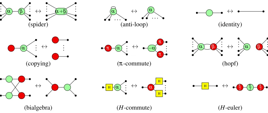
Figure 2: The rules of theZX-calculus. Note all arithmetic is modulo 2π.

J H K=

1

√

2

1 1 1 −1

.

Since the above diagrams are the generators ofZX, the above definition extends uniquely to a strict †-symmetric monoidal functorJ·K:ZX→fdHilb.

The ZX-calculus has a rich equational theory based on the theory of Frobenius-Hopf algebras [7, 10]. Various axiomatisations have been proposed ([12, 13, 5, 23, 16, 22]) with various advantages and drawbacks. Here we adopt the scheme of Backens [3] which is clean, concise, and adequate for the treatment of the Clifford group. These are shown in Figure 2. Note that, due to theH-commute rule, the colour swapped versions of all the rules are admissible, and we shall use these colour swapped versions without further comment.

Definition 3.4. Let↔be the one-step rewrite relation on the terms ofZXgenerated by the pairs of terms shown in Figure 2; let↔∗ be the least equivalence relation containing↔. We say thatZXtermsaandb

areequivalentwhena↔∗ b.

We reserve the notation a=b for the case where a and b are equal as graphs, in the sense of Definition 3.1.

Thanks to theH-euler rule, theHvertices are redundant. With this in mind, the following colour changing rule will be useful.

Lemma 3.5. The following rule is admissible:

α

π/2

π/2

π/2

π/2

π/2

π/2

..

. ...

∗

↔ α+

nπ 2 −π/2

−π/2

−π/2

−π/2

−π/2

−π/2 ..

. ...

where n is the number of red vertices in the left hand side diagram.

4

Representing Clifford Circuits in the

-calculus

For the rest of the paper we will use only thestabilizersub-language of the fullZX-calculus.

Definition 4.1. LetZXsdenote the sub-PROP ofZXobtained by restricting to those terms whoseZand

Xvertices are labelled only by anglesα∈ {0,π/2,π,3π/2}.

Since only four vertex labels can occur in the terms ofZXs, we will adopt a more compact notation as

shown in below.

.. .

+

..

. := .._. π/2 ... ...

π

.. .

+

..

. := .._. π/2 ... .._.

π

Since the one-qubit instances of these will occur very frequently in the rest of the paper, we introduce the names:

+

π

π

x₊: 1→1 x: 1→1 x−: 1→1 z+: 1→1 z: 1→1 z−: 1→1

We refer toxandzas thePaulis.

We define thetranslationfunctorT :Cliff→ZXson the generators as shown below.

T

S

= ₊ T

Z

=

_π

T

V

= ₊ T

X

=

_π

T

H

= H T







 =

This extends to the whole PROP in the usual way. Further we have the following:

Proposition 4.2. For all c:n→m inCliffwe have_Jc_KC=JT(c)K.

Subject to the proviso that the variablesα andβ occurring in the rules of Figure 2 must take values in

the set{0,π/2,π,3π/2}, it is immediate that ifa↔∗ bthenais inZXsif and only ifbis. Further, the

equational theory ofZXsis sound and complete for its standard interpretation.

Theorem 4.3(Backens [3]). Let a and b be terms ofZXs. Then a

∗

↔b if and only if_Ja_K=_Jb_K.

+

π

π

π

π

π

π

π

π

− − + + − + + − − − + + − + +

+

−

− + − + − + + + + +

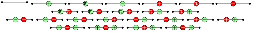
Figure 3:C₁: standard minimal forms for single-qubit Cliffords

4.1 1-Qubit Cliffords

LetC1denote the 24 diagrams shown Figure 3. Note that all of them are in the image of the translation

functorT, so they correspond to Clifford circuits. Further, each of the diagrams has a distinct interpretation underJ·K, so they coverC1and, by soundness, they are not equivalent.

Proposition 4.4. Given t∈Cliff(1,1)then T(t)↔∗ c for some c∈C1.

Proof. From its type, we haveJtKC∈C1and since|C1|=24, necessarilyJtKC=JcKfor somec∈C1, and

thus by Proposition 4.2_JT(t)_K=_Jc_K. From this point the result follows by Theorem 4.3.

Since we will require an effective procedure later, we offer an alternative, constructive, proof which produces the requiredc. The ideas of this proof form an important part of our optimisation procedure.

Recall that aline graphis a framed open graph with one input and one output, which is connected and whose vertices all have degree two. In other words, the graph has the shape of a line. We can treat a line graph as a sequence of vertices starting from the input; let pos(v)denote the sequence position of vertexv, i.e. ifvis the first vertex then pos(v) =0.

Lemma 4.5. Let t∈ZXs(1,1)be a line graph; then t↔∗ s for some s∈ZXs(1,1)which has the following properties:

• its vertices form an alternating sequence of Z(α)and X(β)vertices, where none of the labels are zero;

• it contains at most two Pauli vertices, and if present these are first vertices after the input.

We say that s is inPauli-standardform.

Proof. Observe that by applying theH-euler rule all theHvertices can be removed. Then, by repeated application of the spider and identity rules, we obtain a graph of alternating coloured vertices, none of which are labelled by zero. Now we proceed by induction; define

m(t) =

_∑

pos(v)

Observe that ifm(t)<2 thenthas the required form. Otherwise there is at least one Pauli vertexvwith pos(v)≥2. Suppose thatvis a Pauli Z vertex; then we may rewritet↔∗ t0by the following rewrites:

α β

_π

_π

and applying the identity rule if possible. Note thatZ(α+π)is never a Pauli, so the number of Paulis

Lemma 4.6. We have the following equations:

+ +

+ ↔∗ − − − ↔∗ + + + ↔∗ − − −

− −

+ ↔∗ − + + ↔∗ + − − ↔∗ − + +

+

−

+ ↔∗ − + − ↔∗ + − + ↔∗ − + −

− +

+ ↔∗ − − + ↔∗ + + − ↔∗ − − +

Proof. For the first sequence of equations, consider the following rewrites

+ +

+ →∗ − − − →∗ − −

π

∗

→ −

π

where the first and last steps use Lemma 3.5. The other three cases are established using very similar reasoning.

Alternative proof of Prop 4.4. First observe that for anyt∈Cliff(1,1) its imageT(t) has the form of a line graph. Now, by Lemma 4.5,T(t)↔∗ t1 wheret1 is in Pauli-standard form. Now we proceed by

induction onn, the number of vertices oft₁.

Ifn=0 or 1 thent1is already in C1. If n=2 andt1 has no Pauli nodes, thent1 is already inC1;

otherwiset1 ∗

↔cfor somecinC1by theπ-commute rule.

Ifn=3 andt₁contains at least one Pauli vertex, then by applying theπ commute and spider rules,t1

can rewrite to a term with only two vertices or fewer. For example

α β

π

Otherwise, none of the vertices are Paulis; there are 16 line graphs of this form; by Lemma 4.6 these are partitioned in four equivalence classes. Each of the four equivalence classes contains an element ofC₁, hencet1

∗

↔c∈C₁.

Finally, supposen≥4. Ift1has any Pauli vertices, thent1 ∗

↔t2by (1) wheret2has strictly fewer Pauli

vertices, and strictly fewer vertices overall. Otherwise,t₁has no Pauli vertices; therefore any sequence of vertices of length three can be rewritten, using Lemma 4.6, to a sequence with the colours exchanged. Then by applying the spider and identity rules, and Lemma 4.5t1

∗

→t2wheret2is in Pauli standard form

and has strictly fewer vertices thant₁. Hence we obtain the result by induction.

By enumerating all diagrams with fewer than four vertices, it’s easy to check that noc∈C1is equivalent

to a smaller diagram, so these diagrams are the minimal forms forC1.

4.2 2-Qubit Cliffords

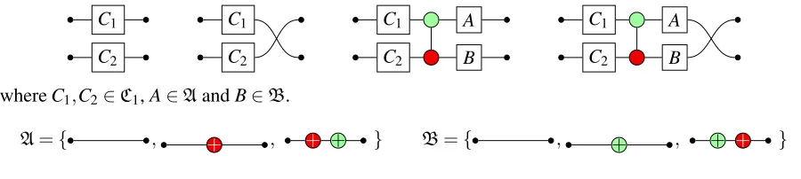
LetC₂be the set of diagrams defined in Figure 4. Notice thatC₂has 242(1+1+9+9) =11520 elements. As in the case ofC₁, all the elements ofC₂are evidently circuits, and it can be mechanically checked that they are all distinct under the standard interpretation. Hence we adoptC2 as the normal forms forC2.

Again, by the completeness of the axioms (Thm 4.3) we can immediately conclude that every 2-qubit Clifford circuit is equivalent to somek∈C₂. Zooming in a little closer we have the following:

Proposition 4.7. Let k∈C2and let g be a generator ofC2 as aZX-calculus term; then g◦k ∗

C1 C2

C1 C2

C1 C2

A

B

C1 C2

A

B

whereC1,C2∈C1,A∈AandB∈B.

A={ , ₊ , + + } B={ , ₊ , + + }

Figure 4:C₂: standard minimal forms for two-qubit Cliffords

Proof. Notice that the 1-qubit CliffordsC1andC2which occur inkplay no part in the computation, hence

we ignore them.

There are effectively four choices forg: (u⊗id), (id⊗u), CNOT, orσ, whereuranges over the generators ofC1. Ifg=σ, the result is trivial.

Further, for anyu∈C₁, we have(u⊗id)◦CNOT= (a⊗id)◦CNOT◦(u₁⊗u₂)for someu₁,u₂∈C₁

anda∈A, either by commuting vertices of the same colour, or taking out factors of Paulis. Similarly

(id⊗u)◦CNOT= (id⊗b)◦CNOT◦(u1⊗u2)for someb∈B. Hence the only non-trival cases to consider

are:

1. g=CNOTandk= (a⊗b)◦CNOT. There are nine possibilities for this case, of which we consider two here. Ifa=x+andb=id, then by using the bialgebra rule we reduce as shown in (i) below. If

a=x+andb=z+, then a similar argument yields (ii).

(i)

+ _∗

↔

++

+

− ++

(ii)

+

+

∗

↔ −

− +

+

+

+

They remaining cases can all be derived from these two, except the case wherea=b=id, which is trivial.

2. g=CNOTandk= (b⊗a)◦σ◦CNOT. In this case we have (iii) below. However, by exploiting the

Hrules we have the equivalence (iv) so this case can be reduced to the previous one.

(iii)

b

a

∗

↔

a

b

(iv) ↔∗

− −

− −

+ +

+ +

3. g=CNOTandk=σ. Again we can apply (iv).

As in the single qubit case these reductions will provide the basis for the rewrite rules of our optimiser.

5

Quantomatic

We briefly sketch the Quantomatic system; for a full description see [18]; to obtain it, see [17].

rulesto the current graph. A rewrite rule is adirectedequation, i.e. a pair of graphs which have the same boundary. Rules are applied in two-step process. First the system searches for subgraphs of the term which are isomorphic to the LHS of the rule; each such subgraph is called amatch. Quantomatic displays all the possible matches of the chosen rule in the current term, and allows the user to select where the rule is to be applied. The matched subgraph is then replaced by the RHS of the rule to produce a new term. A proof therefore consists of a sequence of terms linked by the application of a particular rule at a particular location in the term.

Quantomatic allows the user to define automated proof tactics, known as simplification procedures or

simprocs. The name is slightly misleading since there is no need for a simproc to actuallysimplifythe graph, in the sense of reducing the number of vertices or edges; however failure to do so will typically result in non-termination. Simprocs are written in the Python programming language, interpreted by the built-in Jython interpreter [1], and augmented with various tactic combinators. The most useful of these are:

• REWRITE(r) : given a ruler, apply the rewrite to the first match found.

• REWRITE_METRIC(r,m) : given a rulerand ametricfunctionm:ZX→Napply the rewrite to

the first match found whichreducesthe metric.

• REWRITE_TARGETED(r,v,t) ; given a ruler, a vertexvin the LHS of the rule, and atargeting

functiont:ZX→Vert apply the rewriterto the first match where vertexvof the rule is matched to the vertext(G)in the term.

All of these combinators can also accept a list of rules, in which case the rewrites are attempted in the order of the list. Simprocs can be combined in sequence, and also using the combinator REDUCE(s) which repeats the simprocsuntil no new rewrites can be performed.

An important point is that when multiple matches are obtained, the system will select one without user intervention. Which rewrite is selected depends on the internal representation of the term, and is effectively non-deterministic.

The axioms of theZX-calculus, considered as a rewrite system, are neither terminating nor confluent: for example, ifG→G0via theπ-commute rule then the rule can be applied again immediately to rewrite G0→G. This and similar cases can easily lead to a non-terminating rewrite strategy. Further although many of the axioms can be oriented in a direction which reduces the graph complexity, the resulting rewrite system is no longer complete with respect to the standard interpretation: in some cases it is necessary to increase the graph size to derive a desired equation.

6

Optimising Clifford Circuits with Quantomatic

In this section we describe our optimisation procedure and summarise the results. The reasons for our choices are discussed in the following section.

Bycircuitwe mean aZX-calculus term which is the image of the translation functorT:Cliff→ZX

defined in Section 4. Note that sinceCliffis a†-PROP and_J·_Kis a strict monoidal functor, the circuits form a sub-PROP ofZX: they are closed under composition and tensor product; however they are not closed with respect to the equivalence relation↔∗.

The axioms of theZX-calculus calculus are mostly equations between graphs which are evidently not circuits. Therefore our first step is to derive new equations between circuits which will serve as rewrites for use in the main simproc. These rules are listed in Appendix D.

While the derived rules are “obviously” equations between circuits, the circuit structure of a larger graph may not be apparent by looking at a local subgraph. It’s necessary to look at the entire graph in order to guide the rewrite engine.

Definition 6.1. AZX-calculus diagram is calledsimpleif it satisfies the following criteria:

• It is a simple graph.

• No vertex is adjacent to a vertex of the same colour.

• Every degree 2 vertex has a non-zero label.

Lemma 6.2. EveryZX-calculus diagram is equal to a simple one.

Proof. Starting with an arbitrary diagramd, first replace allHboxes using the H-euler rule. Then apply the spider rule to fuse spiders, the hopf rule to remove parallel edges, the anti-loop rule to remove any self loops, and the identity to remove trivial spiders everywhere.

Definition 6.3. [9] Given a diagramd, with verticesV, inputsI, and outputsO, acausal flow(f,≺)ond

consists of a function f:I+V →V+Oand a partial order≺on the setI+V+Osatisfying the following properties:

(F1) f(v)∼v

(F2) v≺f(v)

(F3) Ifu∼f(v)thenv≺u

wherev∼umeans thatuandvare adjacent in the graph.

In the one-way model [24], the existence of a causal flow on a graph implies that measurement-based quantum computation on the corresponding graph state is deterministic [9]. It plays a similar role for

ZX-diagrams.

Definition 6.4. A simpleZX-diagram is calledcircuit-likeif has the same number of inputs and outputs and its underlying graph admits acausal flow.

Proposition 6.5. Every circuit-like diagram corresponds to a quantum circuit.

Proof. Using the given flow(f,≺)we will translate a circuit-like diagramdinto a circuitcsuch thatcis obvious in the image to ofT.

We must first determine which edges in the diagram correspond to qubits and which correspond to interactions between qubits. Note that for each inputi, the flow function f defines a path through the diagrami→ f(i)→ f(f(i))→ · · ·. By (F2) and the fact that≺is a partial order, such a path must terminate at an output; and by (F3) each such input-to-output path is disjoint. Further, since the numbers of inputs and outputs are the same then every vertex of the diagram must occur on one such path.

Now we translate the vertices into gates tracing along the qubit paths. If the vertex has degree 2 it immediately yields aZα or anXβ gate. If vertexvhas higher degree, let its neighbours, excluding its

immediate predecessor and successor, beu1, . . . ,un. We decomposevintov0,v1, . . .vnas shown below:

α 7→ α v

v0 v1 v2

vn−1 vn · · ·

· · ·

· · · ·

· · ·

vn

vn−1

7→ α

v1 v2

v0

α

v

Note that the new vertices must be compatible with the original ordering, in the sense that ifui∼v∼uj

whereui≺uj then we require thatvi≺vj. By the flow conditions, none of theuibelong to the same qubit

asv, and by the simplicity of the diagram all theuiare the opposite colour tov. Note that the updated

diagram also admits a causal flow, obtained from the original one in the obvious manner. Hence all the higher degree vertices may be decomposed in the same way, to leave the diagram with no vertex of higher degree than three, and non-zero phases only in the degree two vertices. Then all the links between qubits maybe replaced byCNOTgates; since≺defines a partial order on the vertices, we are guaranteed this is well-defined.

Intuitively the flow path cover specifies which edges of theZX-diagram are the “qubits” of the circuit;

those edges not in the path cover define aCNOTacting on two qubits. Assuming that the graph is a circuit, the path cover is relatively easy to compute by starting at each input and finding a successor among its neighbours. If there is ever a choice of successor for a given vertex this choice can be resolved by looking at the other wires. This information is needed frequently by our optimisation procedure. If an unambiguous path cover cannot be constructed then the procedure halts with an error – in this case the input graph was not a circuit.

Our optimiser can be summarised as the repeated alternation of two phases:

• Simplification: apply everywhere possible a strictly reducing set of rules.

• Commutation: using targeting and metric rewrites, apply reversible rules to (i) move Pauli operators closer to the inputs. (ii) move CNOTandTONCgates which act on the same two qubits closed together.

In order to reduce the number of rules, there is an initial phase which replaces all Hadamard,Z(−π

2)and X(−π

2)gates withS,V and Paulis as appropriate. The single qubit gates are then “tidied up” by a final

pass.

The simplification phase is straightforward, exploiting the different cases of 4.7 as the key rules. The commutation phase is more delicate, and makes heavy use of the path cover computation.

For the single-qubit commutation rules we use targeting function which traverses each path starting from the input and applies the rule at the first possible position in the graph. This works very well and, in concert with the simplification rules, is guaranteed to reduce all single qubit Cliffords to one of the forms ofC₁. However this approach fails for rules where a Pauli must commute with aCNOTgate. The

REWRITE_TARGETED method allows the user to identify a single vertex in the rewrite rule with a single vertex in the graph to be matched. However this is rarely sufficient to uniquely determine the overall match. For example, the following rule

π

π

π

can be applied in two different ways to the central diagram below:

π

π

←

π

π

π

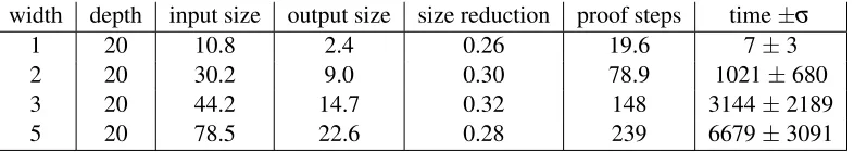
width depth input size output size size reduction proof steps time±σ

1 20 10.8 2.4 0.26 19.6 7±3

2 20 30.2 9.0 0.30 78.9 1021±680

3 20 44.2 14.7 0.32 148 3144±2189

5 20 78.5 22.6 0.28 239 6679±3091

Table 1: Summary of results on randomly generated circuits. Random circuits were generated with the programrandomCliffs.pywhich is available from the project repository. Tests were performed on a basic desktop PC.

necessary information. For this reason, we have defined a metric which favours graphs where the Paulis are nearer to the inputs, and maximally penalises graphs with vertices which are not in any path.

The approach sketched here is very conservative: the optimiser only performs rewrites which result in diagrams which meet the (also very conservative) definition of circuit, even in cases where that diagram could be later rewritten to circuit.

7

Summary of results and discussion

Since we have formalised circuits in theZX-calculus, our measure of size is the number of non-trivial vertices in the graph. This quantity is the gate count over the generating setS,Z,V,X, andCNOT, although

eachCNOTcontributes 2 to the measure. A less obvious consequence of theZX-calculus formalism is that the swap gate is not represented at all, andCNOTgates may act on any qubits without penalty. This may or may not be realistic for a given quantum architecture, but it is a fundamental feature of theZX-calculus,

and removing it would require a string diagrammatic formalism that takes into account the planarity of diagrams. This would take us far beyond the scope of this work.

Our optimiser reduces all one- and two-qubit circuits to elements ofC1andC2respectively; however in

larger circuits it does not always find a minimal form. Notably our ruleset does not include any reductions for circuits of three or more qubits, so there are relatively simpleCNOTcircuits which cannot be reduced. Further, due to the extreme conservativity of our metric and targeting procedures, the optimiser does not always find valid rewrites among the ruleset. However, on a test set of randomly generated Clifford circuits it typically produces significant reductions of circuit size; see Table 1.

There is striking increase in compute time per proof step as the width of the circuit increases. This can be attributed to the increased number ofCNOTgates: as the average vertex degree increases, the number of candidate matches including a given vertex increases geometrically. Since many of these matches will be invalid as circuit rewrites, a lot of time is spent searching for matches which are then rejected. Further, wider circuits require two-qubit commutation rules, which are metric-driven rather than targeted, and hence impose a much greater computational load.

Indeed, the main difficulty we have faced is taking control of the matching engine. Targeted rewriting can select good rewrite positions with high efficiency but does not discriminate between good and bad rewrites at that position. Metric-driven rewrites can perform such discrimination but at the cost of losing control over the search. Combining these features in a single combinator would greatly ease this difficulty.

simprocs.

8

Conclusions and Future Work

Since Quantomatic was designed for interactive use, its simproc environment is currently quite limited. In repurposing the system to operate as a fully automated circuit optimisation tool, we have run up against its current limits, and our frequent resort to brute force and perversity is a reflection of these limitations, rather than the authors’ mental states4. These limitations are not fundamental, and could be removed by minor extensions of the simproc API. Although there is much scope for improvement in our optimiser, we have demonstrated that the Quantomatic system can serve as the basis for an effective circuit optimisation tool.

References

[1] The Jython Project : Python for the Java Platform. Available athttp://www.jython.org.

[2] S. Aaronson & D Gottesman (2004):Improved Simulation of Stabilizer Circuits.Phys. Rev. A70(052328), doi:10.1103/PhysRevA.70.052328.

[3] Miriam Backens (2014): The ZX-calculus is complete for stabilizer quantum mechanics. New Journal of Physics16(9), p. 093021, doi:10.1088/1367-2630/16/9/093021.

[4] Miriam Backens (2015): Making the stabilizer ZX-calculus complete for scalars. In Chris Heunen, Peter Selinger & Jamie Vicary, editors: Proceedings of the 12th International Workshop on Quantum Physics and Logic (QPL 2015),Electronic Proceedings in Theoretical Computer Science195, pp. 17–32, doi:10.4204/EPTCS.195.2.

[5] Miriam Backens, Simon Perdrix & Quanlong Wang (2016):A Simplified Stabilizer ZX-calculus. In R. Duncan & C. Heunen, editors:Proceedings 13th International Conference on Quantum Physics and Logic (QPL 2016),

Electronic Proceedings in Theoretical Computer Science236, pp. 1–20, doi:10.4204/EPTCS.236.1.

[6] Nicholas Chancellor, Aleks Kissinger, Stefan Zohren & Dominic Horsman (2016):Coherent Parity Check Construction for Quantum Error Correction.arXiv.org preprint(arXiv:1611.08012).

[7] Bob Coecke & Ross Duncan (2011):Interacting Quantum Observables: Categorical Algebra and

Diagram-matics.New J. Phys13(043016), doi:10.1088/1367-2630/13/4/043016.

[8] Bob Coecke, Ross Duncan, Aleks Kissinger & Quanlong Wang (2015):Generalised Compositional Theories

and Diagrammatic Reasoning. In G. Chiribella & R. Spekkens, editors:Quantum Theory: Informational

Foundations and Foils, Springer, doi:10.1007/978-94-017-7303-4_10.

[9] V. Danos & E. Kashefi (2006): Determinism in the one-way model. Phys. Rev. A 74(052310), doi:10.1103/PhysRevA.74.052310.

[10] Ross Duncan & Kevin Dunne (2016): Interacting Frobenius Algebras are Hopf. In Martin Grohe, Eric Koskinen & Natarajan Shankar, editors:Proceedings of the 31st Annual ACM/IEEE Symposium on Logic in Computer Science, LICS ’16, New York, NY, USA, July 5-8, 2016, LICS ’16, ACM, pp. 535–544, doi:10.1145/2933575.2934550.

[11] Ross Duncan & Maxime Lucas (2014): Verifying the Steane code with Quantomatic. In Bob Coecke & Matty Hoban, editors:Proceedings 10th International Workshop on Quantum Physics and Logic (QPL 2013),

Electronic Proceedings in Theoretical Computer Science171, pp. 33–49, doi:10.4204/EPTCS.171.4.

[12] Ross Duncan & Simon Perdrix (2009):Graph States and the Necessity of Euler Decomposition. In K. Ambos-Spies, B. Löwe & W. Merkle, editors:Computability in Europe: Mathematical Theory and Computational

Practice (CiE’09),Lecture Notes in Computer Science5635, Springer, pp. 167–177, doi:10.1007/978-3-642-03073-4_18.

[13] Ross Duncan & Simon Perdrix (2014):Pivoting makes the ZX-calculus complete for real stabilizers. In Bob Coecke & Matty Hoban, editors:Proceedings 10th International Workshop on Quantum Physics and Logic, Castelldefels (Barcelona), Spain, 17th to 19th July 2013,Electronic Proceedings in Theoretical Computer Science171, Open Publishing Association, pp. 50–62, doi:10.4204/EPTCS.171.5.

[14] Liam Garvie & Ross Duncan (2018):Verifying the Smallest Interesting Colour Code with Quantomatic. In Bob Coecke & Aleks Kissinger, editors: Proceedings 14th International Conference on Quantum Physics and Logic (QPL 2017), Nijmegen, The Netherlands, 3-7 July 2017,Electronic Proceedings in Theoretical Computer Science266, pp. 147–163, doi:10.4204/EPTCS.266.10.

[15] Daniel Gottesman (1999):The Heisenberg Representation of Quantum Computers. In S. P. Corney, R. Del-bourgo & P. D. Jarvis, editors: Proceedings of the XXII International Colloquium on Group Theoretical Methods in Physics, International Press, pp. 32–43.

[16] Emmanuel Jeandel, Simon Perdrix & Renaud Vilmart (2018):A Complete Axiomatisation of the ZX-Calculus

for Clifford+T Quantum Mechanics. In:LICS ’18- Proceedings of the 33rd Annual ACM/IEEE Symposium

on Logic in Computer Science, arXiv:1705.11151, ACM, doi:10.1145/3209108.3209131.

[17] A. Kissinger, L. Dixon, R. Duncan, B. Frot, A. Merry, D. Quick, M. Soloviev & V. Zamdzhiev:Quantomatic. Available athttp://quantomatic.github.io/.

[18] Aleks Kissinger & Vladimir Zamdzhiev (2015):Quantomatic: A Proof Assistant for Diagrammatic Reasoning. In P. Amy Felty & Aart Middeldorp, editors: Automated Deduction - CADE-25: 25th International Con-ference on Automated Deduction, Berlin, Germany, August 1-7, 2015, Proceedings, Springer, pp. 326–336, doi:10.1007/978-3-319-21401-6_22.

[19] Stephen Lack (2004):Composing PROPs.Theory and Applications of Categories13(9), pp. 147–163.

[20] Saunders Mac Lane (1965):Categorical Algebra.Bull. Amer. Math. Soc.71, pp. 40–106, doi:10.1090/S0002-9904-1965-11234-4.

[21] Dmitri Maslov & Martin Roetteler (2018): Shorter stabilizer circuits via Bruhat decomposition and

quantum circuit transformations. IEEE Transactions on Information Theory 64(7), pp. 4729–4738,

doi:10.1109/TIT.2018.2825602.

[22] Kang Feng Ng & Quanlong Wang (2017):A universal completion of the ZX-calculus. ArXiv:1706.09877.

[23] Simon Perdrix & Quanlong Wang (2016): Supplementarity is Necessary for Quantum Diagram Reason-ing. In Piotr Faliszewski, Anca Muscholl & Rolf Niedermeier, editors: 41st International Symposium on Mathematical Foundations of Computer Science (MFCS 2016),Leibniz International Proceedings in Infor-matics (LIPIcs)58, Schloss Dagstuhl–Leibniz-Zentrum fuer Informatik, Dagstuhl, Germany, pp. 76:1–76:14, doi:10.4230/LIPIcs.MFCS.2016.76.

[24] R. Raussendorf & H. J. Briegel (2001):A One-Way Quantum Computer.Phys. Rev. Lett.86, pp. 5188–5191, doi:10.1103/PhysRevLett.86.5188.

A

Electronic Resources

All the work described in this paper is available as a downloadable quantomatic project from the following URL.

https://gitlab.cis.strath.ac.uk/kwb13215/Clifford-Quanto/

Please download it and play around!

B

An aside on CNOT and SWAP

We have already seen theZX-calculus representation ofCNOTin Section 4. Note that the upper (z) vertex corresponds to the control qubit, while the lower (x) is the target qubit. We could also consider theCNOT

with control and target reversed, which we denoteTONC.

TONC := =

It is a well known fact that the swap itself can be represented asCNOT◦TONC◦CNOT, and indeed this is provable in theZX-calculus.

∗

↔ ↔∗ ↔∗ ↔∗ (2)

Note that the bialgebra rule gives the first equation, and the Hopf rule the second: we cannot rely purely on the group structure.

Alternatively, by the colour duality principle we can expressTONCin terms ofCNOTandH:

∗

↔

H

H H

H

∗

↔

− −

− −

+ +

+ +

(3)

Combining (3) and (2) we obtain:

Lemma B.1.

∗

↔

π

π

−

−

+

+ +

+ +

+

Lemma B.1 indicates that we can dispense with the swap as well asTONCand work purely withCNOT. Since we have formalised the system as a PROP it is more convenient to treatσ as one of the generators

C

Proofs omitted from main article

α π/2 π/2 π/2 π/2 π/2 π/2 .. . ... ∗

↔ α+

nπ 2 −π/2

−π/2

−π/2

−π/2

−π/2

−π/2

..

. ...

wherenis the number of red vertices in the left hand side diagram.

Proof. Consider a single red spider. By the H-rules, and the spider we may reason as follows:

α .. . ... ∗ → α .. . ... ∗ → α .. . ... ∗ → α .. . ... + + + + + + + + + + + + + + + + + + ∗

→ α+nπ/2

.. . ... + + + + + + + + + + + +

From which the result follows by applyingz−to every leg.

Proposition 4.7 Letk∈C₂and letgbe a generator of C2as aZX-calculus term; theng◦k ∗

↔k0 for somek0∈C₂.

Here we fill in the missing details behind the equations (i) – (iv) that appeared in the proof.

Equation (i): + _∗ ↔ ++ + − ++ Proof. + ∗ ↔ + ∗ ↔ ₊ ↔∗ +− − + − + + ∗ ↔ ++− + + + + + ∗ ↔ ++− + + + − + + + ∗ ↔ ++− −

π

π

Equation (ii): + + ∗ ↔ − − + + + + Proof. + + ∗ ↔

π

π

π

π

π

π

π

π

π

π

π

π

π

π

π

Note that we have used both Equations (2) and (3) in the heart of this proof.

Equation (iii): b a ∗ ↔ a b

Proof. This is a straightforward application of the “topology” principle; no rules are required, they are equal in the sense of Definition 3.1.

Equation (iv): ∗ ↔ − − − − + + + +

D

Main Rules

The following derived rules are the core of the circuit transformations in the main proof development. The rules themselves are found inderived-rules/in the Quantomatic project, and their derivations are found inderived-rules-proofs/.

In all diagrams inputs are to the left, outputs to the right.

D.1 Init

These rules remove all minus and H nodes from the graph.

− →

π

− →

π

H → + + +

D.2 Always Rules

These are strictly reducing so can always be applied.

π π

π

π

π

π

+ + →

π

π π

π

π

π

π

+ +

+ + →

π

+ + →

π

→

+ +

→

+

π

+

+

+

+ +

+ + → ₊

+

+ +

+

→ +

+ +

+ +

π

+

+

→ +

+ + + +

π

+

+ +

→

+

π

+

+ +

+ +

π

D.3 EulerProc

+ + + → + + +

The inverse is also used.

D.4 Pauli Commutation rules

Each of these is managed by a custom simproc which searches for a good place to apply them.

+

π

π

π

π

+ →

π

π

π

x →

π

π

These rules are used by the Pauli Commutation proc, which is based on REDUCE_METRIC.

x

→ x

π

π

π

π

→

π

π

x → x

D.4.1 C2 Rules

These two alternate in the C2Proc simproc. Both have a custom targeting routine to select where they should be applied.

x _→ x