Dimensionality Reduction Based on Determinantal Point Process and Singular
Spectrum Analysis for Hyperspectral Images
Weizhao Chen
1, Zhijing Yang
1*, Faxian Cao
1, Yijun Yan
2, Meilin Wang
1, Chunmei Qing
3,
Yongqiang Cheng
41 School of Information Engineering, Guangdong University of Technology, Guangzhou, 510006, China 2 Department of Electronic and Electrical Engineering, University of Strathclyde, Glasgow, UK
3 School of Electronic and Information Engineering, South China University of Technology, Guangzhou, China 4 School of Engineering and Computer Science, University of Hull, Hull, HU6 7RX, UK
Abstract: Dimensionality reduction is of high importance in hyperspectral data processing, which can effectively reduce the data redundancy and computation time for improved classification accuracy. Band selection and feature extraction methods are two widely used dimensionality reduction techniques. By integrating the advantages of the band selection and feature extraction, we propose a new method for reducing the dimension of hyperspectral image data. First, a new and fast band selection algorithm is proposed for hyperspectral images based on an improved Determinantal point process (DPP). To reduce the amount of calculation, the Dual-DPP is used for fast sampling representative pixels, followed by kNN-based local processing to explore more spatial information. These representative pixel points are used to construct multiple adjacency matrices to describe correlation between bands based on mutual information. To further improve the classification accuracy, two-Dimensional Singular Spectrum Analysis (2D-SSA) is used for feature extraction from the selected bands. Experiments show that the proposed method can select a low-redundancy and representative band subset, where both data dimension and computation time can be reduced. Furthermore, it also shows that the proposed dimensionality reduction algorithm outperforms a number of state-of-the-art methods in terms of classification accuracy.
1. Introduction
Unlike traditional two-dimensional (2-D) images, hyperspectral data contains a 3-D structure, i.e. 2-D spatial information and 1-D spectral information. Abundant spectral information can describe the ground targets in more detail.
Such advantages have facilitated the fast development of hyperspectral images in the field of remote sensing [1-2], where it has been successfully applied in urban mapping, environmental management, crop analysis, and mineral detection [3]. In addition to remote sensing, hyperspectral images has also been applied in lab-based applications such as forensics, pharmaceutical, medical, and food quality analysis [4-7].
Although more spectral bands can increase the representation of ground objects, not all the bands play equally important roles in hyperspectral data processing [8]. Excessive data dimensions will directly lead to increased computational complexity and computer memory resources. In addition, high dimensional dataset may cause the Hughes phenomenon, which will lead to a decline in classification accuracy [3].
To solve these problems, dimensionality reduction for hyperspectral images has attracted great attention in the past decade. Relevant techniques can be mainly divided into two categories, i.e. band selection and feature extraction.
Band selection can also be regarded as a feature selection process [9-14], which aims to select a subset of the spectral features from the original data whilst keep the dominant information and maintain the performance. In [15], Yao et al proposed a new filter-based feature extraction method for band selection. The advantage of band selection
is that it retains the physical information, characteristics and interpretable ability of the original data [9]. According to whether the sample labels are known or not, the band selection methods for hyperspectral images can be classified into supervised band selection [16-17] and unsupervised band selection [18-20].
Under the condition that a part of the sample labels is known, the supervised band selection method can select bands with higher correlation with class labels. In [12], the correlation between features and class labels is considered in designing a mutual-information based band selection algorithm. In comparison to unsupervised band selection methods, supervised band selection in general has better performance [21]. However, unsupervised band selection is still needed especially when there is no (sufficient) labelled data for supervised learning, regardless the time-consuming process of data labelling.
For most unsupervised band selection algorithms, they aim to preserve the information of the original data with lowest possible dimensional dataset. Therefore, the generic unsupervised band selection algorithm contains two steps. The first is to establish an effective criterion to evaluate the spectral band performance or the redundancy of the candidate band subset. The second is to find a search strategy to determine a suitable band subset.
2
categorized into local-based methods and global-based methods.
Local-based methods map the data from high dimension to low dimension whilst maintaining the local structure. Examples include Locality Preserving Projection (LPP) [26] and Locally Linear Embedding (LLE) [27]. In [28], Guo et al proposed a novel sparse hashing method to embed the high-dimension features into a low-dimension Hamming space.
The global-based approaches aim to obtain a low dimensional representation of the original data whilst maintain the global structure of the original data. Typical examples include Principal Component Analysis (PCA) [29] and Isometric Feature Mapping (ISOMAP) [30]. In addition, some feature extraction methods can greatly remove the image noise, such as two-dimensional empirical mode decomposition (2D-EMD) [31] and two-dimensional singular spectrum analysis (2D-SSA) [22]. 2D-EMD can reconstruct each image using extracted low-order IMFs which can present the spatial structure of the image. 2D-SSA can decompose each image into varying trends, oscillations, and noise. The image can be reconstructed using the trend and selected oscillations whilst remove the noise. In general, feature extraction methods can achieve high accuracy in classification of hyperspectral images.
In summary, band selection and feature extraction methods have their own advantages and disadvantages for dimensionality reduction. Band selection methods can effectively maintain the original spectral band information and the correlation between spectral bands. Besides, band selection can directly remove the redundant information from the hyperspectral datasets. However, band selection normally is difficult to greatly improve the classification accuracy. On the contrary, feature extraction can effectively use the potential features of the hyperspectral image and achieve higher classification accuracy. However, feature extraction is usually applied to the original hyperspectral images and does not take into account the redundancy of the spectral bands.This will also result in the redundancy after feature extraction. Moreover, it will take more computation time for feature extraction because of the redundant information. In order to solve these problems, we combine band selection and feature extraction and propose a new dimension reduction method for hyperspectral image as detailed below.
First, we designed a fast band selection method using the spatial information. In [8], Yuan et al proposed a multiple graph to describe the complex structure between spectral bands by using spectral clustering. This method can consider latent structure between spectral bands in the high dimensional space thus it helps to make full use of the spatial information for more comprehensive measurement of the spectral redundancy. However, constructing a multiple graph structure by spectral clustering requires extremely high computation time and memory. To tackle this problem, we sample representative pixels to measure the correlation between bands. This sampling method consists of two steps: we first use Dual Determinantal Point Process (Dual-DPP) [32] to fast sample representative pixels, followed by kNN based strategy to determine neighbouring pixels to supplement the number of samples.
Afterwards, we use the mutual information to construct an adjacency matrix that can describe the
correlation of the spectral bands with representative pixels in each group. In this way, we can obtain multiple adjacency matrices from representative pixels in different groups. These adjacency matrices can measure redundancy of spectral bands using different spatial information. In addition, we also improved the original k-Determinantal point process (k-DPP) [33] to enable it to select a diversity and low-redundancy band subset from different adjacency matrices. Finally, to improve the classification accuracy, we use 2D-SSA to extract the spatial features from a low-redundancy and low-dimension band subset.
The main contributions of this paper can be summarized as follows:
1. A fast Dual-DPP and kNN based algorithm is proposed to sample sufficient representative pixels from each spectral band.
2. From the perspective of data distribution, spatial information from different regions is used to measure the redundancy of the spectral bands more comprehensively. Moreover, we have improved the original k-DPP algorithm so that it can select low-redundancy spectral band subsets on multiple similarity matrices.
3. We apply 2D-SSA to selected subset of bands to better extract spatial features to improve the classification accuracy under much lower feature dimensions whilst effectively reducing the computational time.
2. Related background
2.1 k-Determinantal Point Process
Determinantal point process (DPP) is an elegant probabilistic model of repulsion that arises in quantum physics and random matrix theory [32]. DPP is an effective and accurate sampling method, which can select a diversity and low-redundancy subset. DPP has many applications in real-world such as summarization, image search and news threading [32]. First proposed by Macchi [34], the DPP cannot set the cardinality 𝑘 of the subset bands in advance. To solve this problem, Kulesza et al [33] proposed an improved DPP algorithm called k-DPP to model the sets of cardinality 𝑘 as follows.
Given a discrete finite set γ = {1,2,3, … , N}, any candidate subset 𝑌 ⊆ γ with cardinality |𝑌| = 𝑘 is selected according to the probability
𝑃𝐿𝑘(𝑌) =∑ det(Ldet(L𝑌)
𝑌′)
|𝑌′|=𝑘 (1)
where 𝑌′ represents all the subsets that their cardinality, |𝑌′|, is equal to 𝑘. L𝑌 is a symmetric positive semidefinite matrix and its entries are indexed by the corresponding elements of 𝑌. Similarly, L𝑌′ is a symmetric positive semidefinite matrix whose entries are indexed by the corresponding elements of 𝑌′. Each element of matrix L
𝑌 represents the correlation of the corresponding two elements in 𝑌.
For example, if the subset 𝑌 contains two elements
𝑌 = {𝑖, 𝑗}, L𝑌 can be written as
L𝑌= [
𝐿𝑖𝑖 𝐿𝑖𝑗
3
The greater the correlation between elements 𝑖 and 𝑗 will result in the larger value of 𝐿𝑖𝑗 and 𝐿𝑗𝑖.Then the probability of selectingcandidate subset 𝑌 can be expressed as follows:
𝑃𝐿𝑘(𝑌) ∝ det(𝐿𝑌)
∝ |𝐿𝐿𝑖𝑖 𝐿𝑖𝑗
𝑗𝑖 𝐿𝑗𝑗| (3)
Obviously,the larger values of 𝐿𝑖𝑖 and 𝐿𝑗𝑗mean that the elements 𝑖 and 𝑗 are more likely to belong to the subset 𝑌. The large value of 𝐿𝑖𝑗 means that 𝑖 and𝑗 seem unlikely to co-occur. The more diverse and lower-redundancy subset has larger 𝑃𝐿𝑘(𝑌).
However, selecting 𝑌 from γ according to the equation (1) is an NP-hard problem. In [33], an approximate solution is given. The k-DPP mainly contains two steps [33]. In the first step, the eigenvector subset 𝑉 with 𝑘 eigenvectors are selected depending on the probability which is calculated by the corresponding eigenvalues. In the second step, we select the band subset according to eigenvectors in subset 𝑉.
An example is given below to
detail the selection process.Given a positive semidefinite matrix 𝐿, its entries are indexed by the corresponding elements of γ. 𝐿 can be decomposed as
𝐿 = ∑𝑁𝑛=1𝜆𝑛𝜈𝑛𝜈𝑛𝑇 (4)
𝜆𝑛 is the eigenvalue of 𝐿 and 𝜈𝑛 is the corresponding eigenvector. Then we want to find a subset 𝑌 from γ whose cardinality is |𝑌| = 𝑘. First, we select 𝑘 eigenvalues 𝑆 =
{𝜆1, 𝜆2, … , 𝜆𝑘−1, 𝜆𝑘} and the corresponding eigenvectors
𝑉 = {𝜈1, 𝜈1, … , 𝜈𝑘−1, 𝜈𝑘}. Define 𝑆′⋃𝜆𝑘= 𝑆, then the cardinality |𝑆′| = 𝑘 − 1. The probability of selecting the k -th eigenvalue, 𝜆𝑘, corresponding to the eigenvectors 𝜈𝑘 of 𝐿 to add to 𝑆 and 𝑉 can be expressed as:
P(𝜆𝑘∈ 𝑆) = 𝜆𝑛𝑒𝑘−1
𝑛−1
𝑒𝑘𝑛 (5)
where 𝑒𝑘𝑛= ∑|𝑌|=𝑘∏𝑛∈𝑌𝜆𝑛. In the second step, denote the low-redundancy band subset as 𝑌, whose cardinality is k, that is, |𝑌| = 𝑘 and 𝑌′∪ 𝑖 = 𝑌. The probability of selecting the 𝑖-th band to add to𝑌 can be written as:
𝑃𝑟(𝑖) =|𝑉|1∑𝜈𝑛∈𝑉(𝜈𝑛𝑇𝑒𝑖)2 (6)
where 𝑒𝑖 is a column vector that the 𝑖 element is one and the other elements are zero.
2.2 2D-Singular Spectrum Analysis
The 2D-SSA can extract the trend and select oscillations from hyperspectral images as features and remove the noise [22]. It contains four steps:Embedding 2-D Signal, SV2-D, Grouping, and 2-Diagonal Averaging.
Embedding 2-D Signal: we set each spectral image
𝑃2𝐷 with a size 𝑛
𝑥× 𝑛𝑦. Each spectral image can be represented as a matrix:
P2D=
[
p1,1 p1,2 ⋯ p1,ny
p2,1 p2,2 ⋯ p2,ny
⋮ ⋮ ⋱ ⋮
pnx,1 pnx,2 ⋯ pnx,ny]
(7)
𝑃2𝐷 can be written as a trajectory matrix 𝑋2𝐷 with Hankel-block-Hankel structure:
𝑋2𝐷=
[
𝐻1 𝐻2 ⋯ 𝐻𝑁𝑥−𝐿𝑥+1
𝐻2 𝐻3 ⋯ 𝐻𝑁𝑥−𝐿𝑥+2
⋮ ⋮ ⋱ ⋮
𝐻𝐿𝑥 𝐻𝐿𝑥+1 ⋯ 𝐻𝑁𝑥 ]𝐿𝑥×(𝑛𝑥−𝐿𝑥+1)
(8)
where each submatrix 𝐻𝑟 is Hankel type defined by
𝐻𝑟=
[
𝑝𝑟,1 𝑝𝑟,2 ⋯ 𝑝𝑟,𝑛𝑦−𝐿𝑦+1
𝑝𝑟,2 𝑝𝑟,3 ⋯ 𝑝𝑟,𝑛𝑦−𝐿𝑦+2
⋮ ⋮ ⋱ ⋮
𝑝𝑟,𝐿𝑦 𝑝𝑟,𝐿𝑦+1 ⋯ 𝑝𝑟,𝑛𝑦 ]𝐿
𝑦×(𝑛𝑦−𝐿𝑦+1)
(9)
where 𝐿𝑥 and 𝐿𝑦 are the sizes of 2D-windows.
SVD: Matrix 𝑆 is defined by the trajectory matrix 𝑋2𝐷 as follows:
𝑆=𝑋2𝐷𝑋2𝐷𝑇 (10)
The eigenvalues of 𝑆 are denoted as {𝜆1≥ 𝜆1≥ ⋯ 𝜆𝐿} and the corresponding eigenvectors are {𝜇1, 𝜇2, … , 𝜇𝐿}, where 𝐿 = 𝐿𝑥× 𝐿𝑦.
Grouping
:
The total set of
L components is divided into two disjoint sets according to their contribution. The contribution of each component is related to its eigenvalue which can be represented as𝜂𝑡=∑∑𝑙∈𝑡𝐿 𝜆𝑙𝜆𝑙
𝑙=1 (11)
𝑡 is the set of eigenvalues with large values. Then we select the set with higher 𝜂𝑡 to reconstruct the matrix 𝑋𝑡𝑀2𝐷.
Diagonal Averaging: This process contains two-step Hankelization process. Sequential Hankelization is first applied within each block 𝐻𝑟 and then applied between the blocks 𝑋2𝐷. Then 2D diagonal projection from group 𝑋𝑡𝑀2𝐷 can be written as follows
𝑍𝑀2𝐷=
[
𝑧𝑚1,1 𝑧𝑚1,2 ⋯ 𝑧𝑚1,𝑛𝑦
𝑧𝑚2,1 𝑧𝑚2,2 ⋯ 𝑧𝑚2,𝑛𝑦
⋮ ⋮ ⋱ ⋮
𝑧𝑚𝑛𝑥,1 𝑧𝑚𝑛𝑥,2 ⋯ 𝑧𝑚𝑛𝑥,𝑛𝑦]
(12)
Finally, the spectral image 𝑃2𝐷 can be described as
𝑃2𝐷= 𝑍
12𝐷+ 𝑍22𝐷+ ⋯ + 𝑍𝑀2𝐷= ∑𝑀𝑚=1𝑍𝑚2𝐷 (13)
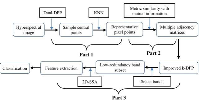
3. The proposed band selection framework
4 Hyperspectral
image
Sample central points Dual-DPP
Representative pixel points KNN
Multiple adjacency matrices Metric similarity with
mutual information
Low-redundancy band
subset Improved k-DPP
Select bands Feature extraction
2D-SSA Classification
Fig.1. The flowchart of the proposed dimensionality reduction method Part 2
Part 3 Part 1
The proposed approach consists of three parts. In Part 1, a fast yet effective sampling algorithm based on Dual-DPP and kNN is introduced to sample the most representative pixels from the spectral datasets. In Part 2, these representative pixels are used to construct multiple adjacency matrices to describe the relationships of band pairs measured by the mutual information. In Part 3, an improved k-DPP algorithm is presented to select a low-redundancy subset of bands from multiple adjacencies. In addition, 2D-SSA is employed to extract the spatial features from the selected bands to further improve the classification accuracy. Details will be discussed in the following subsections.
In section 3.1, we introduce the proposed method to fast sample representative pixel points from hyperspectral images. The method of constructing multiple adjacency matrices is proposed in section 3.2. In section 3.3, we introduce the process of selecting bands with the proposed method and use 2D-SSA to extract spatial feature from the selected band subset.
3.1 Sample representative pixels
A hyperspectral image can be written asB =
{b1, b2, b3, … , b𝑙} ∈ Rn×𝑙, wheren represents the number of pixels in each spectral band and 𝑙 is the total number of spectral bands. b𝑖(1 ≤ 𝑖 ≤ 𝑙) is the 𝑖-th spectral band. We use 𝑝𝑖𝑥 to represent the pixel points in 𝑖-th spectral band.
In this section, we aim to select some representative pixel points from the hyperspectral spatial-domain for subsequent band selection. These pixel points must be diverse and widely distributed in the spatial domain. The algorithm k-DPP mentioned above can be applied for this purpose. However, the k-DPP inevitably needs to compute
𝐿 = 𝐵𝐵𝑇∈ 𝑅𝑛×𝑛 and perform the eigen-decomposition on
𝐿.As shown in equation (4), if the dimension 𝑛 of 𝐿 is large, it will require a huge amount of computer memory and a huge amount of computation time. Therefore, it is impractical to apply this method directly.
To tackle this problem, the Dual-DPP [32] is applied here for fast sampling tasks. Different from 𝐿 = 𝐵𝐵𝑇∈ 𝑅𝑛×𝑛, we construct another adjacency matrix 𝐻 = 𝐵𝑇𝐵 ∈
𝑅𝑙×𝑙, where 𝑙 is the number of bands and 𝑛 is the number of pixels. Since 𝑙 is much smaller than 𝑛, it’s obvious that the dimension of 𝐻 is much smaller than the dimension of 𝐿. Therefore, Dual-DPP requires less memory and less time than k-DPP in the decomposition process. 𝐻 can be decomposed as
𝐻 = ∑𝑙𝑛=1𝜆̂𝑛𝜈̂𝑛𝜈̂𝑛𝑇 (14)
where 𝜆̂𝑛 is eigenvalue of 𝐻 and 𝜈̂𝑛 is the corresponding eigenvector.It can be simply proved that
𝜈𝑛= 𝐵𝑇𝜈̂𝑛 (15)
Therefore, the sampling process by the Dual-DPP method also includes two steps.The first step is the same as the k-DPP method. According to equation (5), eigenvalues subset 𝑉̂ with 𝑘̂ eigenvalues 𝜈̂𝑛 are selected. In the second step, different from equation (6), we select i-th bands by the following probability
𝑃𝑟(𝑖) =|𝑉̂|1∑𝜈̂𝑛∈𝑉̂((𝐵𝑇𝜈̂𝑛)𝑇𝑒𝑖)2 (16)
We repeat the selection process for multiple times until the required number 𝑘̂ (0 < 𝑘̂ ≤ 𝑙) is met.
Due to the dimensionality limit of matrix 𝐻, the value of 𝑘̂ is normally smaller than 𝑙. It will inevitably lead to insufficient samples. In order to solve this problem, we use KNN [35] to increase the number of pixel points.
First, the pixel points collected by Dual-DPP [32] are used as the central points, which can be recorded as a central point set 𝑃𝑐= {𝑃𝑐1, 𝑃𝑐2… , 𝑃𝑐𝑘̂} ∈ ℛ𝑙×𝑘̂, where 𝑙 is the number of bands and 𝑘̂ is the number of central points.
[image:4.595.136.457.136.298.2]5
3.2 Construct multiple adjacency matrices with mutual information
Graph model can effectively capture the relationship between vertices. In [8], the author proposed a multi-graph structure by spectral clustering method that can effectively represent the relationship between bands. However, the spectral clustering methods are too complicated and require lots of computer memory.
To tackle this problem, considering the useful information in spatial domain, we use representative pixels to construct multiple adjacency matrices with mutual information metrics. With this model, we can consider the redundancy of spectral bands from the data distribution of each band and capture the complex relationships between the pairwise bands. Both aspects make our model more comprehensive in judging the redundancy between spectral bands.
We use a fast algorithm [36] to estimate the mutual information between two bands. Assume that pixels (𝑝𝑖,α𝑥, 𝑝𝑗,α𝑥 ), 𝑥 = 1, … , 𝑚, in the α-th cluster from any pairwise bands 𝑏̂𝑖 and 𝑏̂𝑗, and the joint probability of pixel points in α-th cluster from any pairwise bands 𝑏̂𝑖 and 𝑏̂𝑗 can be estimated as
𝑓(𝑝𝑖,𝛼, 𝑝𝑗,𝛼)
=1
𝑚∑
1 2𝜋ℎ2𝑒
−2ℏ12((𝑝𝑖,𝛼−𝑝𝑖,𝛼𝑥)2+(𝑝𝑗,𝛼−𝑝𝑗,𝛼𝑥)2) 𝑚
𝑥=1
(17)
The marginal probability of pixels in the α-th cluster from any band 𝑏̂𝑖 can be estimated by
𝑓(𝑝𝑖,𝛼) = 1
𝑚∑
1 √2𝜋ℎ2𝑒
−1
2ℏ2((𝑝𝑖,𝛼−𝑝𝑖,𝛼𝑥)2 𝑚
𝑥=1
(18)
Combining equations (17) and (18), we can get the mutual information of α-th cluster from any pairwise bands 𝑏̂𝑖 and 𝑏̂𝑗 as
I(b̂𝑖,α, b̂𝑗,α)
=1
𝑚∑ 𝑙𝑜𝑔
𝒎 ∑ ⅇ−𝟐ℏ𝟏𝟐((𝒑𝒊,α𝒙 −𝒑𝒊,α𝒚 ) 𝟐
+(𝒑𝒋,α𝒙 −𝒑𝒋,α𝒚 ) 𝟐
) 𝒎
𝒚=𝟏
∑ ⅇ−𝟐ℏ𝟏𝟐((𝒑𝒊,α𝒙−𝒑𝒊,α𝒚) 𝟐 𝒎
𝒚=𝟏 ∑ ⅇ
−𝟏
𝟐ℏ𝟐((𝒑𝒋,α𝒙−𝒑𝒋,α𝒚) 𝟐 𝒎
𝒚=𝟏 𝑚
𝑥=1
(19)
where I(b̂𝑖,α, b̂𝑗,α) indicates the mutual information between 𝑖-th and 𝑗-th bands calculated by the pixel points of α-th cluster. According to equation (19), we can calculate the mutual information between all bands and construct adjacency matrices LαMI.Through the above method, we can
build multiple adjacency matrices 𝐿𝑀𝐼=
{L1MI, L2MI,L3MI, … , LαMI}(1 ≤ α ≤ k̂), where LαMI∈ 𝑅𝑙×𝑙 is a symmetric matrix used to measure the correlation between spectral bands with pixel information from the α-th cluster.
3.3 Band selection and feature extraction
Taking into account the spatial information of the hyperspectral image, we have construct multiple adjacency matrices with mutual information mentioned in Section 3.2.
In this section, we propose an improved k-DPP to sample low-redundancy set of bands from these multiple adjacency matrices. According to Ref. [8], our algorithm can be written as follows:
𝑃𝐿𝑘𝑀𝐼(𝑌) =
1 𝑘̂∑
1 𝑒𝛼,𝑘𝑁 ∑ 𝑃
𝑉𝑌𝐵
|𝑌|=𝑘 (𝑌′) ∏𝑛∈𝑌𝜆𝛼𝑛 𝑘̂
𝛼=1 (20)
where 𝑒𝛼,𝑘𝑁 = ∑|𝑌|=𝑘∏𝑛∈𝑌𝜆𝛼𝑛 are the eigenvalue polynomials of adjacency matrices 𝐿𝑀𝐼, and 𝑃𝐿𝑀𝐼𝑘 (𝑌) is the probability of sampling a band subset 𝑌 from the all band set γ. 𝜆𝛼𝑛 is eigenvalue of LαMI and ν𝑛𝛼 is corresponding eigenvector. The probability of selecting 𝑖 -th band to add to𝑌 can be written as:
𝑃𝑟(𝑖) =
1 k̂∑
1
|𝑉𝛼| ∑ (ν𝑛𝛼𝑇𝑒𝑖) 2
ν𝑛𝛼∈𝑉𝛼
k̂
𝛼=1
(21)
Our algorithm consists of two steps. The first step is to select the 𝑘 feature vectors in the same way as stated in Section 2.1. The main difference is that we have to select different feature vectors on different adjacent matrixes. In the second step, we select 𝑘 bands, according to the probability calculated in equation (21).Finally, we input the selected spectral band subset into the 2D-SSA algorithm for feature extraction. Details of the final proposed method are summarized in Algorithm 1.
4. Experimental result
In this section, we use two well-known hyperspectral image datasets to test the performance of the proposed method. Several representative unsupervised dimensionality reduction algorithms are used for comparisons, including PCA [29], LPP [26] and EMAP [37]. All the experiments were performed on Matlab and run on Intel CPU [email protected] with 32GB RAM.
4.1. Hyperspectral Datasets
AVRIS sensor: Indian Pines dataset
T
he India Pines dataset was obtained by the Airborne Visible/Infrared Imaging Spectrometer sensor (AVIRIS) in 1992 [38]. The image covers Indian Pines test site in North-western Indiana. It has 220 spectral bands covering the spectrum range of 0.2-2.4 𝜇𝑚. And 20 water absorption spectral bands [104-108], [150-163] are removed and remaining 200 spectral bands form the dataset. It has145 × 145 spatial pixels, including 16 classes ground truth.
ROSIS sensor: Pavia University dataset
6
Algorithm 1 Dimensionality reduction based on DPP and SSA
Input:
𝐵: a hyperspectral image 𝑘: number of selected bands Output:
Y∗: The feature map of B
1) Sample representative pixel points by Dual-DPP and kNN
2) for pixel points of each cluster do
calculate multiple adjacency matrices LαMI by equations (19)
3) end for
4) for each adjacency matrices LαMIdo
5) Characteristic decomposition: {ν𝑛𝛼, 𝜆𝛼𝑛}𝑛=1𝑙 ⇐ LαMI
6) Select 𝑘 eigenvectorswith probability 𝜆𝛼 𝑒𝑛 𝐵,𝑘−1 𝑛−1
𝑒𝐵,𝑘𝑛
7) end for
8) Select band subset Y with equations (21) 9) Extract spatial features Y∗from Y
Output:Y∗
4.2. Experimental parameter setup
[image:6.595.312.499.237.370.2]In this section, we will introduce the parameter settings.We collected 20 pixel points as central points, and each central point selects the closest 50 and 30 pixel points in Indian Pines image and Pavia University image, respectively. The parameter, h, i.e. the width of the kernel in equation (18), is set to be 0.00032 and 0.0024 in Indian Pines image and Pavia University image, respectively. We use the SVM algorithm [40] to test the performance of the selected bands.
The parameters C and RBF kernel of SVM
are determined by five-fold cross validation. In all experiments, 5% of the samples are randomly selected for training, and the rest of the data are used for testing and all experiments are repeated 10 times. The number of training samples and test samples for Indian Pines image and Pavia University imageare shown inTables 1 and 2,respectively. The results of the experiment are evaluated with three authoritative indexes: overall accuracy (OA), average accuracy (AA) and kappa coefficient [41].Table 1 The numbers of training and test samples of each class in the Indian Pines image
Class Training Test Samples
1. Alfalfa 3 51 54
2. Corn-notill 72 1362 1434 3. Corn- mintill 42 792 834
4. Corn 12 222 234
5. Grass- pasture 25 472 497 6. Grass-trees 37 710 747 7. Grass-pas- turemowed 2 24 26 8. Hay- windrowed 24 465 489
9. Oats 2 18 20
10. Soybean- notill
48
920 96811. Soybean- mintill 123 2345 2468
12. Soybean- clean 31 583 614
13. Wheat 11 201 212
14. Woods 65 1229 1294 15. Building- grass-trees 19 361 380 16. Stone- steel-towers 5 90 95
total 521 9845 10366
Table 2 The numbers of training and test samples of each class in Pavia university image
Class Training Test Samples
1. Asphalt 332 6299 6631 2. Meadows 933 17716 18649 3. Gravel 105 1994 2099 4. Trees 153 2911 3064 5. Painted metal sheets 67 1278 1345 6. Bare soil 252 4777 5029 7. Bitumen 67 1263 1330 8. Self-blocking bricks 184 3498 3682 9. Shadows 48 899 947
Total 2141 40635 42776
4.3. Classification performance
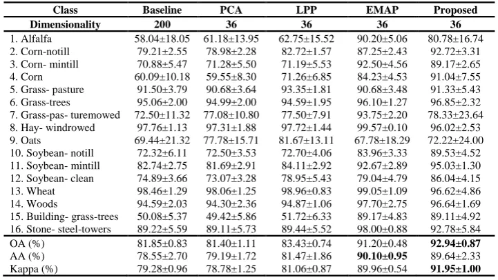
In this section, we choose different dimensionality reduction methods to reduce the dimension of the data and compare the performance of the reduced dimension data on the classification task. All experiments are repeated 10 times, and the relevant mean and standard of classification accuracy deviation are shown in Table 3 and Table 4, respectively.
From Table 3, it can be seen that except the PCA algorithm, the classification accuracies of the other three data dimensionality reduction methods are all higher than that of the original data in Indian Pines dataset. Compared to the original dataset, our algorithm has 11% increase in the indexes of OA and AA, and 12% increase in the indexes of Kappa. Compared to EMAP, our algorithm has 1.7-2% increase in the indexes of OA and Kappa, and 0.3% slightly lower in the indexes of AA. Our method can achieve good results, mainly because our algorithm can effectively select a wide distribution of light bands, which can effectively maintain the original data information. Moreover, our algorithm can effectively extract spatial feature information.
[image:6.595.98.286.551.693.2]7
Table 3 Classification accuracy in the Indian Pines with PCA, LPP, EMAP and the proposed method (Best result of each row is marked in bold type)
Class Baseline PCA LPP EMAP Proposed
Dimensionality 200 36 36 36 36
1. Alfalfa 58.04±18.05 61.18±13.95 62.75±15.52 90.20±5.06 80.78±16.74 2. Corn-notill 79.21±2.55 78.98±2.28 82.72±1.57 87.25±2.43 92.72±3.31 3. Corn- mintill 70.88±5.47 71.28±5.50 71.19±5.53 92.50±4.56 89.17±2.65 4. Corn 60.09±10.18 59.55±8.30 71.26±6.85 84.23±4.53 91.04±7.55 5. Grass- pasture 91.50±3.79 90.68±3.64 93.35±1.81 90.68±3.48 91.33±5.43 6. Grass-trees 95.06±2.00 94.99±2.00 94.59±1.95 96.10±1.27 96.85±2.32 7. Grass-pas- turemowed 72.50±11.32 77.08±10.80 77.50±7.91 93.75±2.20 78.33±23.64 8. Hay- windrowed 97.76±1.13 97.31±1.88 97.72±1.44 99.57±0.10 96.02±2.53 9. Oats 69.44±21.32 77.78±15.71 81.67±13.11 67.78±18.29 72.22±24.00 10. Soybean- notill 72.32±6.11 72.50±3.53 72.70±4.06 83.96±3.33 89.53±4.52 11. Soybean- mintill 82.74±2.75 81.69±2.91 84.11±2.92 92.67±2.89 95.03±1.30 12. Soybean- clean 74.89±3.66 73.07±3.28 78.95±5.43 79.04±4.79 86.04±4.15 13. Wheat 98.46±1.29 98.06±1.25 98.96±0.83 99.05±1.09 96.62±4.86 14. Woods 94.59±2.03 94.30±2.36 94.87±1.06 97.70±2.75 96.64±1.69 15. Building- grass-trees 50.08±5.37 49.42±5.86 51.72±6.33 89.17±4.83 89.11±4.92 16. Stone- steel-towers 89.22±5.59 89.11±5.73 89.44±5.52 98.00±0.88 92.78±5.84 OA (%) 81.85±0.83 81.40±1.11 83.43±0.74 91.20±0.48 92.94±0.87
AA (%) 78.55±2.70 79.19±1.72 81.47±1.86 90.10±0.95 89.64±2.33 Kappa (%) 79.28±0.96 78.78±1.25 81.06±0.87 89.96±0.54 91.95±1.00
Table 4 Classification accuracy in the Pavia University with PCA, LPP,EMAP and the proposed method (Best result of each row is marked in bold type)
Class Baseline PCA LPP EMAP Proposed
Dimensionality 200 36 36 36 36
1. Asphalt 89.50±1.42 89.50±1.42 90.23±1.48 98.70±0.29 98.15±0.56 2. Meadows 96.48±0.65 96.48±0.65 96.74±0.30 99.11±0.29 99.89±0.06 3. Gravel 69.88±2.52 69.88±2.52 70.11±1.29 93.12±2.48 90.18±2.52 4. Trees 91.91±1.47 91.91±1.47 91.83±2.00 97.75±1.03 97.09±1.18 5. Painted metal sheets 99.37±0.34 99.37±0.34 99.40±0.30 99.69±0.15 99.87±0.16 6. Bare soil 73.97±2.61 73.97±2.61 75.00±1.27 94.51±1.39 99.33±0.36 7. Bitumen 80.19±2.80 80.19±2.80 80.97±3.00 92.94±1.46 96.12±1.96 8. Self-blocking bricks 85.26±2.54 85.26±2.54 86.56±1.71 96.73±1.21 94.75±0.81 9. Shadows 97.93±1.21 97.93±1.21 98.06±1.40 99.83±0.19 96.52±1.06
OA (%) 89.77±0.43 89.77±0.43 90.26±0.34 97.75±0.16 98.24±0.31
AA (%) 87.17±0.69 87.17±0.69 87.66±0.58 96.93±0.22 96.88±0.60 Kappa (%) 86.33±0.58 86.33±0.58 86.99±0.46 97.01±0.21 97.67±0.41
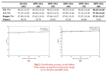
4.4. Comparison with 2D-SSA using all bands
In this section, we analyse the proposed dimensionality reduction algorithm and the original 2D-SSA from the two perspectives of data dimension reduction and the computation time. The original 2D-SSA is used for feature extraction for hyperspectral images using all bands.
In our dimensionality reduction method, the 2D-SSA is applied for feature extraction on a part of bands selected by the proposed band selection method. The results are given as follows.
In Table 5 and Table 6, we analyse the differences in the classification accuracy of the feature extraction with entire bands and the feature extraction with selected bands. The numbers in parentheses indicate the numbers of the selected hyperspectral bands. The numbers of bands for the
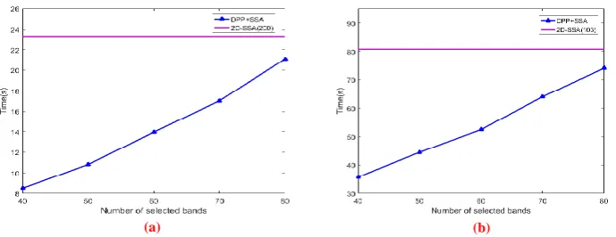
Indian Pines and Pavia University datasets are 200 and 103, respectively. To compare the dimensionality reduction effects of different dimensions, 40 to 80 bands are tested and the dimensionality reduction performances are given with the increment of 10 dimensions each time.
[image:7.595.117.480.394.556.2]8 classification accuracy of our proposed algorithm is very
close to or even slightly higher than the original 2D-SSA. On Pavia University, the experiment results of the two algorithms are similar in terms of classification accuracy, which means that the performance is very close. However, the dimension of dataset extracted by our method is lower and takes much less time. This shows that the features extracted by the original 2D-SSA are partially redundant, and our method can effectively remove the redundancy.
The
reasons why it takes less time are analysed as follows. [image:8.595.114.481.268.337.2]In band selection, the most time consuming is eigen-decomposition of similarity kernel matrix and the construction of adjacency matrix with mutual information. Therefore, we use the Dual-DPP to avoid the decomposition of high-dimensional matrices and reduce the computation time. Besides, we design a method for collecting the spatial representative pixel points with diversity and good coverage. This method avoids the estimation of mutual information on the entire hyperspectral dataset and effectively reduces the calculation time.
Table 5 Classification accuracy and computation time in the Indian Pines image of 2D-SSA and DPP+SSA (Best result of each row is marked in bold type)
2D-SSA (200)
DPP+SSA (40)
DPP+SSA (50)
DPP+SSA (60)
DPP+SSA (70)
DPP+SSA (80) OA (%) 93.09±0.99 92.79±0.85 92.80±0.81 93.17±0.62 93.07±0.94 93.50±0.53 AA (%) 89.25±1.92 89.22±2.01 89.29±2.45 89.56±1.75 89.30±2.24 89.52±1.75
Kappa (%) 92.12±1.13 91.78±0.98 91.79±0.92 92.21±0.70 92.03±1.08 92.59±0.60
Time(s) 23.25 8.47 10.81 13.96 17.02 21.10
Table 6 Classification accuracy and computation time in the Pavia University image of 2D-SSA and DPP+SSA (Best result of each row is marked in bold type)
2D-SSA (103)
DPP+SSA (40)
DPP+SSA (50)
DPP+SSA (60)
DPP+SSA (70)
DPP+SSA (80) OA (%) 98.42±0.23 98.20±0.18 98.23±0.20 98.35±0.25 98.40±0.20 98.43±0.20 AA (%) 97.19±0.38 96.98±0.30 96.92±0.33 97.09±0.46 97.16±0.38 97.20±0.44 Kappa (%) 97.90±0.30 97.62±0.24 97.66±0.27 97.81±0.33 97.87±0.26 97.91±0.27
Time(s) 80.76 35.70 44.45 52.43 64.00 74.02
(b) (a)
Fig.2. Classification accuracy in the Indian Pines image (a) and Pavia University image
[image:8.595.111.479.365.621.2]9
5. Conclusion
In this paper, a new unsupervised dimensionality reduction algorithm is proposed for band selection of hyperspectral image. We make full use of the spatial information of hyperspectral image and construct multiple adjacency matrices to describe the correlation of spectral bands. In addition, we designed a fast spatial sampling method for hyperspectral, collecting some representative sample points, which can effectively reduce the amount of data calculation. An improved k-DPP is presented to sample a diversity and low-redundancy band subset from the multi adjacency matrices. Finally, duo to its ability of extracting features, 2D-SSA is employed and integrated with the improved k-DPP to build our unsupervised dimensionality reduction algorithm which can efficiently extract the spatial features of spectral images.The experimental results on two well-known hyperspectral datasets show that the proposed algorithm achieves higher classification accuracy with effectively compressing the data dimension.
Acknowledgements
This work is supported by the National Nature Science Foundation of China (no. 61471132) and the Training program for outstanding young teachers in higher education institutions of Guangdong Province (no. YQ2015057).
References
[1] W. Li, C. Chen, H. Su, and Q. Du.: ‘Local binary patterns and extreme learning machine for hyperspectral imagery classification,’ IEEE Trans. Geosci. Remote Sens., 2015, 53, (7), pp. 3681-3693
[2] M. Uzair, A. Mahmood, and A. Mian.: ‘Hyperspectral face recognition with spatiospectral information fusion and PLS regression,’ IEEE Trans. Image Process., 2015, 24, (3), pp. 1127-1137
[3] W. Zhao, S. Du.: ‘Spectral-Spatial Feature Extraction for Hyperspectral Image Classification: A Dimension Reduction and Deep Learning Approach,’ IEEE Trans. Geosci. Remote Sens, 2016, 54, (8), pp.4544-4554
[4] G. Reed, K. Savage, D. Edwards, and N. N. Daeidet.: ‘Hyperspectral imaging of gel pen inks: An emerging tool in document analysis,’ Sci. Justice, 2014, 54, (1), pp. 71-80 [5] P. Y. Sacre et al.: ‘Data processing of vibrational chemical imaging for pharmaceutical applications,’ J. Pharmaceutical Biomed. Analy., 2014, 101, pp. 123-140 [6] N. Neittaanmäki-Perttu et al.: ‘Detecting field cancerization using a hyperspectral imaging system,’ Lasers Surgery Med., 2013, 45, (17), pp. 410-417
[7] T. Kelman, J. Ren, and S. Marshall: ‘Effective classification of Chinese tea samples in hyperspectral imaging,’ Artif. Intell. Res., 2013, 2, (4), pp. 87–96 [8] Y. Yuan, X. Zheng, X. Lu.: ‘Discovering Diverse Subset for Unsupervised Hyperspectral Band Selection,’ IEEE Trans. Image Process., 2017, 26, (1), pp. 51-64
[9] J. Feng, L. Jiao, F. Liu, T. Sun, X. Zhang.: ‘Unsupervised feature selection based on maximum information and minimum redundancy for hyperspectral images,’ Pattern Recognit, 2016, 51, pp. 295-309
[10] J. Feng, L. Jiao, F. Liu, T. Sun, and X. Zhang.: ‘Mutual-information based semi-supervise hyperspectral band selection with high discrimination, high information, and low redundancy’, IEEE Trans. Geosci. Remote Sens., 2015, 53, (5), pp. 2956-2969
[11] X. Geng, K. Sun, L. Ji, and Y. Zhao, ‘A fast volume-gradient-based band selection method for hyperspectral image’, IEEE Trans. Geosci. Remote Sens., 2014, 52, (11), pp. 7111-7119
[12] J. Feng, L. C. Jiao, X. Zhang, and T. Sun. ‘Hyperspectral band selection based on trivariate mutual information and clonal selection’, IEEE Trans. Geosci. Remote Sens., 2014, 52, (7), pp. 4092-4105
[13] X.H. Cao, C.C. Wei, J.G. Han, L.C. Jiao.: ‘Hyperspectral Band Selection Using Improved Classification Map,’ IEEE Geosci. Remote Sens. Lett.,2017, 14(11), pp.2147-2151
[14] X.H. Cao, J.G. Han, S.Y. Yang, D.C. Tao, L.C. Jiao.: ‘Band selection and evaluation with spatial information,’ International Journal of Remote Sensing., 2016, 37(19), pp.4501-4520
(b) (a)
Fig.3. Computation time in the Indian Pines image (a) and Pavia University image (b) of
[image:9.595.126.471.134.267.2]10
[15] C. Yao, Y.F. Liu, B. Jiang, J.G. Han, J.W. Han.: ‘LLE Score: A New Filter-Based Unsupervised Feature Selection Method Based on Nonlinear Manifold Embedding and Its Application to Image Recognition,’ IEEE Trans. Image Process., 2017, 26(11), pp.5257-5269
[16] J. M. Sotoca, F. Pla.: ‘Supervised feature selection by clustering using conditional mutual information-based distances’, Pattern Recognit. 2010, 43, (6), pp. 2068-2081 [17] H. Yang, Q. Du, H. Su, and Y. Sheng.: ‘An efficient method for supervised hyperspectral band selection’, IEEE Geosci. Remote Sens. Lett., 2011, 8, (1), pp. 138-142 [18] C. Sui, Y. Tian, Y. Xu, and Y. Xie.: ‘Unsupervised band selection by integrating the overall accuracy and redundancy’. IEEE Geosci. Remote Sens. Lett., 2015, 2, (1), pp. 185-189
[19] C. Wang, M. Gong, M. Zhang, and Y. Chan: ‘unsupervised hyperspectral image band selection via column subset selection.’ IEEE Geosci. Remote Sens. Lett., 2015, 12, (7), pp. 1411-1415
[20] M. Zhang, J. Ma, and M. Gong.: ‘Unsupervised Hyperspectral Band Selection by Fuzzy Clustering With Particle Swarm Optimization’, IEEE Geosci.Remote Sens. Lett., 2017, 14, (5), pp.773-777
[21] C. Gong, D. Tao, S. J. Maybank, W. Liu, G. Kang, and J. Yang.: ‘Multimodal curriculum learning for semi-supervised image classification’, IEEE Trans. Image Process., 2016, 25, (7), pp. 3249-3260
[22] J. Zabalza, J. Ren, J. Zheng, J. Han, H. Zhao, S. Li, S. Marshall.: ‘Novel Two-Dimensional Singular Spectrum Analysis for Effective Feature Extraction and Data Classification in Hyperspectral Imaging,’ IEEE Trans. Geosci. Remote Sens., 2015, 53, (8), pp. 4418-4433 [23] J. Zabalza, J. Ren, J. Zheng, H. Zhao, C. Qing, Z. Yang, P. Du, S. Marshall.: ‘Novel segmented stacked autoencoder for effective dimensionality reduction and feature extraction in hyperspectral imaging,’ Neurocomputing., 2016, 185, pp:1-10
[24]L. Lei, S. Prasad, J.E. Fowler, L.M. Bruce.: ‘Locality-preserving dimensionality reduction and classification for hyperspectral image analysis,’ IEEE Trans. Geosci. Remote Sens., 2012, 50, (4), pp. 1185-1198
[25] B.C. Kuo, C.H. Li, J.M. Yang.: ‘Kernel nonparametric weighted feature extraction for hyperspectral image classification’, IEEE Trans. Geosci. Remote Sens., 2009, 47, (4), pp. 1139-1155
[26] Xiaofei He and Partha Niyogi.: ‘Locality Preserving Projections’, in NIPS, 2003.
[27] M. Belkin and P. Niyogi.: ‘Laplacian eigenmaps and spectral techniques for embedding and clustering,’ in Proc. Av. Neural Inf. Process. Syst.,2001, pp. 585–591.
[28] Y.C. Guo, G.G. Ding, L. Li, J.G. Han, L. Shao.: ‘Learning to Hash With Optimized Anchor Embedding for Scalable Retrieval,’ IEEE Trans. Image Process., 2017, 26(3), pp.1344-1354
[29] G. Licciardi, P. R. Marpu, J. Chanussot, and J. A. Benediktsson.: ‘Linear versus nonlinear pca for the classification of hyperspectral data based on the extended morphological profiles,’ IEEE Geosci. Remote Sens. Lett., 2012, 9, (3), pp.447-451
[30] C. M. Bachmann, T. L. Ainsworth, and R. A. Fusina.: ‘Exploiting manifold geometry in hyperspectral imagery,’ IEEE Trans. Geosci. Remote Sens., 2005, (43), (3), pp. 441– 454
[31] B. Demir and S. Ertürk.: ‘Empirical mode decomposition of hyperspectral images for support vector machine classification,’ IEEE Trans. Geosci. Remote Sens., 2010, 48, (11), pp. 4071–4084
[32] A. Kulesza and B. Taskar.: ‘Determinantal Point Processes for Machine Learning", Foundations and Trends in Machine Learning. 2012, 5, (2-3), pp.123-286
[33] A. Kulesza and B. Taskar: ‘k-DPPs: Fixed-size determinantal point Processes’. in Proc. Int. Conf. on Machine Learning,.2011, pp. 1193-1200
[34] O. Macchi.: ‘The coincidence approach to stochastic point processes,’ Advances in Applied Probability., 1975, 7, (1), pp. 83-122, 1975
[35] T. Cover and P. Hart.: ‘Nearest neighbor pattern classification.’ IEEE Trans. Inf. Theory., 1967,13, (1), pp. 21–27
[36] P. Qiu, A. J. Gentles, S. K. Plevritis.: ‘Fast calculation of pairwise mutual information for gene regulatory network reconstruction’, Comput. Methodsrograms Biomed. 2009, 94, (2), pp.177-180
[37] P. R. Marpu, M. Pedergnana, M. D. Mura, J. A. Benediktsson, and L. Bruzzone,.:‘Automatic generation of standard deviation attribute profiles for spectral–spatial classification of remote sensing data,’ IEEE Geosci. Remote Sens. Lett., 2013.10,(2),pp. 293–297,
[38] R. O. Green, M. L. Eastwood, C. M. Sarture, T. G. Chrien, M. Aronsson, B. J. Chippendale, J. A. Faust, B. E. Pavri, C. J. Chovit, M. Solis, M. R. Olah, O. Williams.: ‘Imaging spectroscopy and the Airborne Visible/Infrared Imaging Spectrometer (AVIRIS).’ Remote. Sens. Environ, 1998, 65, (3), pp. 227-248
[39] S. Holzwarth, A. Müller, M. Habermeyer, R. Richter, A. Hausold, S. Thiemann,P. Strobl,Sens - DAIS 7915 / ROSIS Imaging Spectrometers at DLR, in: 3rd EARSeL Workshop on Imaging Spectroscopy, Herrsching,13-16 May 2003, p. 12
[40] Y. Bazi, F. Melgani.: ‘Toward an optimal SVM classification system for hyper-spectral remote sensing images,’ IEEE Trans. Geosci. Remote Sens, 2006, 44, (11) pp. 3374–3385