The effect of bathymetry interaction with waves and sea currents on the loading and thrust of a tidal turbine

The effect of bathymetry interaction with waves and

sea currents on the loading and thrust of a tidal

turbine.

Jose Manuel Rivera Camacho

, Cameron M. Johnstone

, Stephanie E. Ordonez Sanchez

16 Richmond St. Glasgow G1 1XQ, Scotland. U.K.

1_{[email protected]} 2_{[email protected]}

3_{[email protected]}

Abstract— this paper reports work undertaken to advance analytical methods used to evaluate the influence of bathymetry on wave- current interactions with tidal turbines. The model takes in to account the wave transformation due to a sudden depth change in the sea level. The functions developed provide solutions for wave transformation by changes in bathymetry to find how this change effects the torque and thrust exerted over a tidal turbine. Costal site data for the west coast of the US, from the US DoE, has been used to access the robustness of these analytical methods. The high resolution data sets used have monitored wave, sea and climatic conditions over a period of 8 years.

Keywords— Bathymetry, Tidal Turbine, BEMT, Waves, Swell conditions.

I. INTRODUCTION

Tidal energy has been evolving since the firsts in-sea deployed prototypes were undertaken in the early 2000’s. Over this period, a diverse range of design configurations has been proposed, however the most dominant technology architecture is the horizontal axis turbine. These devices feed on the research undertaken the wind turbine industry and experiences gained through the commercialisation of wind farms. However, the environmental difference between sea and air makes the final design of tidal turbines different. The higher density of the water, the highly corrosive medium, the lower flow velocities and the perturbation on the velocity field due to waves and turbulence in the flow are just some of the main differences.

Regarding these differences, waves are one of the main sources of high variable loads experienced on tidal turbines. The orbital motion of the water particles as they pass creates a changing circular or ellipsoidal velocity field from the sea surface to the sea bed. This field will interact with the turbine rotor and produce a cyclical variation on the thrust and torque on each cycle, e.g. [1], [2] and [3]. This load variation will affect the mechanical loading and energy performance of the power capture interface and the components of the power transfer system [4].

Another important factor that could affect the wave loads is the sites geographical installation of the turbine, not only the surrounding area, but also the depth. The influence of waves velocity on the current flow can reach a depth equal to half of the wavelengths 𝑑 <l

# [5], so depending on the water depth of

the installation, wave disturbance on flow velocity can vary. Larger wavelengths will penetrate deeper into the water column. Swell waves will become the dominant component of spectrum in deeper waters, while a combination of swell waves and local wind waves will influence the spectrum at medium and shallow waters. The structure of the swell wave alter as they near the coast, with the existence of sea bed obstacles and the decrease in water depth being the two main factors for this. Previous studies have shown both analytically and experimentally [6], [7], [8], [9] and [10] how swell waves can be transmitted and reflected against obstacles on the sea bed. Most of these studies have been focused on linear waves, which have a smaller amplitude in relation to their wavelength, 𝑎 ≪ l . Studies have shown how the changes in amplitude, frequency and the generation of harmonics in the wave spectrum vary depending on changes in the obstacle depth ratio, obstacle length and incoming wavelength [8], [9] and [10].

In developing an understanding of the differences in turbine operating performance, this paper investigates the changes in torque and thrust to be experienced in a tidal turbine before and after swell has been encountered from a change in bathymetry. The data used has been extracted from instrumented buoys operating under the NDBC (National Data Buoy Centre) of San Francisco Bay, on the west coast of the US. A bathymetry cross section from west to east of the California coast was taken as a representation of a ‘regular’ bathymetry change and used as an input to the model. Eight years worth data for two buoys operating in the area was used to identify a function which defines the frequency change of the bathymetry section chosen, the 1st _{Buoy 46214 installed at a depth of 550m and the 2}nd

46026 installed at 54.9m. Matlab was used to process and select only swell wave conditions and correlate, via time series, the west site (open sea swell) to the east site (swell in shallower water). The results from the encountered function were then fed into a BEMT model using a NREL S814 blade profile to obtain the thrust and torque for turbine operations before and after the idealized bathymetry change.

II. MODEL

The place to be modelled is known for being exposed to seasonal swells coming mainly from the south/southwest in the months of May to September and the west/northwest in the months of October to April [12]. The Bathymetry information used on the report comes from the USGS (United States Geological Survey) [13], data was processed in to QGIS to have a 2D map of the elevation in the surrounding sea to obtain a geographical place for the bathymetry cut.

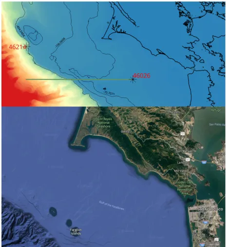
The place was chosen cause of its more regular bathymetry change from open sea to shallow waters and cause the spring/summer swell has a mostly perpendicular incidence at the coast. The cut chosen ranges from 84km open sea in the west coast of California to 28km the coast of the state, following the line of the latitude 37.755o_{. Swell modelled here}

comes from the west-east direction, we can see the place more detailed on Fig. 1 and Fig. 2.

Fig. 1 The section of the bathymetry profile chosen for modelling, capturing the west swell of the north pacific. The figure shows points A and B, where B sits on the near end of the shelf at approximately 71 m depth.

Fig. 2 The cut on the bathymetry profile chosen is shown in green with the biggest differences on the bathymetry change on black lines, the buoys used are the 46214 and 46026 shown in the map. Another version of the map with complete features is shown in the part below.

files are made available to the public [14] and the data report informs users where the data set was gathered, the main characteristics during that time. The structure of the most important data used in these files is explained in table 1:

Label Meaning units

YY Year none

MM Month none

DD Day none

HH Hour none

Mm minute none

WDIR Wind direction degrees

WVHT Wave wind height m

DPD Dominant period s

APD Average period s

MWD Mean wave direction degrees

TIDE Tide meters

Table 1.- Data in the text files at the NDBC website contains the main characteristics of the sea, averaged every 30 minutes, In these, the wave conditions, wind conditions and weather conditions are recorded. However, not all the data is used, wind speed and wind direction is not considered in order to avoid increasing model complexity at this moment.

The first set of data used is the DPD (wave dominant period) was mean wave direction from the buoy number 46214. According to the NDBC, the DPD is the more energetic period of the wave spectrum and the MWD is the average direction from which this period comes from. These data files are used to feed the code. The data was filtered and analysed to search for linear conditions form the west direction. If the necessary governing conditions are met {T>10s, direction 270o_±11.25o_}

and if is linear [5], the wavelength and the wave group velocity are calculated and stored in a text file. Matlab also relates the conditions of the swell from buoy 46214 to the swell arriving to buoy 46026 in search of a swell that corresponds to the one that already passed from the 1st buoy, the general work of the code can be seen at Fig. 3 and Fig. 4.

Fig. 3 The script searches for swell conditions at the two buoys, these conditions must also be linear in order for the theory to work. The wave must come from the east direction (270 ± 11.25o _{north/south) . Suitable data series}

are stored to a file recording the conditions at that time.

Fig. 4 This program compares both swells waves at points A and B, if the conditions in point B match the conditions in time A we can say they are part of the same swell and the Frequency change in the swell is calculated.

If we plot a 3D probability histogram showing where wave frequency changes cluster, the heights of the wave and the number of measurements within the data stream, we get figure 5.

Fig. 5 The figure shows how the Cw that is the ratio between the transmitted frequency and the incoming frequency changes and groupings depending on the period of the incoming wave.

The frequency changes are gathered in to packed groups, then divided in to a 2D representations to fit a function which describes their behaviour around this particular bathymetry section during the 8 years period of data. From Fig. 4, The function describing the swell behaviour has the form

f(x) = a + b (x)1/2

Fig. 6 The plot identifies the best approximation for the function. This describes the route through the more dense set of data, from left to right the periods are: 10.53, 11.11, 11.76, 12.50, 13.13, 14.29, 15.38, 16.67, 18.18, 20.00 and 22.22 seconds. The red lines show the regions with small period change from 12.5s to 15.38s.

The function at that bathymetry change is coupled with solutions for the wave amplitude transmission [15], these solutions are obtained using linear theory. This solution is of the form shown in equation 1:

1

Kr, our reflection coefficient will have the form shown below at equation 2:

2

Here 𝜀 = 4𝑠*𝜋𝑁, 𝑠*= ℎ. ℎ/ , 𝑠0= ℎ1 ℎ/ , 𝑁 =2#32₅ 4; we can see the depths and the distances in fig. 7.

Fig. 7 The bathymetry section modelled can be generalized from the jumps as

ℎ.~400𝑚, ℎ/~191𝑚 and ℎ1~71𝑚. The distance between 𝑥/ and 𝑥1is almost

4km (3970m).

The frequency change and amplitude change functions are used to obtain the torque and thrust variation on a turbine at points A and B, swell conditions are complemented by localised wind conditions, as taken from both buoys. At point A, we expect swell conditions be similar to that of the open sea due to the closeness to the continental slope and the specific abrupt change in bathymetry in this zone.

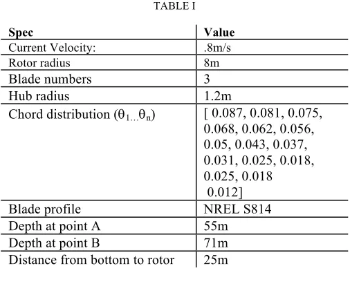
The turbine rotor and the conditions used can be seen in table 1:

TABLE I

Spec Value

Current Velocity: .8m/s

Rotor radius 8m

Blade numbers 3

Hub radius 1.2m

Chord distribution (q1…qn) [ 0.087, 0.081, 0.075,

0.068, 0.062, 0.056, 0.05, 0.043, 0.037, 0.031, 0.025, 0.018, 0.025, 0.018 0.012]

Blade profile NREL S814

Depth at point A 55m

Depth at point B 71m

Distance from bottom to rotor 25m

III.CASES

Two cases are used to model the behaviour of swell waves on to the rotor, the first is a swell only component with 19.05s period at points A and B; the second one is combination of swell with long wavelength of 19.05s period, swell of short wavelength with 10.5s period and normal wind waves with 6.2s period. In all cases wave height is less than 2m with data taken from particular cases during 2017.

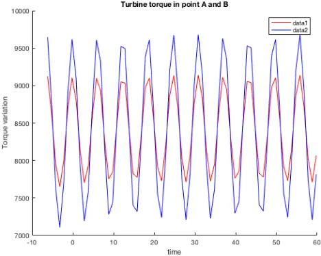
A. Torque and thrust on point A (Red) and B (Blue) under swell conditions:

In this case, a swell of 19.01s is chosen from the data of 2017, a steady current of .8m/s is placed across our turbine.

Fig. 5 shows the overall torque change at the rotor, the blue indicates how the swell disturbance is damped by the change in the sea elevation from point A to B, data 1 is the torque at site A and data 2 on site B.

Re[eik0x−_kreik0x_]=η_(x)

T

kr=

(sa−sb)

2₊(1−sb

2

)(1−sa

2

)(1−Cos(ε)) 2

(sa+sb)

2₊(1−sb

2

)(1−sa

2

Fig. 6 The plot shows the overall thrust change at the rotor, the blue indicates how the swell disturbance is damped by the change in the sea elevation from point A to B,, data 1 is the torque of on the site A and data 2 on site B.

B. Torque and thrust on point A (red) and B (blue) under mixed conditions with swell of long period, short period and wind waves.

In this case, a swell of 19.01s along with a swell of 10.5s and wind waves of 6.2s are chosen from the data of 2017, a steady current of .8m/s is placed across our turbine.

Fig. 7 shows the overall thrust change at the rotor, here the complex interaction between the three conditions show a different output for torque and thrust, with data 1 being the torque of on the site A and data 2 on site B.

Fig. 8 The plot shows the overall thrust change at the rotor, here the complex interaction between the three conditions shows a different output at the torque and thrust., data 1 is the torque of on the site A and data 2 on site B.

IV.CONCLUSIONS

As demonstrated, both the torque and thrust are affected by the wave transformation associated with bathymetry changes. These increases the values when the turbine is under swell conditions only at site A. This could be due to exposure to the swell energy before reaching the continental shelf. The same occurs for the thrust, as expect. The results from the mixed combination, swell and local wind driven waves, is more complex. This shows exactly the opposite behaviour, which could suggest wind waves and short swell waves are able to pass through the shelf with little/ no modification. Despite of the results of the mixed case, it could be expected that the function found after fitting the data depends greatly on the depth ratio between the ocean bottom and the regular bathymetry change. However, more data is needed in order to verify such a dependency.

Future work will see experiments carried out at scale and in a controllable large test facility in order to find a dependency on this function and to be able to model other bathymetry changes knowing the function constant dependency.

REFERENCES

[1] S.C. Tatum, C.H. Frost, M. Allmark, D.M. O’Doherty, A. Mason-Jones, P.W. Prickett, R.I. Grosvenor, C.B. Byrne, T. O’Doherty. Wave- current interaction effects on tidal strea, turbine performance and loading characteristics, International journal of Marine Energy, Vol 14, pp. 161-179, June 2016. [2] D. Markus, R. Wuchner, K.U. Bletzinger. A numerial

investigation of combined wave-current loads on tidal stream generators, Vol 72, pp. 416-428, November 2013.

[3] P. Ouro, H. Magnuss, S. Thorsten, P. Bromley. Hydrodynamic loadings on a horizontal axis tidal turbine prototype, Journal of Fluids and Structures, vol 71, pp. 78-95, May 2017.

[5] A. Pecher, J.P. Kofoed, Handbook of Ocean Wave Energy, Ed. Springer, 2017.

[6] H. Lamb, Hydrodynamics, 6th ed., Ed. New York, U.S.A: Dover 1945.

[7] J. Newman, Propagation of water waves over an infinite step, Journal of Fluid Mechanics, vol. 23, pp. 399-415, April 1965. [8] M. Christou, C. Swan, O. Gudmestand, The interaction of water

surface waves with submerged breakwaters, Coastal Engineering, vol. 45, pp. 945-958, December 2008.

[9] F. Seabra-Santos, D. Renouard, A. Temperville, M. Andre, Numerical and experimental study of the transformation of a solitary wave over a shelf or isolated obstacle. Journal of Fluid Mechanics, vol. 176, pp. 117-134, April 2006.

[10] D.G. Goring, “Tsunamis-The propagation of long Waves onto a Shelf”, PhD. Civil Eng. thesis, California Institute of Technology, Pasadena, USA, Nov 1978.

[11] (2014), The Atlantis Resources website. [Online]. Available:

https://simecatlantis.com.

[12] S. Peak, “Wave Refraction over Complex Nearshore Bathymetry”, M. Science. thesis, Naval Posgraduate School, Monterey, USA, Sep 2004.

[13] (2018), USGS online webpage. [Online]. Available: https://sfbay.wr.usgs.gov/sediment/sfbay/index.html

[14] (2018), NDBC online webpage. [Online]. Available:

https://www.ndbc.noaa.gov