Rochester Institute of Technology
RIT Scholar Works
Theses Thesis/Dissertation Collections
2013
Implementing a dynamic scaling of web
applications in a virtualized cloud computing
environment
Mohammed Aljebreen
Follow this and additional works at:http://scholarworks.rit.edu/theses
This Thesis is brought to you for free and open access by the Thesis/Dissertation Collections at RIT Scholar Works. It has been accepted for inclusion in Theses by an authorized administrator of RIT Scholar Works. For more information, please [email protected].
Recommended Citation
Rochester Institute of Technology
Golisano College of Computing and Information Sciences
Dept. of Networking, Security, & Systems Administration
Implementing a Dynamic Scaling of Web Applications
in a Virtualized Cloud Computing Environment
By
Mohammed Aljebreen
Committee Chair:
Professor Sharon Mason
Committee Members:
Professor Larry Hill Professor Jim Leone
Thesis submitted in partial fulfillment of the requirements for the degree
of Master of Science in
Networking and System Administration
Rochester Institute of Technology
B. Thomas Golisano College of Computing and Information Sciences
Abstract
Cloud computing is becoming more essential day by day. The allure of the
cloud is the significant value and benefits that people gain from it, such as reduced
costs, increased storage, flexibility, and more mobility. Flexibility is one of the major
benefits that cloud computing can provide in terms of scaling up and down the
infrastructure of a network. Once traffic has increased on one server within the
network, a load balancer instance will route incoming requests to a healthy instance,
which is less busy and less burdened. When the full complement of instances cannot
handle any more requests, past research has been done by Chieu et. al. that presented
a scaling algorithm to address a dynamic scalability of web applications on a
virtualized cloud computing environment based on relevant indicators that can
increase or decrease servers, as needed. In this project, I implemented the proposed
algorithm, but based on CPU Utilization threshold. In addition, two tests were run
exploring the capabilities of different metrics when faced with ideal or challenging
conditions. The results did find a superior metric that was able to perform
Dedication
I lovingly dedicate this thesis to my gracious and devoted mother for her unwavering
Acknowledgments
This thesis would not have been possible without the support of many people.
My wish is to express humble gratitude to the committee chair, Prof. Sharon Mason,
who was perpetually generous in offering her invaluable assistance, support, and
guidance. Deepest gratitude is also due to the members of my supervisory committee,
Prof. Lawrence Hill and Prof. Jim Leone, without whose knowledge and direction this
study would not have been successful. Special thanks also to Prof. Charles Border for
his financial support of this thesis and priceless assistance.
Profound gratitude to my mother, Moneerah, who has been there from the
very beginning, for her support and endless love. I would also like to convey thanks to
my wife for her patient and unending encouragement and support throughout the
duration of my studies; without my wife’s encouragement, I would not have
completed this degree. I wish to express my gratitude to my beloved sister and
brothers for their kind understanding throughout my studies. Special thanks to my
Table of Contents
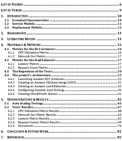
LIST OF FIGURES ... 6
LIST OF TABLES ... 9
1. INTRODUCTION ... 10
1.1 Essential Characteristics: ... 10
1.2 Service Models: ... 11
1.3 Deployment Models: ... 11
2. BACKGROUND ... 13
3. LITERATURE REVIEW ... 13
4. MATERIALS & METHODS: ... 15
4.1 Metrics for the EC2 instances: ... 16
4.1.1 CPU Utilization Metric: ... 16
4.1.2 Network Out Metric: ... 17
4.2 Metrics for the load balancer: ... 17
4.2.1 Latency Metric: ... 17
4.2.2 Request Count Metric: ... 17
4.3 The Repetition of the Tests: ... 20
4.4 The project’s architecture: ... 22
4.4.1 Launching Amazon EC2 instances: ... 22
4.4.2 Creating an Amazon Machine Image (AMI): ... 31
4.4.3 Creating an Amazon Load Balancer: ... 32
4.4.4 Configuring Amazon Auto Scaling: ... 35
4.4.5 Creating CloudWatch Alarms: ... 41
5. DEMONSTRATIONS & RESULTS: ... 45
5.1 Auto Scaling Testing: ... 45
5.2 Tests’ Results: ... 47
5.2.1 CPU Utilization Metric Results: ... 48
5.2.2 Network Out Metric Results: ... 55
5.2.3 Latency Metric Results: ... 62
5.2.4 Request Counts Metric Results: ... 69
5.2.5 Discussion: ... 76
6. CONCLUSION & FUTURE WORK ... 81
7. REFERENCES ... 82
[image:6.595.87.506.111.596.2]LIST OF FIGURES
Figure Page
1.1 Typical Cloud Computing Environment 12
4.1 Dynamic Scaling Algorithm for Virtual Machine Instances in the Cloud 16 4.1.1 Policies of scaling up and down for all tested metrics as shown in AWS management console 18 4.2 Architecture to Scale Web Applications in a Cloud 22 4.3 Amazon Web Services Management Console 23
4.4 Amazon EC2 Console Dashboard 23
4.5 Create a New Instance page 24
4.6 Choose the AMI from the Quick Start tap 25 4.7 Choose the number and the type of the instance 25
4.8 Naming the instance 26
4.9 Key pair creation 26
4.10 Security Group Creation 27
4.11 The web server instance 27
4.12 The web server started 28
4.13 Apache2 included in the instance services 28
4.14 Apache Service Monitor 29
4.15 The home web page of the website 31
4.16 The AMI from the web server 32
4.17 Web server Load Balancer 33
4.18 The servers under the load balancer 33
4.19 Adding Webserver (1) & (2) to the Load Balancer 33 4.20 Advanced Options of the load balancer’s configuration 34 4.21 Java version 1.7 installed on the web server 35 4.22 Testing the Auto Scaling command line installation 36
4.23 MyAutoConfig creation 37
4.24 MyGroup2 creation 39
4.25 Verifying the Auto Scaling Group creation 39
4.26 Verifying the Auto Scaling instances 39
4.27 Scale Up Policy 40
4.28 Scale Down Policy 41
4.29 Testing the CloudWatch command line installation 42
4.30 HighCPU-alarm 43
4.31 LowCPU-alarm 43
4.32 The alarms of the CloudWatch in AWS management console 44
5.1 Auto Scaling creates an instance 45
5.2 CloudWatch Alarms 46
5.3 A notification email in [email protected] inbox 46
5.4 Shutting the temporary instance down 47
5.5 Terminating the temporary instance 47
CPU Utilization Metric’s results for the first test
5.1.1 Weekday mornings at RIT System Lab 48
5.1.2 Weekday evenings at RIT System Lab 49
5.1.3 Weekend mornings at RIT System Lab 49
5.1.4 Weekend evenings at RIT System Lab 49
5.1.5 Weekday mornings from home 49
5.1.6 Weekday evenings from home 50
5.1.7 Weekend mornings from home 50
5.1.9 From a server within Amazon datacenter in Virginia web server 50
5.1.10 From a server within Amazon in Oregon 51
5.1.11 From a server within Amazon in Northern California 51
CPU Utilization Metric’s results for the second test
5.2.1 Weekday mornings at RIT System Lab 52
5.2.2 Weekday evenings at RIT System Lab 52
5.2.3 Weekend mornings at RIT System Lab 52
5.2.4 Weekend evenings at RIT System Lab 53
5.2.5 Weekday mornings from home 53
5.2.6 Weekday evenings from home 53
5.2.7 Weekend mornings from home 53
5.2.8 Weekend evenings from home 54
5.2.9 From a server within Amazon datacenter in Virginia web server 54
5.2.10 From a server within Amazon in Oregon 54 5.2.11 From a server within Amazon in Northern California 55
Network Out Metric’s results for the first test
5.3.1 Weekday mornings at RIT System Lab 56
5.3.2 Weekday evenings at RIT System Lab 56
5.3.3 Weekend mornings at RIT System Lab 56
5.3.4 Weekend evenings at RIT System Lab 56
5.3.5 Weekday mornings from home 57
5.3.6 Weekday evenings from home 57
5.3.7 Weekend mornings from home 57
5.3.8 Weekend evenings from home 57
5.3.9 From a server within Amazon datacenter in Virginia web server 58
5.3.10 From a server within Amazon in Oregon 58
5.3.11 From a server within Amazon in Northern California 58
Network Out Metric’s results for the second test
5.4.1 Weekday mornings at RIT System Lab 59
5.4.2 Weekday evenings at RIT System Lab 59
5.4.3 Weekend mornings at RIT System Lab 60
5.4.4 Weekend evenings at RIT System Lab 60
5.4.5 Weekday mornings from home 60
5.4.6 Weekday evenings from home 60
5.4.7 Weekend mornings from home 61
5.4.8 Weekend evenings from home 61
5.4.9 From a server within Amazon datacenter in Virginia web server 61
5.4.10 From a server within Amazon in Oregon 61
5.4.11 From a server within Amazon in Northern California 62
Latency Metric’s results for the first test
5.5.1 Weekday mornings at RIT System Lab 63
5.5.2 Weekday evenings at RIT System Lab 63
5.5.3 Weekend mornings at RIT System Lab 63
5.5.4 Weekend evenings at RIT System Lab 63
5.5.5 Weekday mornings from home 64
5.5.6 Weekday evenings from home 64
5.5.7 Weekend mornings from home 64
5.5.8 Weekend evenings from home 64
5.5.9 From a server within Amazon datacenter in Virginia web server 65
5.5.10 From a server within Amazon in Oregon 65
5.5.11 From a server within Amazon in Northern California 65 Latency Metric’s results for the second test
5.6.1 Weekday mornings at RIT System Lab 66
5.6.2 Weekday evenings at RIT System Lab 66
5.6.3 Weekend mornings at RIT System Lab 66
5.6.4 Weekend evenings at RIT System Lab 67
5.6.6 Weekday evenings from home 67
5.6.7 Weekend mornings from home 67
5.6.8 Weekend evenings from home 68
5.6.9 From a server within Amazon datacenter in Virginia web server 68
5.6.10 From a server within Amazon in Oregon 68
5.6.11 From a server within Amazon in Northern California 69
Request Counts Metric’s results for the first test
5.7.1 Weekday mornings at RIT System Lab 70
5.7.2 Weekday evenings at RIT System Lab 70
5.7.3 Weekend mornings at RIT System Lab 70
5.7.4 Weekend evenings at RIT System Lab 70
5.7.5 Weekday mornings from home 71
5.7.6 Weekday evenings from home 71
5.7.7 Weekend mornings from home 71
5.7.8 Weekend evenings from home 71
5.7.9 From a server within Amazon datacenter in Virginia web server 72
5.7.10 From a server within Amazon in Oregon 72
5.7.11 From a server within Amazon in Northern California 72
Request Counts Metric’s results for the second test
5.8.1 Weekday mornings at RIT System Lab 73
5.8.2 Weekday evenings at RIT System Lab 73
5.8.3 Weekend mornings at RIT System Lab 74
5.8.4 Weekend evenings at RIT System Lab 74
5.8.5 Weekday mornings from home 74
5.8.6 Weekday evenings from home 74
5.8.7 Weekend mornings from home 75
5.8.8 Weekend evenings from home 75
5.8.9 From a server within Amazon datacenter in Virginia web server 75
5.8.10 From a server within Amazon in Oregon 75
5.8.11 From a server within Amazon in Northern California 76
LIST OF TABLES
Table Page
1. INTRODUCTION
Over the years, the National Institute of Standards and Technology (NIST) has
worked on defining cloud computing. In November 2009, the first draft of a cloud
computing definition was created. The NIST has recently published the 16th and final
draft. According to the NIST definition, "cloud computing is a model for enabling
ubiquitous, convenient, on-demand network access to a shared pool of configurable
computing resources (e.g., networks, servers, storage, applications and services) that
can be rapidly provisioned and released with minimal management effort or service
provider interaction."[3]
The NIST states that the cloud model is composed of five essential
characteristics, three service models, and four deployment models. [4]
1.1Essential Characteristics:
1.1.1 On-demand self-service: A consumer can be provided with computing
capabilities, such as a server and storage, as needed without interaction
with a cloud provider.
1.1.2 Broad network access: Capabilities are available over the network from
anywhere via different platforms such as laptops, mobiles, PCs, etc.
1.1.3 Resource pooling: The resources of the cloud provider are pooled to serve
customers.
1.1.4 Rapid elasticity: The resources can be elastically provisioned. Also, they
appear to the consumer to be unlimited and can be provided at any time.
1.1.5 Measured service: The cloud provider and its consumer can monitor usage
of the resources and control aspects such as storage, processing, active
1.2Service Models:
1.2.1 Cloud Software as a Service (SaaS): The capability of using the provider's
applications running on a cloud infrastructure. The provider is responsible
for managing the underlying cloud infrastructure.
1.2.2 Cloud Platform as a Service (PaaS): The capability given to the consumer
for deploying acquired applications onto the cloud infrastructure using
tools supported by the provider.
1.2.3 Cloud Infrastructure as a Service (IaaS): The capability given to the
consumer to get storage, networks, and other computing resources that the
consumer can deploy, which includes any software, whether operating
system or application.
1.3Deployment Models:
1.3.1 Private cloud: In this model, the infrastructure of the cloud can be only
operated for an organization, and it can be managed by the organization
itself or by a third party.
1.3.2 Community cloud: In this model, the cloud infrastructures are shared
between certain organizations, which support a certain community that has
shared concerns.
1.3.3 Public cloud: Here, the infrastructure is available to the public and is
owned by a certain organization that sells services.
1.3.4 Hybrid cloud: Here in this model, two or more clouds (private,
Figure 1.1: Typical Cloud Computing Environment [2]
As many organizations and industries are moving toward having their work
done in the cloud, cloud computing becomes more essential day by day. The allure of
the cloud is the significant value and benefits that people gain from it, such as reduced
costs, increased storage, flexibility, and more mobility [1]. Flexibility is one of the
major benefits that cloud computing can provide in terms of scaling up and down the
infrastructure of a network. For example, when a server receives a glut of requests
and cannot handle such demands, a new server will be added to help handle these
requests. Chieu et. al. [2] presented a scaling scenario to address the dynamic
scalability of web applications on a virtualized cloud computing environment. The
scenario is based on using a load balancer to route user requests to web servers that
provide web service. The load balancer routes incoming requests to servers that host
the web application. The question is: what if the full complement of instances cannot
handle more requests? Chieu et. al. proposed a dynamic scaling algorithm that the
number of the instances should automatically scale based on the threshold on the
2. BACKGROUND
Cloud computing history dates to the 1960s, when McCarthy posited his idea
that “computation may someday be organized as a public utility” [5]. The concept of
cloud computing was taken from telecommunications companies in the 1990s,
making a radical shift from point-to-point data circuits to Virtual Private Network
(VPN) services. The term “cloud computing” was used academically for the first time
in 1997 by Professor Chellappa in a lecture titled “Intermediaries in
Cloud-Computing”. He suggested that this would be a new "computing paradigm where the
boundaries of computing will be determined by economic rationale rather than
technical limits alone."1
Companies began to move to the cloud as early as 1999. Salesforce.com was
one of the first. The company introduced the concept of “delivering enterprise
applications via a simple website” [5]. In 2002, Amazon.com launched Amazon Web
Services [6]. Google Docs came next, in 20062. Eucalyptus came in 2008, and was the
first open source option for deploying a private cloud. Microsoft entered the cloud by
launching Microsoft Azure in 2009. Today, there are many companies involved in
cloud computing solutions, such as Oracle, Dell, IBM, Fujitsu, Teradata, and HP [5].3
3. LITERATURE REVIEW
Mao et. al [7] presented a mechanism that dynamically scales cloud
infrastructure up and down based on deadline and budget information. The proposed
mechanism scales using a virtual machine (VM) that takes into consideration the
performance and budget of the application. In terms of the performance, the
mechanism provides enough VM instances to finish submitted jobs within the defined
1 From his personal website: http://www.bus.emory.edu/ram/
2 Google Docs belongs to a Software as a Service (SaaS) under the service models.
deadline. In terms of budget, the mechanism runs VM types4 based on the
applications’ needs. For example, if the submitted job does not need a huge processor,
the mechanism will provide a small VM type instead of a large one, and vice versa.
This mechanism could cut costs when compared to using only one type of instance.
Cushing et. al. [8] proposed a method for auto scaling data-centric workflow
tasks using a prediction-based approach. The authors achieved scaling using a
prediction mechanism in which the input data load on a workflow's task is used to
compute the estimated time for execution of the task. Through this prediction, a
framework can make decisions to scale multiple tasks independently to improve
output and reduce congestion.
Dean. et. al [9] developed a programming model called MapReduce which
more closely relates to this project. MapReduce is a software framework—introduced
by Google—which supports distributed computing on large data sets on computer
clusters [18]. MapReduce processes data that is distributed across servers in a cluster
using three operations [19]. The first is called Map, which is a set of tasks that process
in parallel by each node within a cluster separated from other nodes within that
cluster. Users determine a map function, which processes a key/value pair to generate
a set of intermediate key/pair values [9]. Every map task is assigned a part of the input
file that is called a split. Each split has a single HDFS block by default [20]. The
second involves data that is distributed across all nodes within the cluster, and the
third, known as reduce, is a set of tasks that each node executes in parallel. Here, the
values that are associated with same key are merged.
Venugopal et. al [8] used features of the Session Initiation Protocol (SIP), in addition
to using the Amazon Elastic Compute Cloud service (EC2), to implement a
mechanism which scales a VoIP-based call center to respond to emergency calls.
4 For example, Amazon Elastic Compute instances (EC2) are grouped into seven groups of types [13]:
They developed a control system that dynamically scales up or down according to the
increasing or decreasing call volumes. Their results show that the control system was
able to respond to increasing call volumes by providing additional severs as needed.
4. MATERIALS &METHODS:
The algorithm proposed (see figure 4.1) in the paper titled “Dynamic Scaling of Web
Applications in a Virtualized Cloud Computing Environment” written by Chieu at. al,
[2] uses the number of active sessions in each server to scale up and down as a
threshold. However, in this thesis, the same algorithm has been implemented on an
Figure 4.1: Dynamic Scaling Algorithm for Virtual Machine Instances in the Cloud. [1]
The CPU utilization metric will be used as an example for how to set auto scaling for
practical purposes (see section 4.1.4), however the actual experiment will be done
without auto scaling action and will compare several metrics to decide which is the
most effective. These tests (explained below in the Tests’ Results Section) would be
performed through various substantial analyses.
When debating which metrics to use, those of the load balancer should also be taken
into consideration as well as the EC2 Instances. Thus, a Network Out metric would be
used as a metric of the EC2 instances besides the CPU Utilization metric. In regards
to the load balancer metrics, two metrics were chosen: Latency and Request Count.
The explanation of each metric is as follows:
4.1Metrics for the EC2 instances:
4.1.1 CPU Utilization Metric:
As explained earlier, this is the percentage of an “allocated EC2 [which] computes
units that are currently in use on the instance. This metric identifies the processing
power required to run an application upon a selected instance.”5
4.1.2 Network Out Metric:
“The number of bytes sent out on all network interfaces by the instance. This metric
identifies the volume of outgoing network traffic to an application on a single
instance.”3
4.2Metrics for the load balancer:
4.2.1 Latency Metric:
“Time elapsed after the load balancer receives a request until it receives the
corresponding response.”3
4.2.2 Request Count Metric:
“The number of requests handled by the load balancer.”3
Due to the huge variety of applications, website workloads, and web servers type,
there is no universal policy for when a certain metric should be scaled. The policies
featured below in Table 1 were created through tests using an experimental website,
T1.micro type:
Metric Policy of Scaling Up Policy of Scaling Down
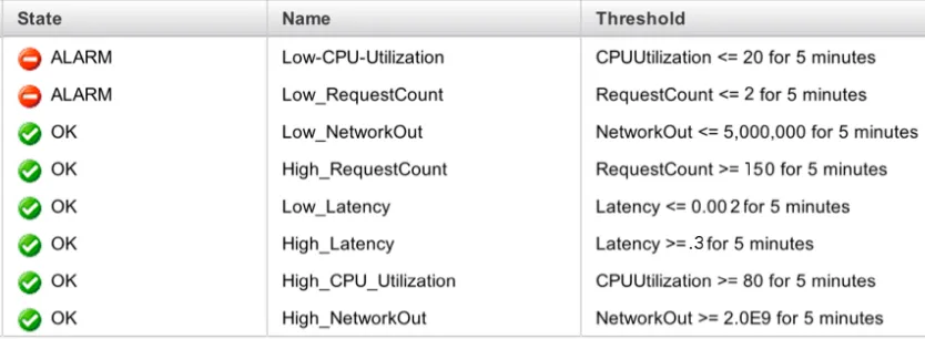
CPU Utilization CPU Utilization >= 80 % for 5 minutes
CPU Utilization <= 20 % for 5 minutes
Network Out Network Out >= 2 GB for 5 minutes Network Out <= 5 MB for 5 minutes
Latency Latency >= 0.3 second for 5 minutes Latency <= 0.002 second for 5 minutes
Request Count Request Counts >= 150 requests for 5 minutes
Request Counts <= 2 requests for 5 minutes
Figure 4.1.1: Policies of scaling up and down for all tested metrics as shown in AWS management console
Since the metrics differ in how they reach their upper and lower boundaries, two tests
had to be performed to ensure proper results. The first test, designed specifically for
the EC2 instances metrics (CPU Utilization & Network Out), involves three users
running a bash script that downloading a gallery of photos (sized 1.6 GB) from the
T1Micro server. The script has two loops: the outer loop runs 5 times, with the inner
loop running twice per outer loop. When the inner loop runs, it starts by downloading
the gallery. When the download is finished, it stops for two minutes, before repeating
the process. When the loop is completed, it stops for seven minutes, after which the
second loop of the outer loop would start. This test, called FIRST TEST, is in the
The second test, coded for the Load Balancer metrics (Latency & Request Count),
involves a bash script that downloads the index page (3KB). The bash script also has
two loops, with the outer loop running 100 times, and the inner running 30 times per
outer loop. When the inner loop runs, it downloads the index page thirty times, with a
one-second waiting period between each connection. When completed, it stops for 15
seconds before the second loop of the outer loop starts. This continues until the end of
the script. This test is called SECOND TEST, and can also be found in the results
sections. Below is the bash script: #!/bin/bash
START=$(date +%s.%N)
command
counting=0;
for i in {1..5}
do
for j in { 1..2}
do
wget myloadbalancer-1942790311.
us-east-1.elb.amazonaws.com/Photos.gz;
sleep 2m;
let "counting += 1";
done
sleep 7m;
echo "$counting of galleries have been downloaded";
done
END=$(date +%s.%N)
DIFF=$(echo "$END - $START" | bc)
echo $DIFF
4.3The Repetition of the Tests:
The tests were conducted multiple times in different times and places to better
compare the metrics. Five different locations were chosen. The first was in a home
setting, since this is where most people access the Internet. The second was in the
Systems Lab in Golisano College of Computing and Information Sciences at
Rochester Institute of Technology. This location offered vastly different results than #!/bin/bash
START=$(date +%s.%N)
command
counting=0;
for i in {1..100}
do
for j in {1..30}
do
wget myloadbalancer-1942790311.
us-east-1.elb.amazonaws.com/index.html;
sleep 1;
let "counting += 1";
done
echo "$counting times I connected to the
loadbalancer";
sleep 15;
done
END=$(date +%s.%N)
DIFF=$(echo "$END - $START" | bc)
the first, due to more network bandwidth and closer virtual proximity to the web
server in Virginia. The third location was within the Amazon datacenter in the
Virginia region to see if results would differ if the web server and the tester machine
were within the same physical place. The fourth and fifth locations of testing were at
Amazon cloud datacenter in the Oregon and North California state region,
respectively.
For the first two locations, the tests were run at these times:
- Weekdays in the morning
- Weekdays in the evening
- Weekends in the morning
- Weekends in the evening
The purpose of these times was to see how the results would vary based on Internet
traffic. For example, would the results taken from weekday mornings, when there is
less Internet traffic, be strikingly different than results taken during weekend
evenings, when there is high Internet traffic?
The tests were both run eleven times as follows:
1- Weekday mornings at RIT System Lab
2- Weekday evenings at RIT System Lab
3- Weekend mornings at RIT System Lab
4- Weekend evenings at RIT System Lab
5- Weekday mornings from home
6- Weekday evenings from home
8- Weekend evenings from home
9- From a server within Amazon cloud in the same geographic region of the
Virginia web server
10- From a server within Amazon cloud in the Oregon geographic region
11- From a server within Amazon cloud in the North California geographic region
[image:23.595.156.457.220.444.2]4.4The project’s architecture:
Figure 4.2: Architecture to Scale Web Applications in a Cloud [1]
In this thesis, some of Amazon Web Services have been used such as Amazon
Elastic Compute Cloud instances (EC2), Amazon AMIs, Amazon Load Balancer,
Amazon Auto Scaling, and Amazon CloudWatch.
4.4.1 Launching Amazon EC2 instances:
A web server (instance) was launched on Amazon Cloud with micro type using
613 MB memory and a 64-bit platform for the purpose of reaching the defined
CPU utilization easily. The following steps were used to launch the Amazon EC2
Windows instance:
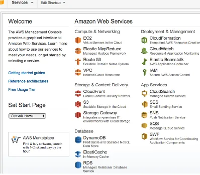
-‐ Signed in to Amazon Web Services Management Console, and clicked on
Figure 4.3: Amazon Web Services Management Console
-‐ Clicked “Launch Instance” from the Amazon EC2 Console Dashboard (figure
4.4):
Figure 4.4: Amazon EC2 Console Dashboard
-‐ When clicking on Launch Instance, a “Create a new instance” page was
[image:24.595.148.429.494.679.2]Figure4.5: Create a New Instance page
In this page, there were two ways to launch an instance:
• Classic Wizard, which offered more control and advance settings that
might be wanted.
• Quick Launch Wizard, which simplified the process to launch an
instance and also automatically configured many selections. In this project,
Classic Wizard was used, as it allowed the configuration of some specific
choices.
-‐ In the Quick Start tab, Microsoft Windows Server 2008 R2 Base was chosen
Figure 4.6: Choose the AMI from the Quick Start tap
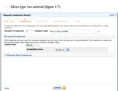
[image:26.595.88.504.350.670.2]-‐ Micro type was selected (figure 4.7):
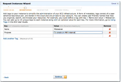
-‐ The name of the web server and a short description were entered (figure 4.8):
Figure 4.8: Naming the instance
[image:27.595.88.504.401.717.2]-‐ A key pair was created, securing the connection to the instance (figure 4.9):
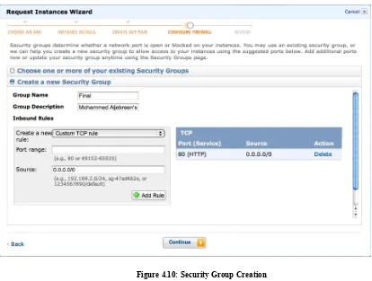
-‐ Then, a security group was created, defining the connection ports to the
[image:28.595.91.505.92.405.2]machine. 80 (HTTP) and 443 (HTTPS) ports were added (see figure 4.10):
Figure 4.10: Security Group Creation
-‐ The web server launched and took a few minutes to initialize (see figures 4.11,
4.12):
Figure 4.12: the web server started
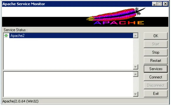
-‐ Apache web server, version 2.0.64 for Win32 platform was installed. The server’s
services included Apache web services (see figure 4.13):
[image:29.595.92.507.441.743.2]-‐ Here is the Apache Service Monitor screen (figure 4.14):
Figure 4.14: Apache Service Monitor
After launching a web server and installing all the needed services, a simple web site6
was designed, presenting services to the public. The page source code is:
<title>MOHAMMED ALJEBREEN</title>
<!DOCTYPE html PUBLIC "-//W3C//DTD XHTML 1.0 Transitional//EN" "http://www.w3.org/TR/xhtml1/DTD/xhtml1-transitional.dtd"> <html xmlns="http://www.w3.org/1999/xhtml">
<head>
<meta name="author" content="Wink Hosting (www.winkhosting.com)" /> <meta http-equiv="Content-Type" content="text/html; charset=iso-8859-1" />
<link rel="stylesheet" href="images/style.css" type="text/css" /> <title>Webserver</title>
</head> <body>
<div id="page" align="center">
<div id="content" style="width:800px"> <div id="logo">
<div style="margin-top:70px" class="whitetitle">R.I.T</div>
</div>
<div id="topheader">
<div align="left" class="bodytext"> <br />
<strong>Mohammed Aljebreen </strong><br /> 475 Countess Dr<br />
West Henrietta<br /> Phone: (585)309-3487<br /> [email protected]
</div>
<div id="toplinks" class="smallgraytext"> <a href="#">Home</a> | <a
href="#">Sitemap</a> | <a href="#">Contact Us</a> </div>
</div>
<div id="menu">
<div align="right" class="smallwhitetext" style="padding:9px;">
<a href="#">Home</a> | <a href="#">About Us</a> | <a href="#">Products</a> | <a href="#">Our Services</a> | <a href="#">Contact Us</a> </div> </div> <div id="contenttext"> <div style="padding:20px"> <span class="titletext">Final Project!</span> </div>
<div class="bodytext" style="padding:12px;" align="justify">
<strong>Hi! This is Mohammed Aljebreen. I'm going to present my final project which is about Implementing a Dynamic Scaling of Web Applications in a Virtualized Cloud Computing Environment.
</strong><br />
<br /> <br />
The committee members:<br /> Sharon Mason (chair)<br />
Lawrence Hill (committee memebr)<br /> Jim Leone (committee memebr)<br /> </div>
</div>
<span class="titletext">Permanently Server</span> <div style="padding:75px">
<div class="bodytext" style="padding:1px;" align="middle">
<strong>Here are three different galleries of pictures: </strong> <br />
</div>
<table align="center">
<tr>
<td><img src="images/animals.jpg" /></td> <td><img src="images/nature.jpg" /></td> <td><img src="images/plants.jpg" /></td> </tr>
<tr>
<td align="center"><a href="Photos.gz" target="_blank">Animals Pictures</a></td>
<td align="center"><a href="Photos1.gz" target="_blank">Nature Pictures</a></td>
<td align="center"><a href="Photos2.gz" target="_blank">Plants Pictures</a></td> </tr> </table> </div> <div style="padding:50px"> </div>
<div id="footer" class="smallgraytext">
<a href="#">Home</a> | <a href="#">About Us</a> | <a href="#">About RIT</a> | <a href="#">About NSSA</a> | <a href="#">Contact Us</a>
| aljebreen.org
-‐ The home web page of the website (see figure 4.15)
[image:32.595.92.508.71.461.2](http://loadbalancer.aljebreen.org):
Figure 4.15: The home page of the website
The purpose of this web page was to present services to the users. The website will be
used to test the proposed algorithm when applying a lot of load traffic to that website.
4.4.2 Creating an Amazon Machine Image (AMI):
What is the AMI? As defined by the Amazon Web Services website, “an Amazon
Machine Image (AMI) is a special type of pre-configured operating system and
virtual application software which is used to create a virtual machine within the
services delivered using EC2” [10]. It is like a template of a computer’s root volume
[11]. For example, an AMI could act as a web server or other data base server.
An AMI was created from the previously made instance in order to have an image of
the webserver that would be needed to scale up and down later when auto scaling
takes action.
-‐ The created AMI, named “clone”:
Figure4.16: The AMI from the web server
4.4.3 Creating an Amazon Load Balancer:
Amazon Elastic Load Balancing (see figure 4.17) consists of two elements: the load
balancer and the controller service. The purpose of the load balancer is to monitor the
traffic and handle the requests coming from the Internet. The purpose of the controller
service is to monitor the load balancer, verify its proper functioning, and add and
remove its capacity as needed.
The Elastic Load Balancing service on Amazon cloud will be used because it has
many useful features [12]:
● Distributing incoming traffic across Amazon EC2 instances.
● Automatically scaling the request in response to the incoming traffic.
● Creating and managing security groups to provide more networking and
security options when the Elastic Load Balancing is used in Virtual Private
● Detecting the health7 of the instances. Once an unhealthy load balance
instance has been detected, it will cease to route the traffic, and the rest of the
healthy instances will take care of routing instead.
Figure 4.17: Web server Load Balancer
[image:34.595.90.511.254.434.2]- Below, two servers are running under the load balancer (figure 4.18):
Figure 4.18: The servers under the load balancer
-‐ Webserver (1) and webserver (2) were added manually to the load balancer (see
figure 4.19); however, any new server will be added automatically.
Figure 4.19: Adding Webserver (1) & (2) to the Load Balancer
- In figure 4.20, HTTP is chosen as the ping protocol, and 80 as the ping port to
[image:35.595.120.494.97.331.2]allow the load balancer to receive incoming traffic.
Figure 4.20: Advanced Options of the load balancer’s configuration
• As the above figure shows, the configurations are set as follows:
Ping Protocol: HTTP
Ping Port: 80
Ping Path: /index.html
Response Timeout: 5 seconds, which is wait time before receiving a
response from the health check.
Health Check Interval: 0.5 minutes, which is the amount of time
between health check.
Unhealthy Threshold: 2 checks failures, which are the number of
health check failures before an EC2 instance is declared unhealthy.
Healthy Threshold: 10 succeed checks, which is the number of health
4.4.4 Configuring Amazon Auto Scaling:
The auto scaling was created using the CPU Utilization metric as an example.
The policies were set to:
Create a new temporary webserver when the CPU utilization of the
web server exceeded 80% for five minutes.
Remove the temporary webserver when the CPU utilization of web
server dropped less than 20% for five minutes.
Before creating an Auto Scaling, the proper command line tools must be
downloaded from the Amazon Web Services site. Java version 1.7 (see figure
4.21) must also be installed on the instance used to create auto scaling.
Figure 4.21: Java version 1.7 installed on the web server
-‐ The JAVA_HOME environment variable was set to point to Java installation
via this command:
C:\> set JAVA_HOME=C:\Program Files\Java\jre7
-‐ The %JAVA_HOME%\bin to %PATH environment variable was added:
C:\> set PATH=%PATH%;%JAVA_HOME%\bin
-‐ The AWS_AUTO_SCALING_HOME environment variable was set where the Auto
Scaling folder was unpacked:
C:\> set AWS_AUTO_SCALING_HOME=
C:\Users\Administrator\Desktop\AutoScaling-2011-01-01\AutoScaling-1.0.61.0
-‐ The %AWS_AUTO_SCALING_HOME%\bin to %PATH environment variable was
added:
-‐ The tools for the security credentials which were saved in a .template file were
configured. The file contained two security credentials: AWS access key ID,
and AWS secrete key.
C:\>set AWS_CREDENTIAL_FILE=C:\Users\Administrator\Desktop\
AutoScaling-2011-01-01\AutoScaling-1.0.61.0
-‐ The configuration was tested by using as-cmdcommand, and the resulting
[image:37.595.108.525.226.483.2]output (see figure 4.22), confirmed the installation:
Figure 4.22: Testing the Auto Scaling command line installation
- After testing the Auto Scaling installation and configuration, a launch config
(called MyAutoConfig), was created (see figure 4.23):
as-create-launch-config MyAutoConfig –image-id ami-1975da70 –
instance-type t1.micro –access-key-id AKIAIQS44P5ZBP244KQA –
secret-key KCvVpWgJ6cCnWOpOW3W3d+Ct4cSV3FnheGKBnDa3
--image-id: ami-1975da70
The AMI’s ID, which was created earlier, called Clone.
This is the type of instance that the image cloned from.
Amazon Elastic Compute instances (EC2) are grouped into
seven groups [13]: Standard, Micro, High-Memory, High-CPU,
Cluster Compute, Cluster GPU, and High I/O. Each type has
different characteristics that meet the user’s needs. The usage
charge is different from one group to another as well.
o Micro instances features:
• 613 MB memory
• Up to 2 EC2 Compute Units (for short periodic bursts)
• EBS storage only
• 32-bit or 64-bit platform ( I chose 64-bit)
• I/O Performance: Low
• API name: t1.micro
--access-key-id & --secret-key: these are the credential security keys.
Figure 4.23: MyAutoConfig creation
- An Auto Scaling group was then created and named MyGroup2 (see figure 4.24):
as-create-auto-scaling-group MyGroup2 –launch-configuration
MyAutoConfig –availability-zones us-east-1a –min-size 1 –max-size
4 –load-balancers Webserver-Load-Balancer –access-key-id
AKIAIQS44P5ZBP244KQA –secret-key
■ –launch-configuration: MyAutoConfig , which is the name of the launch
configuration that was previously created.
■ –availability-zones: us-east-1a , defines which zone that the instances
will be launched.
o Amazon has seven different physical locations that can be used
to launch instances conveniently and be closer to your
costumers. For the experiment, the Northern Virginia region
was chosen, as it was the closest region to Rochester, NY. The
seven regions are [14]:
US East (Northern Virginia) Region
US West (Northern California) Region
US West (Oregon) Region
EU (Ireland) Region
Asia Pacific (Singapore) Region
Asia Pacific (Tokyo) Region
South America (Sao Paulo) Region
■ –min-size 1: the minimum number of instances that the Auto Scaling
will not lower.
■ –max-size 4: the maximum number of instances that the Auto Scaling
will not exceeded.
■ --load-balancers :Webserver-Load-Balancer, the name of the load balancer
that was created. All new instances will belong to it.
Figure 4.24: MyGroup2 creation
- Verifying the Auto Scaling Group creation as in figure 4.25:
as-describe-auto-scaling-groups –headers –access-key-id
AKIAIQS44P5ZBP244KQA –secret-key
KCvVpWgJ6cCnWOpOW3W3d+Ct4cSV3FnheGKBnDa3
Figure4.25: Verifying the Auto Scaling Group creation
- Also, verifying the Auto Scaling instances, which has only one instance (see
figure 4.26):
as-describe-auto-scaling-instances –headers –access-key-id
AKIAIQS44P5ZBP244KQA –secret-key
KCvVpWgJ6cCnWOpOW3W3d+Ct4cSV3FnheGKBnDa3
- The first scale up policy created was named ScaleUpPolicy (see figure 4.27):
as-put-scaling-policy ScaleUpPolicy –auto-scaling-group MyGroup2 –
adjustment=1 –type ChangeInCapacity –cooldown 60 –access-key-id
AKIAIQS44P5ZBP244KQA –secret-key
KCvVpWgJ6cCnWOpOW3W3d+Ct4cSV3FnheGKBnDa3
--auto-scaling-group: MyGroup2 , the Auto Scaling group.
--adjustment=1: adds one instance when the CPU utilization reaches its
defined upper level.
--type ChangeInCapacity: This option was chosen because it could adjust
by constant increment. The alternative option was
“PercentChangeInCapacity”, which adjusts by the percentage of the current
capacity.
--cooldown 60 seconds: the period that helps prevent the Auto Scaling
from initiating more activities before the previous activities are visible.
Figure 4.27: Scale Up Policy
This command generates an ARN, which represents the action of the scaling up
policy. This policy would use ARN to associate Auto Scaling policies with
CloudWatch alarms for scaling up, which will be explained later:
arn:aws:autoscaling:us-east-1:131511199887:scalingPolicy:b8d78a4a-04a5-4f9b-b175-c26ce7aa1569:autoScalingGroupName/
MyGroup2:policyName/ScaleUpPolicy
- A second policy, this time to scale down, was created and named
as-put-scaling-policy ScaleDownPolicy –auto-scaling-group MyGroup2 “–
adjustment=-1” –type ChangeInCapacity –cooldown 300 –access-key-id
AKIAIQS44P5ZBP244KQA –secret-key
KCvVpWgJ6cCnWOpOW3W3d+Ct4cSV3FnheGKBnDa3
All these parameters are explained in the previous step.
--adjustment=-1: deletes one instance when the CPU utilization
reaches its defined lower level.
Figure 4.28: Scale Down Policy
In this step, the ARN action associated the policy with CloudWatch alarms for scaling
down:
arn:aws:autoscaling:us-east-1:131511199887:scalingPolicy:d215e8d8-b5d3-4825-a5a5-a9622c9fb10e:autoScalingGroupName/MyGroup2:
policyName/ScaleDownPolicy
4.4.5 Creating CloudWatch Alarms:
The Cloud Watch Alarms were created to notify when any of the Auto Scaling actions
were taking place. The cloud watch alarms were set to follow the main server, and
when the CPU utilization reaches any of the triggers that were set for the Auto
Scaling, it takes action accordingly. In addition, the alarm sends a notification email
each time.
To create the CloudWatch alarms, its command line tools must be installed. The
environment for the command line was set as follows:
-‐ The AWS_CLOUDWATCH_HOME environment variable was set where the
C:\> set AWS_AUTO_SCALING_HOME= C:\Users\Administrator\Desktop\
CloudWatch-2010-08-01\CloudWatch-1.0.12.1
-‐ The %AWS_AUTO_SCALING_HOME%\bin to %PATH environment variable was
added:
C:\> set PATH=%PATH%;%AWS_COULDWATCH_HOME%\bin
-‐ The tools for security credentials were configured and saved in a .template
file. The file contains two security credentials: AWS access key ID, and AWS
secrete key.
Set AWS_CREDENTIAL_FILE=C:\>set AWS_CREDENTIAL_FILE=C:\Users\
Administrator\Desktop\CloudWatch-2010-08-01\CloudWatch-1.0.12.1
- The configurations were tested by using a mon-cmd command, and the
[image:43.595.110.523.345.547.2]resulting output (see figure 4.29) confirmed the installation:
Figure 4.29:Testing the CloudWatch command line installation
-‐ The first alarm created was called “HighCPU-alarm” (see figure 4.30). Once
the CPU reaches its defined high level (>= 80), the alarm runs the ARN policy
action and sends a notification when the Auto Scaling creates a new web
server instance:
mon-put-metric-alarm HighCPUAlarm --comparison-operator
CPUUtilization --namespace "AWS/EC2" --period 300 --statistic
Average --threshold 80 --alarm-actions
arn:aws:autoscaling:us-east-
1:131511199887:scalingPolicy:b8d78a4a04a54f9bb175c26ce7aa1569:autoScalingGroupName/MyGroup2:policyName/ScaleUpPolicy
--dimensions "AutoScalingGroupName=MyGroup2" --access-key-id
AKIAIQS44P5ZBP244KQA --secret-key
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
--comparison-operator GreaterThanThreshold: the operator used to scale up, in
this case, the GreaterThanThreshold.
--evaluation-periods 1: Number of consecutive periods for which the value of
the metric needs to be compared to the threshold [15].
--metric-name CPUUtilization: The metric used.
--namespace"AWS/EC2": the name space for the alarms. Here, it is the default
name.
--period 300: after 300 seconds, the metric would set off the alarm.
--statistic Average: The average between periods. The minimum or the maximum can also be used.
--threshold 80: The alarm would take place when the CPU utilization reaches
80%.
--alarm-actions arn:aws:autoscaling:us-east-1:131511199887:scalingPolicy:b8d78a4a-04a5-4f9b-b175-c26ce7aa1569:autoScalingGroupName/MyGroup2:policyName/
ScaleUpPolicy: The connection between the alarm action and the Auto Scaling.
--dimensions "AutoScalingGroupName=MyGroup2": all available instances were
filtered by the name of the group for Auto Scaling: MyGroup2.
Figure 4.30: HighCPU-alarm
-‐ The second alarm created was called “LowCPU-Alarm” (see figure 4.31).
Once the CPU reaches its defined low level (<= 20), the alarm runs the ARN
policy action and sends a notification when the Auto Scaling deletes an
instance:
mon-put-metric-alarm LowCPUAlarm --comparison-operator
LessThanThreshold --evaluation-periods 1 --metric-name
CPUUtilization --namespace "AWS/EC2" --period 300 --statistic
Average --threshold 20 --alarm-actions
arn:aws:autoscaling:us-east-
1:131511199887:scalingPolicy:d215e8d8-b5d3-4825-a5a5-a9622c9fb10e:autoScalingGroupName/MyGroup2:policyName/ScaleDownPolicy
--dimensions "AutoScalingGroupName=MyFirstGroup" --access-key-id
AKIAIQS44P5ZBP244KQA --secret-key
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
All the parameters were explained in the previous step. In the --comparison-operator the LessThanThreshold was used as an operator to scale down.
[image:45.595.94.510.594.695.2]-‐ The alarms of the CloudWatch in AWS management console (see figure 4.32):
Figure 4.32: The alarms of the CloudWatch in AWS management console
5. DEMONSTRATIONS &RESULTS:
5.1Auto Scaling Testing:
After testing the Auto Scaling policies for scaling up and scaling down, they worked
perfectly. The Wget tool was used to download the entire website content using three
different shells. As a result, the Auto Scaling created a new web server:
Figure 5.1: Auto Scaling creates an instance
As shown under “Status Checks” in Figure 5.1, the new instance was initializing. It
took about two minutes until it was ready to use.
The testing of the creation of the new instance showed that scaling up features
worked. To test the scaling down features, the newly created instance was deleted
when the CPU utilization reached its lower level. The download was halted from the
webserver (1) and, as a result, the CPU utilization became less than 20% for five
Figure5.2: CloudWatch Alarms8
-‐ The alarm sent a notification email:
Figure 5.3: A notification email in [email protected] inbox
8 As it appears, the LowCPU-alarm is reached its goal, which means that the CPU utilization in that moment became less that 20% for two minutes, which allowed the Auto Scaling to remove the temporary web server. The HighCPU-Alarm is still in its range, which means the CPU utilization was still fewer than 80%, so I can see the green sign next to the alarm.
- After the CPU utilization became less than 20% for five minutes, the
ScalingDown policy took place and shut the temporary instance down (figure
5.4):
Figure 5.4: shutting the temporary instance down
- The instance was then terminated (see figure 5.5):
Figure 5.5: Terminating the temporary instance
- Afterwards, the experiment was successfully scaled up and down of the proposed
algorithm (see figure 5.4).
5.2Tests’ Results:
In these next tests, the auto scaling actions did not take place. The reason was
to monitor the web server’s performance during the tests without scaling up (adding a
new instance) or scaling down (deleting an instance), which would help decide which
metric is the best overall. To clarify this point, let’s take this example: perhaps the
auto scaling action would take place during the test time, and the CPU Utilization
exceeded the high boundary (which was 80%) only for five minutes and returned back
to 60% for the rest of the test period. The auto scaling would create a new instance
because it exceeded 80% for 5 minutes, and it would not delete it because it did not
exceed the low boundary (20%), thus preventing the web server from exceeding the
upper boundary alone without additional instances. However, placing an alarm action,
instead of auto scaling action is more beneficial to the experiment as it is
non-intrusive.
After testing, the results were analyzed using tables and graphs, as shown
below:
5.2.1 CPU Utilization Metric Results:
5.2.1.1First Test:
Test Place High Alarm Period (~ minutes) (>=80 %)
Low Alarm Period (~minutes) (<=20%)
Morning
Weekdays RIT 0 0
Evening
Weekdays RIT 12 4
Morning
Weekends RIT 25 0
Evening
Weekends RIT 17 2
Morning
Weekdays Home 10 8
Evening
Weekdays Home 0 19
Morning
Weekends Home 0 22
Evening
Weekends Home 0 27
Virginia 30 0
Oregon 8 12
[image:49.595.87.521.646.739.2]North California 2 6
Table 2: CPU Utilization Metric Results of the First Test
o Weekday evenings at RIT System Lab
o Weekend mornings at RIT System Lab
o Weekend evenings at RIT System Lab
o Weekday evenings from home
o Weekend mornings from home
o Weekend evenings from home
o From a server within Amazon cloud in the same geographic region,
o From a server within Amazon cloud in Oregon geographic region
o From a server within Amazon cloud in Northern California geographic
region
5.2.1.2Second Test:
CPU Utilization in the second test was always around 4% for most of the tests, even
when the server was receiving around 45 connections per minute.
Test Place High Alarm Period (~ minutes) (>=80 %)
Low Alarm Period (~minutes) (<=20%)
Morning
Weekdays RIT 0 During the whole test period Evening
Weekdays RIT 0 During the whole test period Morning
Weekends RIT 0 During the whole test period Evening
Weekends RIT 0 During the whole test period Morning
Weekdays Home 0 During the whole test period Evening
Weekdays Home 0 During the whole test period Morning
Weekends Home 0 During the whole test period
Weekends Home
Virginia 9 Only 2 minutes above 20%
Oregon 0 During the whole test period
[image:53.595.86.569.42.109.2]North California 0 During the whole test period
Table 3: CPU Utilization Metric Results of Second Test
o Weekday mornings at RIT System Lab
o Weekday evenings at RIT System Lab
o Weekend evenings at RIT System Lab
o Weekday mornings from home
o Weekday evenings from home
o Weekend evenings from home
In this test, the performance jumped to 30% for 25 minutes. Although this
is an outlier result, it was still taken into consideration.
o From a server within Amazon cloud in the same geographic region,
Virginia web server
o From a server within Amazon cloud in Northern California geographic
region
5.2.2 Network Out Metric Results:
5.2.2.1First Test:
Test Place High Alarm Period (~ Minutes) (>= 2 GB)
Low Alarm Period (~ Minutes) (<= 5 MB) Morning
Weekdays RIT 34 0
Evening
Weekdays RIT 25 2
Morning
Weekends RIT 35 0
Evening
Weekends RIT 32 2
Morning
Weekdays Home 9 4
Evening
Weekdays Home 0 19
Morning
Weekends Home 0 22
Evening
Weekends Home 0 31
Virginia 35 0
Oregon 9 13
[image:56.595.90.523.110.181.2]North California 3 6
o Weekday mornings at RIT System Lab
o Weekday evenings at RIT System Lab
o Weekend mornings at RIT System Lab
o Weekday mornings from home
o Weekday evenings from home
o Weekend mornings from home
o From a server within Amazon cloud in the same geographic region,
Virginia web server
o From a server within Amazon cloud in Oregon geographic region
o From a server within Amazon cloud in Northern California geographic
region
5.2.2.2Second Test:
Test Place High Alarm Period (~ Minutes) (>= 2 GB)
Low Alarm Period (~ Minutes) (<= 5 MB) Morning
Weekdays RIT 0 During the whole test period Evening
Weekdays RIT 0 During the whole test period Morning
Weekends RIT 0 During the whole test period Evening
Morning
Weekdays Home 0 During the whole test period Evening
Weekdays Home 0 During the whole test period Morning
Weekends Home 0 During the whole test period Evening
Weekends Home 0 During the whole test period
Virginia 0 During the whole test period
Oregon 0 During the whole test period
[image:60.595.84.550.42.221.2]North California 0 During the whole test period
Table 5: Network Out Metric Results of Second Test
o Weekday mornings at RIT System Lab
o Weekend mornings at RIT System Lab
o Weekend evenings at RIT System Lab
o Weekday mornings from home
o Weekend mornings from home
o Weekend evenings from home
o From a server within Amazon cloud in the same geographic region,
Virginia web server
o From a server within Amazon cloud in Northern California geographic
region
5.2.3 Latency Metric Results:
5.2.3.1First Test:
Test Place High Alarm Period
(~ Minutes) (.30 Second)
Low Alarm Period (~ Minutes) (<= .005 Second) Morning
Weekdays RIT 9 0
Evening
Weekdays RIT 2 27
Morning
Weekends RIT 0 25
Evening Weekends RIT
During the whole test period except 4
minutes 0
Morning
Weekdays Home 5 0
Evening
Weekdays Home 0 0
Morning
Weekends Home 8 8
Evening
Weekends Home 1 0
Virginia 13 0
Oregon 0 0
[image:63.595.92.524.114.183.2]North California 0 0
o Weekday mornings at RIT System Lab
o Weekday evenings at RIT System Lab
o Weekend mornings at RIT System Lab
o Weekday mornings from home
o Weekday evenings from home
o Weekend mornings from home
o From a server within Amazon cloud in the same geographic region,
Virginia web server
o From a server within Amazon cloud in Oregon geographic region
o From a server within Amazon cloud in Northern California geographic
region
5.2.3.2Second Test:
Test Place High Alarm Period
(~ Minutes) (>.30 Second)
Low Alarm Period (~ Minutes) (<= .005 Second) Morning
Weekdays RIT 6 0
Evening
Weekdays RIT 5 0
Morning
Weekends RIT 43 0
Evening
Morning
Weekdays Home 18 0
Evening
Weekdays Home 47 0
Morning
Weekends Home 53 0
Evening
Weekends Home 46 0
Virginia 53 0
Oregon 57 0
[image:67.595.87.577.42.221.2]North California 17 0
Table 7: Latency Metric Results of First Test
o Weekday mornings at RIT System Lab
o Weekday evenings at RIT System Lab
o Weekend evenings at RIT System Lab
o Weekday mornings from home
o Weekday evenings from home
o Weekend evenings from home
o From a server within Amazon cloud in the same geographic region,
Virginia web server
o From a server within Amazon cloud in Northern California geographic
region
5.2.4 Request Counts Metric Results:
5.2.4.1First Test:
Test Place High Alarm Period
(~ Minutes) (>= 200 Counts)
Low Alarm Period (~ Minutes) (<2 Counts) Morning
Weekdays RIT 0 19
Evening
Weekdays RIT 0 18
Morning
Weekends RIT 0 34
Evening
Weekends RIT 0 27
Morning
Weekdays Home 0 35
Evening
Weekdays Home 0 During the whole test period Morning
Weekends Home 0 During the whole test period Evening
Weekends Home 0 During the whole test period
Virginia 0 27
Oregon 0 34
[image:70.595.91.521.112.192.2]North California 0 31
o Weekday mornings at RIT System Lab
o Weekday evenings at RIT System Lab
o Weekend mornings at RIT System Lab
o Weekday mornings from home
o Weekday evenings from home
o Weekend mornings from home
![Figure 1.1: Typical Cloud Computing Environment [2]](https://thumb-us.123doks.com/thumbv2/123dok_us/43067.3898/13.595.134.461.47.306/figure-typical-cloud-computing-environment.webp)
![Figure 4.2: Architecture to Scale Web Applications in a Cloud [1]](https://thumb-us.123doks.com/thumbv2/123dok_us/43067.3898/23.595.156.457.220.444/figure-architecture-scale-web-applications-cloud.webp)