TECHNOLOGIES UNDER RISK: A STUDY OF
SMALL UPLAND FARMS IN BATANGAS, PH ILIPPINES
by
Constancia G. Maranan, B.Sc. Agri.
A Dissertation submitted in partial fulfillment of the requirements for the Degree of
Master of Agricultural Development Economics in the Australian National
DECLARATION
Except where otherwise indicated, this
dissertation is my own work.
lUü M aK&nan
Constancia G. Maranan
July 1983
•*•**■** •*1•t f i r\
' b
%
ACKNOWLEDGEMENTS
I wish to express my gratitude to the Development Studies Centre, for granting me the DSC fellowship which enabled me to study at the Australian National Lniversity.
I am very much indebted to my supervisor , Dr Colin Barlow for all his help and guidance. Also, Dr Sisira Jayasuriya who supervised the latter stages of this thesis. His valuable suggestions and criticisms have helped to put this thesis in final form. To both of them, I owe a lot for which words can not express my deep gratitude.
I am also grateful to the following people: Dr Edwin Price of the IRRI who had provided me access to use the data needed in this study; Dr Tony Oakwell of the Bureau of Agricultural Economics, Canberra, for his help in sorting some problems in the model used at the earlier stages of this study; Mr Peter Oates for helping me with my computer problems; Mr Chris Blunt for all his assistance in the preparation of this manuscript; Mr Nelson Genito and Gerry Erguiza in the preparation of graphs and figures; to the M.A.D.E. staff for information and suggestions; also, to Ms Norma Chin for her excellent typing.
ABSTRACT
Risk is considered to be one of the factors that affects farmers'
use of new agricultural technology. This study uses a mathematical
programming technique which takes into account both
income and risk considerations in evaluating some new technologies
developed for small upland farmers in the Philippines. The possible
impact of introducing new rice and sorghum varieties is investigated
through the model. The results show that those models with both
income and risk considerations with an additional priority of meeting
the subsistence requirements for rice simulate actual farm decision
making better than those not incorporating risk and such an objective.
The results suggest that a new rice variety will replace the
traditional variety, even where it gives only a 25% additional yield.
Also, the new rice technology is likely to be adopted by farmers
irrespective of the degree of their risk aversion. On the other hand
sorghum is adopted widely only where its price or yield is twice the
existing level, although risk is not again increased. Further, given
additional land of any type (either owned or share tenanted) farmers
are likely at existing price and yields to plant a larger area of both
a new rice variety and sorghum. Moreover, the increase in available
family labour per household has little effect on the adoption of both
new rice and sorghum technologies.
While results are indicative of the potential of the new
technologies, there are methodological and estimational problems in
applying the MOTAD approach in assessing the impact of the
introduction of new technologies. These would have to be considered
CONTENTS
DECLARATION ii
ACKNOWLEDGEMENTS iii
ABSTRACT iv
LIST OF TABLES vii
LIST OF FIGURES ix
LIST OF APPENDICES xii
CHAPTER 1. INTRODUCTION 1
1.1 Objectives of the Study 3
1.2 Outline of the Thesis 3
CHAPTER 2. BACKGROUND TO THE STUDY 5
2.1 Description of the Batangas Research Site 5
2.2 Farm Characteristics and Cropping Patterns 10
2.3 Level of Resources Used 13
2.4 Yield and Output Prices 14
CHAPTER 3. DECISION-MAKING UNDER RISK 20
3.1 Concept of Risk and Uncertainty 20
3.2 Sources of Risk in Agricultural Production 21
3.2.1 Yield risk 21
3.2.2 Price risk 22
3.3 Criteria for Risky Decision-Making 22
3.3.1 Expected profit maximization 23
3.3.2 Expected utility maximization 23
3.3.3 Safety first rules of thumb 26
3.4 Widely Used Approaches for Accounting for
Risk in Farm Decision-Making 27
3.4.1 Mean variance approach 27
3.4.2 Stochastic dominance rule 30
CHAPTER 4. METHODOLOGY 35
4.1 Rationale for the Choice of the Model 35
4.2 The Model 36
4.2.1 Deterministic linear programming
(LP non-risk) model 36
4.2.2 Minimization of total absolute deviation
(MOTAD) model 37
4.3 Application of Similar Models in Other Studies 40
4.4 The Assumptions of the MOTAD Model 45
4.5 Data Used in the Study 46
4.5.1 Description of the sample farmers 46
4.5.2 The average farm model 47
4.6 Evaluation of Technologies 51
CHAPTER 5. EMPIRICAL RESULTS 54
5.1 Farmers Existing Technologies’ 54
5.2 Impact of the Introduction of New Technologies 60
5.2.1 Existing + available new technologies 60
5.2.2 Existing + available + potential new
technologies 65
CHAPTER 6. EFFECTS OF CHANGES IN RESOURCE ENDOWMENTS, PRICE AND YIELD LEVELS IN THE CHOICE OF
TECHNOLOGIES, FARM INCOME AND RISK 71
6.1 Labour Supply 71
6.2 Land Supply 73
6.3 Changes in Price and Yields of New Rice Variety
and Sorghum 83
6.3.1 Changes in price 83
6.3.2 Changes in yield 86
CHAPTER 7. SUMMARY, CONCLUSIONS AND IMPLICATIONS 94
BIBLIOGRAPHY 100
LIST OF TABLES
Table Title
2.1 Area and production of upland rice in the
Philippines, by region, 1973 6
2.2 Baseline information of 35 co-operating farmers,
Cale, Tanauan, Batangas, 1973 11
2.3 Percentage of land planted to various cropping
patterns, 35 farms, Cale, Tanauan, Batangas,
1973-77 12
2.4 Total cropped area, farm size and multiple
cropping index, 35 farmers, Cale, Tanauan,
Batangas, 1973-77 13
2.5 Changes in the allocation of inputs by crop/crop
group, 35 farmers, Cale, Tanauan, Batangas,
1973-77 15
2.6 Changes in yield of different crop/crop groups,
35 farms, Cale, Tanauan, Batangas, 1973-77 17
4.1 Outline of the linear programming (non-risk) matrix 41
4.2 Outline of the linear risk programming matrix 42
4.3 General information on five selected farms, Cale,
Tanauan, Batangas, 1977 47
4.4 Percentage of land planted to various cropping
patterns, 5 selected farms, Cale, Tanauan,
Batangas, 1974-77 48
4.5 Resource constraints assumed for the average
farm assumed in the model 51
5.1 Optimal farm plan estimated from the LP
deterministic model, existing technologies 55
5.2 Optimal farm plans estimated from the MOTAD
model, existing technologies 57
5.3 Optimal farm plan estimated from the LP
deterministic model, existing + available new
technologies 62
5.4 Optimal farm plans estimated from the MOTAD model,
existing + available new technologies 66
5.5 Optimal farm plans estimated from the MOTAD model,
existing + available + potential new
LIST OF FIGURES
Figure Title
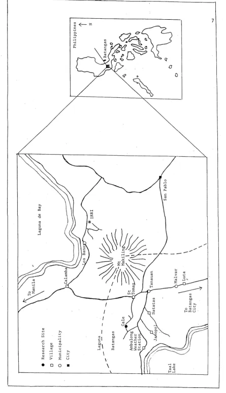
2.1 Location of cropping systems research site in
Batangas Province, Philippines
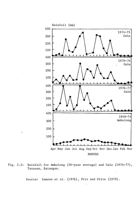
2.2 Rainfall for Ambulong (26-year average) and Cale
(1974-77), Tanauan, Batangas
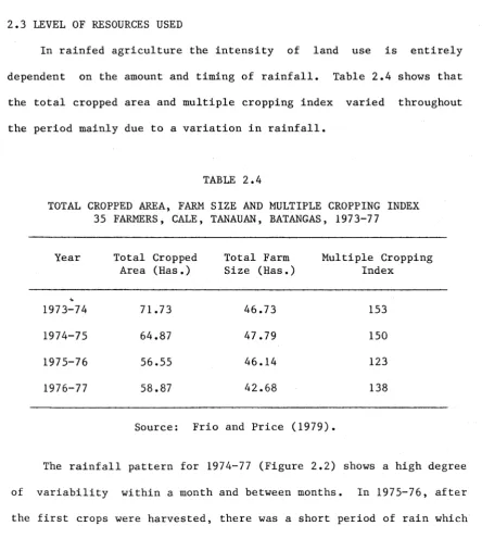
2.3 Percentage of total manhours for various crop
operations spent on each crop, Cale, Tanauan, Batangas, 1973-77
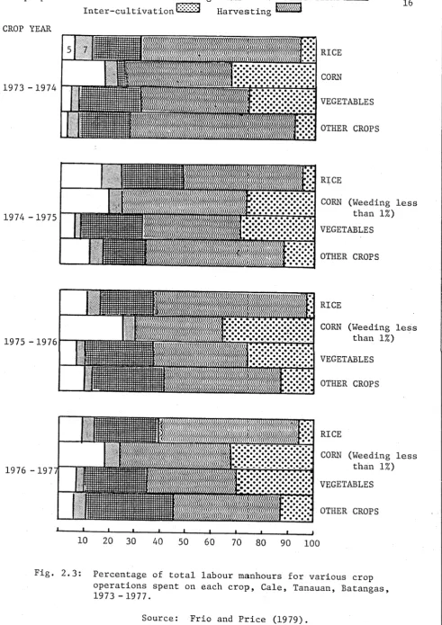
2.4 Quarterly prices of selected crops, Divisoria
Market, Manila
3.1 Three possible shapes of utility functions for
three individuals
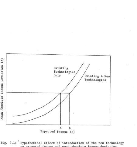
4.1 Hypothetical effect of introduction of new
technology on expected income and mean absolute income deviation
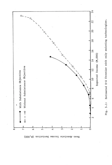
5.1 Estimated E-A frontier with existing technologies
5.2 Estimated E-A frontier with introduction of new
technology, existing + available new technologies
5.3 Estimated E-A frontier with introduction of new
technology, existing + available + potential new technologies
6.1 Effects of increases in family labour on expected
income and mean absolute income deviation, existing technologies, with subsistence objective
6.2 Effects of increases in family labour on
percentage of total area planted to NT, expected income and mean absolute income deviation, existing + available new technologies, with subsistence objective
6.3 Effects of increases in family labour on
percentage of total area planted to NT, expected income and mean absolute income deviation, existing + available + potential new technologies, with subsistence objective
52
59
72
74
6.4
6.5
6.6
6.7
6.8
6.9
6 . 1 0
6 . 1 1
6 . 1 2
Effects of increases in area of fully owned land on percentage of total area planted to
traditional rice, expected income and mean absolute income deviation, existing
technologies, with subsistence objective 76
Effects of increases in area of fully owned land on percentage of total area planted to NT, expected income and mean absolute income deviation, existing + available new
technologies, with subsistence objective 78
Effects of increases in area of fully owned land on percentage of total area planted to NT, expected income and mean absolute income deviation, existing + available + potential
new technologies, with subsistence objective 79
Effects of increases in area of share tenanted land (3:1) on expected income and mean absolute income, existing technologies,
with subsistence objective 80
Effects of increases in area of share tenanted land (3:1) on percentage of total area planted to NT, expected income and mean absolute income deviation, existing +
available new technologies, with subsistence
objective 81
Effects of increases in area of share tenanted land (3:1) on percentage of total area planted to NT, expected income and mean absolute income deviation, existing +
available + potential new technologies, with
subsistence objective 82
Effects of increases in price of rice on percentage of total area planted to NT, expected income and mean absolute income deviation, existing + available new
technologies, with subsistence objective 84
Effects of changes in price of rice on percentage of total area planted to NT, expected income and mean absolute income deviation, existing + available + potential new technologies,
with subsistence objective 85
Effects of changes in price of sorghum on percentage of total area planted to NT, expected income and mean absolute income deviation, existing + available + potential
6.13 Effects of changes in price of rice and sorghum on percentage of total area planted to NT, expected income and mean absolute income deviation, existing + available + potential
new technologies, with subsistence objective 88
6.14 Effects of changes in yield of rice on percentage
of total area planted to NT, expected income and mean absolute income deviation, existing + available + potential new technologies,
with subsistence objective 89
6.15 Effects of changes in yield of rice on percentage
of total area planted to NT, expected income and mean absolute income deviation, existing + available new technologies, with subsistence
objective 90
6.16 Effects of changes in yield of sorghum on
percentage of total area planted to NT, expected income and mean absolute income deviation, existing + available + potential
new technologies, with subsistence objective 91
6.17 Effects of changes in yield of rice and sorghum on
percentage of total area planted to NT, expected income and mean absolute income deviation, existing + available + potential
LIST OF APPENDICES
Table Title
A. 1 Crop production vectors included in the model 106
B.l Prices of output used in the model 107
B.2 Prices of input used in the model 108
C.l Crop combinations along the E-A frontier with
increases in family labour, existing
technologies, with subsistence objective 109
C. 2 Crop combinations along the E-A frontier with
increases in family labour, existing + available new technologies, with
subsistence objective 110
C.3 Crop combinations along the E-A frontier with
increases in family labour, existing + available + potential new technologies,
with subsistence objective 111
D.l Crop combinations along the E-A frontier with
increases in area of fully owned land, existing technologies, with subsistence
obj ective 112
D . 2 Crop combinations along the E-A frontier with
increases in area of fully owned land, existing + available new technologies,
with subsistence objective 113
D.3 Crop combinations along the E-A frontier with
increases in area of fully owned land, existing + available + potential new
technologies, with subsistence objective 114
E.l Crop combinations along the E-A frontier with
increases in area of share tenanted land, existing technologies, with subsistence
objective 115
E . 2 Crop combinations along the E-A frontier with
increases in area of share tenanted land, existing + available new technologies, with
subsistence objective 116
E . 3 Crop combinations along the E-A frontier with
increases in area of share tenanted land, existing + available + potential new
F.l
F . 2
F.3
G. 1
G. 2
H.l
1.1
J.l
J . 2
K. 1
L. 1
Crop combinations along the E -A frontier with increases in area of all land t y p e s , existing technologies, with subsistence obj ective
Crop combinations along the E -A frontier with increases in area of all land t y p e s ,
existing + available new technologies, with subsistence objective
Crop combinations along the E-A frontier with increases in area of all land t y p e s , existing + available + potential new technologies, with subsistence objective
Crop combinations along the E- A frontier with increases in price of rice, existing +
available new technologies, with subsistence obj ective
Crop conbinations along the E -A frontier with increases in price of rice, existing + available + potential new tech n o l o g i e s , with subsistence objective
Crop combinations along the E - A frontier with increases in price of sorghum, existing + available + potential new technologies, with subsistence objective
Crop combinations along the E- A frontier with increases in price of rice and sorghum, existing + available + potential new technologies, with subsistence objective
Crop combinations along the E - A frontier with increases in yield of rice, existing +
available new technologies, with subsistence objective
Crop combinations along the E-A frontier with increases in yield of rice, existing + available + potential new technologies, with subsistence objective
Crop combinations along the E-A frontier with increases in yield of sorghum, existing + available + potential new technologies, with subsistence objective
Crop combinations along the E-A frontier with increases in yield of rice and sorghum, existing + available + potential new technologies, with subsistence objective
118
119
120
121
122
123
124
125
126
127
Figure A. 1
B . l
C.
l
LIST OF APPENDICES
Title
Effects of increases in all land types on percentage of total area planted to
traditional rice, expected income and mean absolute income deviation, existing
technologies, with subsistence objective Effects of increases in all land types on
percentage of total area planted to NT, expected income and mean absolute income deviation, existing + available new technologies, with subsistence objective Effects of increases in all land types on
percentage of total area planted to NT, expected income and mean absolute income deviation, existing 4- available + potential new technologies, with subsistence objective
129
130
In the Philippines, agriculture plays a major part in the
economy. It provides employment for two-thirds of the population and
contributes about one-third of the national income. Because of this,
its development is very vital. Development in agriculture can be
achieved in many ways. The introduction of new agricultural
technology is considered to be an important way of developing this
sector.
In the last two decades, many agricultural institutions have been
involved in developing and introducing new technologies to increase
the productivity and income of many small farmers in less developed
countries. Despite this, the problems of low productivity and
consequently low income among farmers continues. This is because the
farmers' use of new technologies has not been as widespread as
expected. Recognizing this problem, many agricultural scientists
believe that a new technology would gain wider acceptance if it were
evaluated and modified at various stages of its generation.
Evaluation can either be done at the design stage (ex-ante) or after
field testing (ex-post). In the International Rice Research Institute
(IRRI) cropping systems program, ex-post evaluation of new
technologies is widely practiced. However, ex-ante evaluation might
be appropriate with a cropping systems research. Barlow (1979) had
of new technologies fitted to specific farming circumstances; (b)
avoidance of introducing inappropriate technology for large-scale
programs and consequently minimizing cost of failure if it should take
place.
The most common method of evaluating the benefits of new
technologies is through a costs and returns analysis. The advantage
of using this method is that it can easily assess the likely benefits
of new technology over traditional technology without the need for
sophisticated calculations. The major disadvantage is that, being a
partial analysis, it only gives the return above the variable cost of
production and does not give an indication whether a new technology is
feasible and fitted to the farmers' total available resources.
An alternative method is the whole farm approach via linear
programming. Such an approach was used by Barlow et a l . (1979) and
Labadan et al. (1980) in the evaluation of cropping systems
technologies developed for small farmers in the Philippines. Although
their study gave results superior to those obtained with a costs and
returns analysis, the risks associated with the introduced
technologies were completely ignored. The high level of risk
associated with new technology is considered to be one of the critical
factors that limits its adoption, especially by small farmers whose
production resources are low. In this regard, an evaluation approach
which takes into account not only the resource constraints but also
the risk associated with the new technology is desirable. Through
this approach, the degree of acceptability of the new technology to
the farmers in the specific localities for which they are designed,
1.1 OBJECTIVES OF THE STUDY
The aim of this study is to evaluate some new technologies
developed for upland farms in the Batangas province in the Philippines
where risk is considered important. Data are obtained from the IRRI’s
cropping systems program gathered from a group of farmers growing a
multiplicity of crops. The economic benefits of new cropping systems
technologies are evaluated by the use of the Minimization of Total
Absolute Deviation (MOTAD) approach developed by Hazell (1971). In
this approach both income and risk considerations are incorporated in
the evaluation procedure.
Specifically, the objectives are:
(i) to analyze the choice of technologies by selected farms with
different resource endowments, and to examine how their choice
is affected by risk.
(ii) to evaluate the farm level impact of the introduction of a
number of new technologies (some of which are already available,
and others which are currently being developed) having different
input requirements, returns and degree of risk.
(iii) to assess the implications of results obtained on the potential
of the new technologies for large-scale farm level adoption and
the consequence of such adoption on farm income.
1.2 OUTLINE OF THE THESIS
In Chapter 2, background information is given on the IRRI
research site in Batangas, Philippines. The farming system operated
by farmers is described in detail.
In Chapter 3, decision-making under risk is discussed.
risky decision-making and in the last section some approaches for accounting for risk in models of farm decision-making.
In Chapter 4, the methodology adopted is presented. The models used are discussed. Included also in the discussion are the review of studies where a similar model is used. The major assumptions of the model used are also given. In the later part, the data used in the study are presented. The crop and non-crop activities considered in the construction of the programming matrix are discussed. Lastly, the procedure used in the assessment of the potential of the new technologies are presented.
In Chapter 5, results from the model using the average farm model are presented. In the first part, the results from the model with only the existing technologies are presented. In the second part, the impact of the introduction of the new technologies are analyzed. In the first case, only the new rice variety was included in the existing model and in the second case, both the new rice variety and sorghum are included in the model. In all cases, the model results from the LP deterministic and MOTAD models with and without the consumption objective are discussed.
In Chapter 6, results are presented on how differences in the resource endowments of the sample farms would affect the acceptance of the new technology. This is done by parametrizing the level of resource (i.e. land and labour). Effects of change in prices and yield of new technology are also reported here.
CHAPTER 2
BACKGROUND TO THE STUDY
The LRRI c r o p p i n g s y s t e m s p r o g r a m wa s i n i t i a t e d i n e a r l y 1 9 7 3 .
I t s o b j e : t i v e was t o d e v e l o p new c r o p p i n g t e c h n o l o g i e s t o i n c r e a s e
c r o p p r o d i c t i v i t y a n d c r o p p i n g i n t e n s i t y i n s m a l l s c a l e r i c e b a s e d
f a r m i n g s y s t e m s i n A s i a , by m a k i n g m o r e e f f i c i e n t u s e o f a v a i l a b l e
f a r m r e s o i r c e s ( C a r a n g a l , 1 9 7 7 ) .
I t i ; r e c o g n i z e d t h a t s u c h a r e s e a r c h p r o g r a m n e e d s t o b e
l o c a t i o n s p e c i f i c . F u r t h e r m o r e , t o e n s u r e t h a t new t e c h n o l o g i e s a r e
p r o p e r l y . a i l o r e d t o f a r m e r s ’ a c t u a l e n v i r o n m e n t s , s u c h r e s e a r c h n e e d s
tO i f t C l u l e o n - f a r m t e s t i n g . T h e r e f o r e , t h e p r o g r a m d e v e l o p e d a
m e t h o d o l o g y f o r o n - f a r m c r o p p i n g s y s t e m s r e s e a r c h a s p r a c t i c e d i n t h e
A s i a n C r o p p i n g S y s t e m s N e t w o r k (ACSN) s i t e s ( Z a n d s t r a e t a l . , 1 9 8 1 ) .
2 . 1 DESCRIPTION OF THE BATANGAS RESEARCH SITE
I n t i e P h i l i p p i n e s , t h e f i r s t r e s e a r c h s i t e t o t e s t new c r o p p i n g
p a t t e r n s i n f a r m e r s ' f i e l d s was e s t a b l i s h e d i n C a l e v i l l a g e i n
B a t a n g a s p r o v i n c e . T h i s wa s s e l e c t e d a s b e i n g r e p r e s e n t a t i v e o f many
u p l a n d f i r m i n g s y s t e m s o f t h e c o u n t r y . B a t a n g a s i s o n e o f t h e e i g h t
p r o v i n c e s t h a t c o m p r i s e t h e S o u t h e r n T a g a l o g r e g i o n . T h i s r e g i o n i s
t h e l a r g e s t p r o d u c e r o f u p l a n d r i c e i n t h e c o u n t r y ( T a b l e 2 . 1 ) .
The n a i n r e s e a r c h a r e a was i n v i l l a g e C a l e , l o c a t e d i n t h e n o r t h
e a s t e r n o a r t o f B a t a n g a s p r o v i n c e . C a l e i s a p p r o x i m a t e l y 8 km f r o m
(Figure 2.1). The village has a third class road (feeder road with
gravel and stones). Jeepneys (a modified jeep carrying up to 20
passengers and baggage) and tricycles are the common means of
transport.
TABLE 2.1
AREA AND PRODUCTION OF UPLAND RICE IN THE PHILIPPINES, BY REGION, 1973
Region
Upland Rice Area (Has.)
Per Cent of Total Upland
Rice Area
Production (Metric
Tons)
Grain Yield (t/ha)
Southern Tagalog 131,370 30.2 104,984 0.80
Northern and Eastern
Mindanao 110,440 25.4 93,588 0.85
Southern and Nestern
Mindanao 76,550 17.7 57,640 0.75
Bicol 40,340 9.2 25,828 0.64
Cagayan 29,270 6.8 27,192 0.92
Western Visayas 22,240 5.1 13,068 0.59
Eastern Visayas 13,760 3.2 10,560 0.76
Central Luzon 7,040 1.6 5,456 0.78
Ilocos 3,410 0.8 3,300 0.96
Total 434,420 100 341,616
Average 0.78
a) This is 14% of the total Philippines rice area (3.11 million ha., 1973).
b) This is 8% of the total rice production (4.41 million t/ha, 1973).
c) This is 55% of the national average rice yield (1.42 t/ha, 1973).
F
i
g
.
2
.
1
:
L
oc
a
t
i
o
n
o
f
c
r
o
p
p
i
n
g
s
y
st
em
s
sit
e
i
n
Ba
t
a
n
ga
s
Pro
vi
nce
,
[image:20.561.61.507.10.786.2]Cale has a population of about 400 households. Farming is the
main source of livelihood for the villagers. Approximately half of
the farm families in the village entirely depend on the income derived
from their farms (O'Brien, 1978). The other half have other off-farm
sources of income like buying and selling of vegetables or livestock
(i.e. pigs, cows), and together with non-farm employment by other
members of their families in Manila and other suburbs.
The land area is characterized by a gently rolling topography
with slight terracing of fields through natural erosion controlled by
fence-rows of trees, shrubs, and grass. The topography is typical of
that portion of the upland rice area in the Philippines with a
potential for an animal or tractor tillage and hence, intensive
cropping. The soil is well-drained mollisol of geologically recent
volcanic deposit classified as Taal Series with a texture ranging from
4.9 to 6.2 with an average of 6.0. The soil was tentatively
classified as an Andeptic Hapludoll; loamy, mixed, isohyperthermic
family (Samson et al., 1976, p.2).
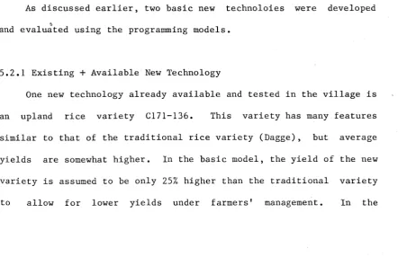
The rainfall pattern is quite similar to most of the upland rice
growing areas of the country. Typically, there are 5 to 7 months of
%
wet season starting in May with at least 200 mm of rain per month
while it is relatively dry during the ret of the year. Figure 2.2
shows the rainfall pattern (26-year average) in Ambulong
(approximately 4 km from Cale), and the 4-year rainfall pattern in
Cale for the period 1974-77.
Crop seasons are defined as early, mid and late wet season. The
weekly mean rainfall fluctuates because of typhoon occurrence in July
to November. The probabilities of obtaining at least as much as the
Rainfall (mm)
1974-75 Cale
J— I_ L
1976-76 Cale
1976-77 Cale
1949-74 Ambulong
Apr May Jun Jul Aug Sep Oct Nov Dec Jan Feb Mar
MONTHS
Fig. 2.2: Rainfall for Ambulong (26-year average) and Cale (1974-77),
Tanauan, Batangas.
[image:22.561.51.518.89.790.2]30% for May, June, November and December and 40% for July-September,
indicating relative variability during different months (Samson et
al. , 1976 , p.3).
2.2 FARM CHARACTERISTICS AND CROPPING PATTERNS
The IRRI’s work in the village started with a baseline survey of
100 randomly selected farms. Data were gathered on crop production
and other aspects of the farming system. Ninety of these farmers had
agreed to participate in the farm record-keeping project, to be
managed by the Economics component of the project. These farmers were
stratified based on the cropping patterns, general standard of living
and other characteristics, and a total of 50 farmers were selected to
participate in the farm record-keeping project. Fifty farmers
participated for two years (1973-75); but only thirty-five farmers
were retained in the project in the last two years (1975-77).
Table 2.2 shows the 1973 baseline information on the 35 farmer
co-operators of the village. The average education level of the
farmers was 3.5 years in school. The average farm size was 1.25
farmers, and many farmers had at least one working animal used in the
farm.
Fourteen per cent of the farmers owned all the land they
cultivated and 51% of the farmers were share tenants, the others
having a mix of fully-owned and tenanted land. The tenancy
arrangement varied between farms. In all arrangements, the farmers
paid the pre-harvest expenses, i.e. fertilizers, chemicals, and
pre-harvest labour. The harvest and post harvest expenses (which also
includes marketing costs) were paid by the farmer from the crop
harvested) which is the common practice for rice or in cash (value of
the crop share) in the case of corn and vegetables.
TABLE 2.2
BASELINE INFORMATION OF 35 CO-OPERATING FARMERS, CALE, TANAUAN, BATANGAS, 1973
Item Mean
Age of Operators (Years) 48
Number of Years in School 3.5
Size of Family 6.4
Farming Experience (Years) 22
Number of Working Animals 0.8
Farm Size (Hectares) 1.25
Tenure Number Per Cent
Owner 5 14
Share 18 51
Owner cum Share 11 32
Owner-Share-Leasee 1 3
Source: Frio and Price (1979).
Table 2.3 shows the percentage of land planted to various
cropping patterns for 1973-77. In all years more than 70% of the
total cropland was planted to a rice-based pattern. The relative
importance of rice in the diet of the villagers may explain their
preference for this pattern. Of these, the rice-corn pattern occupied
TABLE 2.3
PERCENTAGE OF LAND PLANTED TO VARIOUS CROPPING PATTERNS, 35 FARMS, CALE, TANAUAN, BATANGAS, 1973-77
Cropping Pattern 1973-74 1974-75 1975-76 1976-77
Rice-Corn 57 52 53 63
Rice-Vegetables 23 33 21 14
Trellis Crop 5 5 5 4
Corn-Corn 3 1 3 3
Corn-Vegetables 3 1 3 4
Vegetable Intercrop 3 3 3 4
Single Crop 3 3 3 2
Vegetables-Vegetables 2 4 1
Rice/Corn with Relay Crop 1 5 5
Total 100 100 100 100
a) Less than 1%.
b) Vegetables include cowpea, mung, bitter gourd, tomato, sponge
gourd, garlic, bottle gourd, etc.
c) Vine crops are grown simultaneously or in sequence throughout the year.
d) Vegetables intercropped with other vegetables or vines.
e) Crops grown in monoculture and are cultivated the year round, i.e. eggplant, sweet pepper, cassava.
f) Relay crops include sponge gourd, hyacinth bean, bottle gourd
planted shortly before harvesting the first crop.
Source: Frio and Price (1979).
The rice-vegetables pattern ranked second in terms of area
planted. Vegetables were the main source of cash income for the
consumption.
The trellis crop patterns were third in terms of planted area.
Here the crops are grown simultaneously or in sequence throughout the
year. Permanent posts and wiring trellis are constructed to support
the growth of climbing vegetables. However, while this system is
highly profitable, many farmers do not practice this system presumably
because of high initial costs of constructing the trellis.
2.3 LEVEL OF RESOURCES USED
In rainfed agriculture the intensity of land use is entirely
dependent on the amount and timing of rainfall. Table 2.4 shows that
the total cropped area and multiple cropping index varied throughout
the period mainly due to a variation in rainfall.
TABLE 2.4
TOTAL CROPPED AREA, FARM SIZE AND MULTIPLE CROPPING INDEX 35 FARMERS, CALE, TANAUAN, BATANGAS , 1973-77
Year Total Cropped
Area (Has.)
Total Farm Size (Has.)
Multiple Cropping Index
1973-74 71.73 46.73 153
1974-75 64.87 47.79 150
1975-76 56.55 46.14 123
1976-77 58.87 42.68 138
Source: Frio and Price (1979).
The rainfall pattern for 1974-77 (Figure 2.2) shows a high degree
of variability within a month and between months. In 1975-76, after
[image:26.561.58.503.260.768.2]declined very rapidly in late October to early November. The lack of
sufficient soil moisture decreased the area double-cropped in that
year. The same pattern was also observed in 1977.
Changes in the allocation of inputs to different crops and crop
groups are shown in Table 2.5. Fertilizers used for crops increased
over the period. Most fertilizers was applied to high valued
vegetable crops.
Farmers use both family and hired labour. Hired labour
contributed more than 50% of the total labour used in rice in most
years. Most of this labour was spent on hand weeding, harvesting and
threshing. Hired labour for hand weeding came from landless labourers
in the village. Harvesters and threshers came also from nearby
villages. In other crops, hired labour use was very low.
The distribution of farm labour by task for major crop groups is
shown in Figure 2.3. Harvesting required from 34% to 65% of the total
labour used in each crop. Except for corn, where yields increased
over the period, the level of harvesting labour in other crops varied
from year to year, depending on yield levels. Vegetables required
frequent harvesting.
In vegetable cultivation, crop maintenance tasks, such as
weeding, fertilizing and spraying utilized most labour. Generally,
weeding labour varied for all crops from year to year.
2.4 YIELD AND OUTPUT PRICES
Table 2.6 shows the changes in yield of different crop/crop
groups for the period 1973-77. Yields of all crops fluctuated from
year to year. The yield variations are very much related to changes
CN a < H M e a n 5 3 7 5 8 9 9
7 v£> -J- c*1 vO ■<r vo i— <r
CO 00 00 X
o 64
1
2
4 76
1
2
4 2 2
1
0 2 00 00 o oo
ON ON ON ON
ON 1 0 8 1 4 4 1 1 1 1 3
1 On sT
rH co hON CO ON m n co m
oo 44 32
1
2
0
9
5 CN CN o <r
m h CM CN ^ CO CO NCO co o o
a o O 8 1 9 7 [4 3 [3
4 H H CM H 66 66 86 66
ex
o
^
32 7 3 7 6 L 3 3 2 2
3 0 0
9 8 7 7 1 0 0 1 0 0 'ex
o
21
cO <Ub0u m u vO 4 IT) 1— co r-H O CN rH ON O 00 ON 00 ON ON ON
aj
a
P
e
i
CN v£> UO ON
h m cm CL,cu O O ON o
1 0 0 1 0 0 9 1 1 0 0
CO 76 71
1
0
3
1
0
9 s£> rH vO
CN co CN CN 73 64 79 74
CO WO vO CO rH O UO CO
9 9 1 0 0 9 5 9 7
CN rH rH VO VO
S
4 7 4 2 5 3 66 CN NT CN CO
m co m m CO ^ CO fN ^ vO <T
W) CO
X« M 0 3 o o X X C CO
u *H
4-»
<D
•u jH
3
ex J-t
0) 0 N CO *rH u
^ H"3
>h Mvf n 'ü N -o0J s f m vo n rH <r m vo n rH bO
*H o U rH H -H
r^» ! 1 1 1 CO sT IT) vD i—
H H 0 *H
X co <r m o1 1 1 1
1
Xr^- r^. 1 1 1 1 co <r m x r>. O ^
X ON ON ON
on
3
< ON ON ON ON XON ON On ON
W a 2 <0 u c
h o 4-» *J C CO W *H C
OJ H ^ ^
X X 4-J 6
a CO -H O
Ü U J U I a) •u bO C 0»
o a) ^ h
0 > o x w
Ui U CQ -rH 1 iJ \ ^ H X *H a) CJ r-H rH 3 u bO 0 ) 3 l-l -rH O H
Ä ^ a > H
vO oo on O
cn a>
|
a b0 > a-0 o a> •Uo Cß V)
✓—v ^-N CX
a ■u >* O V
<D in H C 3 "O U -H
"a. R ic e C o rn C o rn F ie le L e a
Inter-cultivation
3
HarvestingCROP YEAR
RICE
CORN
VEGETABLES
OTHER CROPS
RICE
CORN (Weeding less than 1%)
VEGETABLES
OTHER CROPS
RICE
CORN (Weeding less than 1%)
VEGETABLES
OTHER CROPS
RICE
CORN (Weeding less
than 1%)
VEGETABLES
OTHER CROPS
10 20 30
— 1--- 1--- 1--- 1_______ I_______ I_______ i
40 50 60 70 80 90 100
Fig. 2.3: Percentage of total labour manhours for various crop
operations spent on each crop, Cale, Tanauan, Batangas, 1973 - 1977.
[image:29.561.26.518.45.741.2]TABLE 2.6
CHANGES IN YIELD OF DIFFERENT CROP/CROP GROUPS, 35 FARMS, GALE, TANAUAN, BATANGAS, 1973-77
Crop/Crop Group
1973-74
Year
1974-75 1975-76 1976-77
1. Rice 1.96
Tons Per
1.05
Hectare
1.80 1.95
2. Corn (wet) 1.08 1.67 1.75 2.20
3. Corn (dry) 1.81 2.46 4.16 3.27
4. Field Crops 0.32 0.76 1.33 0.86
5. Leaf-Vine Stem Vegetables 2.94 7.32 7.49 7.16
6. Bulb-Root-Tuber Vegetables 3.18 5.50 1.59 1.73
7. Fruit Vegetables 8.77 6.95 14.08 7.78
8. Rice/Corn with Intercrops 2.82 2.90 5.77 3.16
9. Vegetable Combinations 9.37 11.62 10.88 6.15
10. Trellis 9.66 10.93 9.38 6.71
Source: Frio
Wet season corn was the only
and Price
crop that
(1979).
showed a steady increase
in yield. Vegetable yields fluctuated widely while rice yields were
relatively stable. Net season corn yields were generally lower than
dry season yields, but were less variable.
The farmers have two markets for their produce, the Tanauan
public market and Divisoria market in Manila. A big truck usually
comes to the village every day to take farm produce to Manila. A
farmer can either sell directly or through a middleman who is paid for
his services. Farmers who sell their produce in Tanauan use jeepneys
received by farmers in Tanauan. However, the price paid by Manila
dealers in the village is lower than Tanauan market prices. Even when
transport costs to Tanauan are taken into account, most farmers feel
it is more profitable to take their produce to Tanauan and sell it
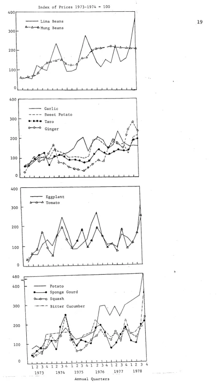
there. Prices of selected crops in Manila are shown in Figure 2.4.
Prices of vegetables in particular showed higher fluctuations
(i.e. eggplant, tomato, sponge gourd, bitter gourd and lima beans),
while prices of non-perishable crops showed least fluctuations
Lima Beans
Hung Beans
Garlic
Sweet Potato
Taro
Ginger
Eggplant
Tomato
--- Potato
•----• Sponge Gourd
o— o— o Squash
--- Bitter Cucumber
JJ
/ ° x1 2 3 4 1 2 3 4 1 2 3 4 1 2 3 4 1 2 3 4 1 2 3 4
1973 1974 1977
Annual Quarters
[image:32.561.68.516.9.803.2]CHAPTER 3
DECISION-MAKING UNDER RISK
In this chapter various aspects of decision-making under risk are
discussed. In Section 3.1, the concept of risk and uncerainty is
given. The main sources of risk in agriculture and the criteria or
rules often used for risky decision-making are considered in Sections
3.2 and 3.3 respectively. Some of the widely used approaches for
accounting for risk in farm decision-making and some of its
applications to agricultural problems are considered in detail in
Section 3.4.
3.1 CONCEPT OF RISK AND UNCERTAINTY
F. Knight (1921) distinguished between 'risk' and 'uncertainty'.
Risk refers to the situations in which alternative outcomes exist with
known probabilities, and uncertainty to situations where probabilities
for the outcomes are unknown.
In modern decision theory, the above distinction is no longer
used. Uncertainty refers to all situations where a single action may
lead to alternate consequences, and risk refers to a characteristic of
the subjective probabilities over the consequences associated with an
action (Roumasset, 1976). Common measures of risk are: (a) variance;
3.2 SOURCES OF RISK IN AGRICULTURAL PRODUCTION
3.2.1 Yield Risk
Yield risk arises from many sources including: (a) variability
in the weather and climatic factors; (b) plant pests and diseases.
The incidence of pests and diseases can be controlled by protective
measures such as spraying pesticide. However, variability in the
weather lies outside the farmers’ control. Among these factors,
rainfall is the most important in our study area, as it has a
completely rainfed agricultural system.
Both the timing and the amount of rain are crucial factors that
contribute to risk associated with rainfall. The Philippines is
frequently visited by tropical cyclones, locally termed typhoons.
Typhoons often result in serious flooding, and also destroy the crops
due to the strong winds associated with them. Floods can cause delays
in the establishment of the crop, and postpone the performance of crop
maintenance operations such as weeding, fertilizing and spraying.
Besides the damaging effects cited above, the amount and timing
of rain can significantly affect the planting calendar of the farmers.
A late onset of rain will delay the planting of the first crop which
in turn 4also delays the second crop. The delayed planting of the
first crop can decrease the yield by increasing the probability of the
crop being exposed to drought stress during the late months of the
season, thus affecting the plants during the reproductive and fruiting
stages of the crop. The yield reducing effect on the second crop
would be through shortening the time in which water can be available
3.2.2 Price Risk
The price risk includes both the input and output price risk.
Roumasset (1976) in his study of risk in decision-making of low rice
farmers in the Philippines excluded the output price as a source of
farm risk. He argued that price risk is generally small in comparison
to yield risk and that in the case of rice and corn, prices were
highly predictable. This is because these crops are government
controlled, and hence will not fluctuate very much. In this study
area, however, output prices is an important source of farm risk.
This is because apart from rice and corn, prices of other crops, such
as vegetables, produced in the farm are subject to considerable
variations other than normal seasonal fluctuations. Despite this,
most of the farmers grow vegetables, due probably to the following
reasons: (a) they are profitable; (b) they can give regular incomes.
Input price risk is generally low in the study area. According
to O ’Brien (1978), (a) prices of inputs such as fertilizers and
chemicals are known with certainty because most farmers buy these
inputs at the start of the planting season; (b) all other factor
payments such as landlord shares and land rents are fixed; and if
altered, are arranged before the planting season; and (c) although
the price of labour (wage rate) is increasing each year, it does not
change within one cropping season.
3.3 CRITERIA FOR RISKY DECISION-MAKING
A decision problem arises when the decision-maker is uncertain
about the consequences of his alternative courses of action. In
decision theory, the decision-maker is usually supposed to act in
of criteria that the decision-maker makes his choice among alternative
decisions. The most common choice criteria considered in theories of
risky decision-making are disussed below.
3.3.1 Expected Profit Maximization
In one criterion, that of expected profit maximization, the
course of action with the greatest expected return (profit) is adopted
irrespective of risk or variability associated with that return. This
criterion is appropriate for decision problems where risk is not a
factor, or when the decision-makers are risk neutral.
3.3.2 Expected Utility Maximization
The criterion of expected utility maximization has been strongly
proposed as an alternative to maximization of expected profit in risky
decision problems (Anderson, Dillon and Hardaker, 1977). The
criterion is based on the expected utility theorem, or Bernoullis'
principle, which states that: given a decision-maker whose
preferences do not violate a set of axioms (discussed below), there
exists a function U, called a utility function which associates a real
number or utility index with any risky prospect faced by the
decision-maker. The theory thus provides a mechanism for ranking
risky prospects in order of preference, the most preferred prospect
being the one with the highest utility. It brings together in an
explicit way the decision-maker's degree of belief and his degree of
preference.
The postulates or axioms (also known as von Neumann and
Morgenstern axioms) for deducing the expected utility theory for the
(a) Ordering and transitivity
A person either prefers one of the two risky prospects a. and a2 ,
or is indifferent between them. The extension of ordering is
transitivity or orderings of more than two prospects, i.e. a , a2 , a 3.
This implies that if a person prefers a 3 to a2 (or is indifferent
between them) and prefers a 2 to a 3 (or is indifferent between them),
he will prefer a i to a 3 (or be indifferent between them).
(b) Continuity
If a person prefers a l to a2 to a 3, a subjective probability
P(a1) exists other than zero, or one such that he is indifferent
between a 2 and a lottery yielding a Y with probability P(ax) and a 3
with probability 1-P(a1).
(c) Independence
If a l is preferred to a 2 , and a 3 is any other risky prospect a
lottery with a 1 and a 3 as its outcomes will be preferred to a lottery
with a 2 and a 3 as outcomes when P(a3) = P(a2). In other words,
preference between a 1 and a 2 is independent of a 3.
The acceptance of the above axioms implies the existence of the
utility function. One important property of this function is that the
scale on which the utility is defined is arbitrary. In particular the
property of this function that is relevant to a choice or decision
analysis is that it is not changed under a linear transformation.
Because of this characteristic, the general shape of the utility
function is not dependent on the origin, and the scale chosen.
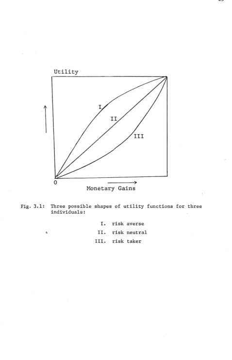
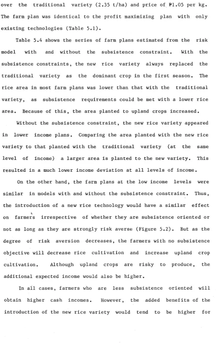
The risk attitudes of the decision-maker determines the shape of
the utility function. Given the utility function U = f(M), where M is
the monetary gains, the function can have any of the three types of
Fig. 3.
Utility
0 --- >
Monetary Gains
: Three possible shapes of utility functions for three
i n d i viduals:
I. risk averse
^ II. risk neutral
[image:38.561.32.511.47.791.2]functions are increasing monotonically throughout, i.e. dU/dM > 0
which means that the marginal utility of income is always positive.
The figure shows that the marginal utility of an additional dollar
varies among the three individuals.
Individual I has a decreasing marginal utility, i.e. d 2U/d2M > 0,
which indicates that as dollar gains increase, they become
subjectively less valuable. This individual falls into the category
of risk averse or risk evader in the sense that in a risky situation
he prefers the action with lower variability for a given level of
expected return.
Individual II, however, has a constant marginal utility of money,
i.e. d 2U/d2M = 0, which indicates that this individual values an
additional dollar just as highly, regardless of whether it is the
first dollar or the 100th dollar. This individual then is considered
to be risk neutral because in the face of a risky situation he ignores
variability.
On the other hand, individual III has an increasing marginal
utility of money d 2U/d2M > 0. This individual will gamble or take a
bet even if the expected value of the outcome is negative. This
individual falls into the category of risk taker or risk preferrer, in
the sense that he will tend to pick an action with greater variability
at the same expected monetary gain.
3.3.3 Security/Safety First Rules of Thumb
These rules of thumb are not derived from Bernoullian utility
functions, although in some cases, it is possible to relate the
optimal allocation decisions to equivalent decisions based on such
Section 3.4.3) that highlight the security desires of decision-makers
by focusing attention at crucial (but generally arbitrary) levels in
the lower tails of probability distributions (Anderson, 1979, p.47).
3.4 THREE WIDELY USED APPROACHES FOR ACCOUNTING FOR RISK IN FARM DECISION-MAKING1
3.4.1 Mean Variance (E-V) Approach
The use of the mean variance (E-V) approach assumes that the
decision-makers maximize expected utility and that either the utility
function is quadratic with respect to expected income and variance of
income or the distributions are normal (Borch, 1969; Feldstein,
1969). Markowitz (1952) introduced the approach in the context of the
choice of the optimal stock market portfolio. He suggested the use of
quadratic programming (QP) to find the most efficient portfolio. He
defined a portfolio as efficient if: (a) no other portfolio with the
same return has a lower variance (or standard deviation); and (b) no
other portfolio with the same variance has a higher rate of return.
Based on this definition, given two portfolios with the same mean
return (E) an investor will prefer the portfolio with the lower
standard deviation, and of the two portfolios with the same standard
deviation, he will prefer the portfolios with the higher E.
Given a set of efficient portfolios, the choice of these
portfolios to any investor will, however, depend on his preference
between various expected returns and associated variance, as described
by the E-V utility function. An investor who is indifferent or
prefers risk will put all his wealth into one security. If he is
1. For detailed reviews of incorporating risk into programming models
see Anderson, Dillon and Handaker (1977), Hubbard (1977), and
indifferent it will be the one with the highest rate of return
regardless of risk.
Since many of the decisions facing the farmers will also involve
a choice of an enterprise mix to a farm, the use of this approach was
extended to agriculture. The first programming model explicitly
incorporating risk in agriculture was done by Freund (1956). He used
the QP to find the optimum combinations of crops for a representative
Eastern North Carolina farm. In this study he found that the expected
net revenue and standard deviation of net revenue from crop
combinations obtained from the QP program were much lower than that
obtained from non-risk programs (ordinary linear programming).
Furthermore, he found that the combination of high risk crops will be
reduced in the QP results. Since their studies of risk in agriculture
has been numerous (for a review see Anderson, Dillon and Rardaker,
1977). A recent study by Rajagoapalan and Varadarajan (1978) in Tamil
Nadu, India, used the QP to measure the impact of technology on farm
risk and evaluated the economic benefits of formal and informal
methods of risk management. One difficulty, however, of using the QP
is the need for a non-linear programming algorithm with desired
features and capacity. Because of this problem a number of linear
approximations to quadratic functions has been proposed.
An alternative approach to QP was proposed by Hazell (1971), the
Minimization of Total Absolute Deviation (MOTAD). In this approach
the mean absolute income deviation was used as a measure of risk.
This approach can be solved on ordinary linear programming (LP)
algorithms with parametric option. A more detailed discussion of this
approach is presented in Chapter 4.
separable programming. In this approach the non-linear variance
constraint is replaced by a piece-wise linear approximation which can
be solved by a linear programming code. As with QP, it selects farm
activities which are efficient in terms of expected income and income
variance.
Chen and Baker (1974) on the other hand have proposed the use of
the marginal risk costraints (MRC) approach which can be fitted into a
linear model with dichotomous MRC, along with the usual resource
constraints. The MRC uses a multistage LP algorithm to approximate
the E-V boundary. In this approach it is assumed that the investor/
decision-maker maximizes the expected return provided that the
marginal contribution of each activity to the total variance of return
does not exceed its expected unit of income, divided by a risk
aversion parameter.
Driver and Stackhouse (1976) also suggested an approach called
linear programming-risk simulation (LP-RS). In their approach the
LP-RS model evaluates the relative riskiness of individual activities
by discounting the expected gross margin in correspondence to its
variation given by the standard deviation. Risk discounting forces
alternate planning solutions with unique resource utilizations,
activity combinations and levels, expected net farm incomes, net cash
position and standard deviation of expected net farm income. The
model derived the E-v^ over the range of expected net farm income (E)
- standard deviation
(/v)
combinations.A rather useful approach is Monte Carlo Programming (MCP) which
was developed by Donaldson and Webster (1968). In the MCP the
portfolio of activity levels are selected at random using a computer.
evaluated in terms of some specific objective function. A large
number of such portfolios can be inspected and the optimal one can be
chosen by the decision-maker. The advantages of this approach are:
(a) that it is very easy to take into account integer constraints on
activities; and (b) that almost any form of objective function can be
applied. In particular, the utility function defined in terms of the
mean and variance of total revenue is readily computable and in
principle higher order moments of the distribution can be accommodated
(Anderson et al., 1977). As in QP, the efficient set of portfolios
can be represented by an E-V utility function. The actual
applications of the approach are still quite limited. Anderson (1975)
has used the MCP to generate many near optimal plans and used the
stochastic dominance rules to select the most risk-efficient plan.
3.4.2 Stochastic Dominance Rule2
Hadar (1971) has defined the general idea of stochastic dominance
(SD) to consist of rules of identifying unamimous preference by a
group of agents or utility maximizers among completely specified risky
prospects (cited in Anderson, 1979, p.51). The application of SD to
portfolio choice was proposed over the E-V approach because the
constraints placed on the utility function by the various dominance
criteria (FSD, SSD, TSD) are more theoretically appealing than the
assumptions of a quadratic utility function, i.e. increasing risk
q
aversion with increasing wealth or normal distribution of returns.
The SD rules are based on the following dominance conditions.
Firstly, define the following variables:
2. Discussion draws heavily on Anderson, Dillon and Hardaker (1977)