Simulation of a beef production system in the moist subtropics

Howard Jeffery

This thesis is submitted in partial fulfilment of the requirements for the degree of Doctor of Philosophy in the Australian National University

Page Acknowledgements

List of Tables List of Figures Summary

Chapter 1 - INTRODUCTION 1

Definitions 2

Complexity 3

The Modelling Team 4

A Final Warning 5

References 7

Chapter 2 - THE CLIMATE GENERATOR 10

Rainfall Generation 13

Temperature 20

Evapotranspiration 21

Soil Moisture Budget 28

References 30

Chapter 3 - THE PASTURE SUB-MODEL 33

Environmental Effects 35

Effect of Temperature 35

Effect of Transpirat ion 39 Effect of Amount of Tissue 40

Effect of Fertility 42

Transfer between the Plant Pools 44

Senescence 46

Decay 47

Competition 47

References 50

Chapter 4 - THE ANIMAL SUB-MODEL 55

Diet Selection 57

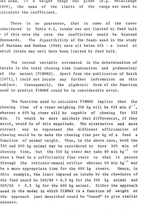
Determining Intake 64

Adjusting Intake for 69

Chapter 5

Chapter 6

Chapter 7

Appendix Appendix Appendix Appendix

Diet M e t a b o l izability and Energy Partitioning

Lactation

Protein Deficiency References

- VALIDATION AND TUNING

Va l i d a t i o n of the Soil Moisture Sub-model Total Model Validation References

- SENSITIVITY TEST

Sensitivity to M a x i m u m Pasture Growth Rate

Sensitivity to Growth Rate/ A v ailability Function Sensitivity to Rainfall Run-off System Testing

Results of the System Test References

- GENERAL D I SCUSSION AND CONCLUSIONS References

A

B

C D

/ 5

76 80 89

96 100

102 124

125 127

130

136 141 14 5 149

This study was supported by a post-graduate study award from the Commonwealth Extension Services Grant (CESG) and by the NSW Department of Agriculture. I am grateful to both CESG and the Department for their assistance and also to the Director-General of the Department for the study leave granted. Much of my time was spent at the Division of Plant Industry, CSIRO, Canberra; I thank the Chief for allowing me to use the Divisions facilities and services.

Many individuals contributed in a number of ways to the completion of this thesis. Thanks are due to Mr. D.A. Gilmour, Queensland Department of Forestry for the provision of soil moisture data; Dr. G.J. Murtagh and Mr. R.J. Martin of the Agricultural Research Centre, Wollongbar for the supply of meteorological records and pasture growth data respectively; Dr. D.W. Turner and Mr. D.O. Huett of the Agricultural Research Station, Alstonville for the provision of meteorological and pan evaporation data. Several colleagues at the Cunningham Laboratory, Brisbane, generously allowed me both their time and data. In particular, Dr. R.J. Jones and Dr. T.H. Stobbs should be mentioned. At Canberra I was provided with an insight into many problems by workers such as Mr. P.M. Fleming, Division of Land Use Research, CSIRO and the following members of the Division of Plant Industry: Mr G.T. McKinney, Mr. C.T. Gates, Dr. M. Freer and Mr. F.X. Dunin. I am grateful to my fellow student, Mr. D.H. White of the Victorian Department of Agriculture, for the many valuable hours spent discussing numerous aspects of modelling. A number of members of the Department of Environmental Biology, ANU, made useful suggestions and provided helpful advice.

The Fortran that I know is largely a product of the patience and knowledge of Mr. J.S. Armstrong, CSIRO, Division of Plant Industry.

The graphs reproduced in the thesis were produced by a program written by Mr, G. Knowles, Research School of Biological Sciences, ANU. I am thankful for the help he gave me in implementing and, when necessary, altering the program.

It is with deep gratitude that I acknowledge the generosity of Dr. P.T. Hears of the Agricultural Research Station, Grafton in the unsparing provision of his data. My requests for greater details of the data were always promptly granted. This data was essential for the validation of the model.

I am acutely aware that but for the contribution of my supervisors this thesis would have taken longer to complete and would have made an even smaller contribution. My most sincere thanks are given to Dr. F.H.W. Morley, Division of Plant Industry, CSIRO and Professor R.O. Slatyer, Department of Environmental Biology, ANU. Their guidance was always offered in a true spirit of scholarship and its impact often extended beyond the bounds of biology. During periods of absence of Professor Slatyer, Dr. B.R. Trenbath, Department of Environmental Biology was an acting supervisor, although Dr. Trenbath actively assisted and encouraged me over the total period of study.

2.1 Constants used to define the moisture 29 characteristics of the soil.

3.1 Temperatures used to define the 38 growth/temperature relationships.

4.1 Botanical composition (in kg ha- 1 ) 58 of a hypothetical sward.

4.2 Values of FRCINT calculated from the 61 hypothetical sward.

4.3 Botanical composition (in fractions) 61 of the hypothetical sward.

4.4 Mean nitrogen content of the pasture 63 species at two levels of soil nitrogen.

4.5 Estimates of the coefficient, relating 67 metabolizable energy intake to weight

raised to the .75 power.

4.6 Reported and derived estimates of 72 the effects of lactation and

pregnancy on dry matter intake.

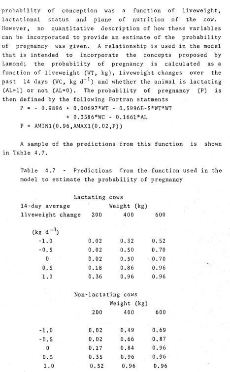
4.7 Predictions from the functions used 83 in the model to estimate the

probability of pregnancy.

5.1 Treatment combinations used in the 102 experiment of Mears (1973) .

5.2 An example of the calculation of the 105 objective function used in the model

validation.

5.3 An examination of the between-plot 116 variation in liveweight gain.

5.4 The mean differences between the 121 experimental data and the model.

6.1 The three years simulated rainfall 127 used in all sensitivity tests.

6.2 The sensitivity of the model to 128 decreasing and increasing maximum

pasture growth rates by 20%.

6.5 T h e e f f e c t o f i n c l u d i n g a r u n - o f f f u n c t i o n in t he m o d e l .

138

6.6 T r e a t m e n t s c o m p a r e d in the s y s t e m

t e s t of the m o d e l .

142

6.7 E c o n o m i c a n d e n e r g y c o s t s u s e d in

the a n a l y s e s .

144

6.8 S u m m a r y of t h e t r e a t m e n t m e a n s f or

s e v e r a l of t he b i o l o g i c a l v a r i a b l e s .

146

6.9 S u m m a r y o f t he t r e a t m e n t m e a n s f o r

2.1 Flow-chart of the climate generator. 14 2.2 Probability of rain on a given day. 16 2.3 Histogram of the frequency with which 18

different daily falls of rain were recorded in January.

2.4 Mean rainfall on days when rain 19 was recorded

2.5 Mean temperature and standard 22

deviation of mean daily temperature.

2.6 The relationship between actual 26 evapotranspiration from a 12hr-daylength day and maximum transpiration rates.

2.7 The relationship between the ratio of 27 actual/potential evapotranspiration

from a 12hr-daylength day and maximum transpiration rates.

3.1 Flow-chart of the pasture sub-model. 34

3.2 The temperature/plant growth 36

relationship

3.3 The components of a very simple 45 plant growth model.

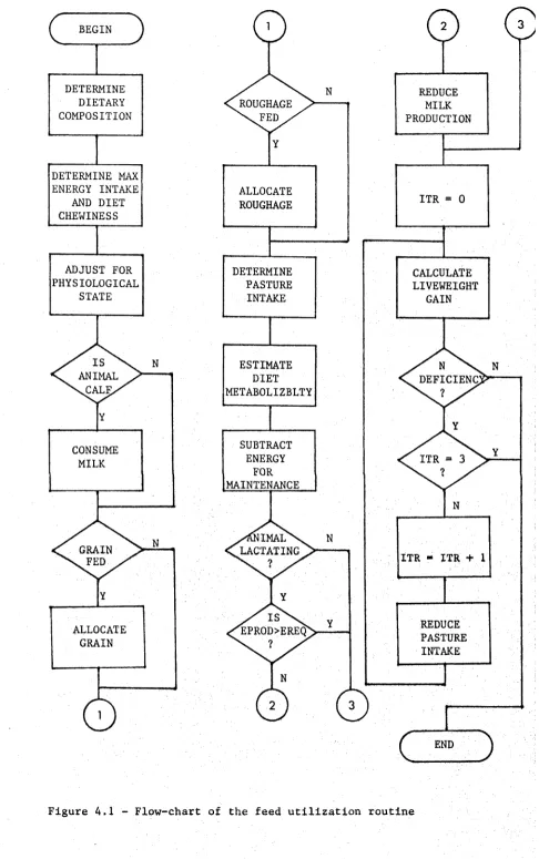
4.1 Flow-chart of the feed utilization 56 routine.

4.2 The statement function CELECT which 60 is used in the determination of the

botanical composition of the diet.

4.3 Proposed relationships in the 65 regulation of food intake in cattle.

4.4 Feed intake of all-roughage diet 70 observed by McCullough (1969).

4.5 The potential milk production of 78 a cow giving a maximum yield of 10kg.

4.6 The relationship between liveweight 85 of a cow and calf birthweight.

5.2 A comparison of the model output 107 and observed values of four treatments

from the low fertility replicate.

5.3 A comparison of the model output 113 and observed values of four treatments

from the high fertility replicate.

6.1 The relationship between growth rate 129 and pasture availability; maximum

growth rate from the lower curve is 80% of that for the upper curve.

6.2 Growth rate/availability responses for 132 different settings of the parameter m

of Richards (1959) .

6.3 Increase in availability from a low 133 availability for different values of

the parameter m of Richards (1959) .

6.4 The relationship between run-off 137 and rainfall.

6.5 The soil moisture profiles in years 139 1 and 3 when the run-off routine was

A simulation model of a beef farm on the far north coast of NSW was constructed and validated. The final version was used to examine the consequences of altering time of calving, stocking rate and rate of nitrogen fertilization over a three-year period.

The model was composed of three major sections: a climate generator, a pasture generator and an animal sub-model. The climate generator reproduced what appeared to be realistic rainfall patterns using a first-order Markov process to generate rainfall conditional on whether rain fell on the previous day or not. The probabilities of rain falling were derived from historical data. The mean daily temperature was also generated and the combination of mean temperature, day of the year and whether rain fell or not was used to predict pan evaporation - this equation was developed from data obtained in the region under study. Actual evapotranspiration was calculated on a daily basis, but used a method which considered the evaporative demand pattern within a day. When this method was incorporated with the soil moisture routine good agreement was obtained between the model and some Canberra data.

The pasture was taken to be composed of four competing pasture species : Axonopus affinis, Paspalum dilatatum, Pennisetum clandestinum and Trifolium repens. Competition between these species depended on the growth rate of each species, the fraction of ground cover it occupied and the nitrogen content of the soil. Growth rate was defined to be a function of available pasture, evaporation ratio (actual/potential evapotranspiration), temperature, and the phosphorus and nitrogen contents of the soil. Provision was incorporated in the model for the application of either phosphorus or nitrogen fertilizers.

daily basis and new material added to pool 1. Each day a transfer of material from pool 1 to 2, 2 to 3 ... 4 to 5 occurred depending on the pasture senescence rate. The rate of transfer out of pool 5 depended on the pasture decay rate.

Animals "grazing” the pasture selected a diet which depended on the amount of material in the various pasture pools. There was a positive selection for material in pool 1 over pool 2, pool 2 over pool 3, ... and a minor preference for clover over grasses. Each pool-species combination had a defined digestibility and fibre content. Feed intake was limited by either the energy demands of the animal being satisfied or the maximum amount of "bulk" being consumed. Provision was made for the consumption of either grain or hay.

Where possible, utilization of feed followed the method defined by the Agricultural Research Council of the UK. An exception to this was in the allocation of nutrients within the animal for liveweight gain (positive or negative) in the lactating cow. A method was developed which allowed a drop in milk production when a poor feed was fed, a permanent drop in the ability to produce milk if a poor feed was fed for long periods, an increase in milk production if a cow's diet changed from poor to good feed and either a positive or negative liveweight change at any stage of lactation. This routine is regarded as being a good prototype for more refined milk production models.

o

treatments arranged in a 3 factorial design (time of calving x level of nitrogen fertilizer x stocking rate). The scale of this simulated experiment was such that it could never be conducted physically as 150 breeding cows were assigned to each treatment. It was concluded from this system test that on both economic and energy cost bases, nitrogen fertilizer had no place in a breeding system on the far north coast of NSW. Time of calving had little influence, though an advantage from late calving may occur. Predictably, stocking rate had a large influence on the economic and the energy cost per hectare.

Chapter 1

INTRODUCTION

Simulation modelling is a relatively new technique to be applied to agricultural management problems. It is seen as having great potential in management studies (Arcus 1963; Morley 1968) and sometimes may be the only feasible approach. This thesis describes the construction and validation of and, finally, experimentation with a model of a beef farm on the far north coast of NSW.

The subject was chosen for two reasons. First, I had just spent a little over four years on the north coast at the Wollongbar Agricultural Research Station and thus had some appreciation of the behaviour of a grazing system in that environment. It was hoped that this knowledge would reduce the number of frangible assumptions incorporated in the model. The second reason was that many advocates of systems analysis (Spedding 1970; Van Dyne 1970, amongst numerous others) have seen one of the applications of simulation being the exploration of potentially important fields in which few data have been collected. Beef systems on the north coast fell into such a category.

Definitions

The term "system" has a connotation to most people, yet, it is doubtful whether the sense in which it is used in the phrase "systems analysis" can be concisely defined. I know of no succinct definition of this term which captures the philosophy of approach the phrase implies to me, nor can I derive one. Dale (1970) observed that systems analysis has rarely been defined when introduced into ecological studies.

Anderson (1974) distinguished between systems analysis and simulation modelling, arguing that the former involves a broader and more philosophical approach. The same distinction will be made in this thesis and the phrases systems analysis, systems approach and holistic view will be used interchangeably. The term "simulation modelling" will be used in connection with the techniques of building a computer model of a system.

No formal literature review has been attempted in this thesis. This decision was made as several recent and comprehensive reviews on the application of systems analysis and simulation modelling to biological fields have been published (Dale 1970; Dent and Anderson 1971; Benyon 1972; Anderson 1974). Three recent publications also provide examples of a variety of applications of simulation modelling to agricultural systems. These publications are the proceedings of a symposium on the use of models in agricultural and biological research held at Hurley in the UK in 1969 and published in 1970, an almost 400 page book edited by Dent and Anderson and published in 1971 and the symposium on systems analysis held in Canberra and published in the Proceedings of the Australian Society of Animal Production

(1972).

of the important ones in the particular fields, but the list is by no means exhaustive.

Complexity

The most consistent feature of expository articles on simulation modelling is the stern warning that undue complexity should not be included in the model (Dent and Anderson 1971; Armstrong 1972; Garfinkel et al. 1972). The next most consistent feature has been the failure to describe how "undue” complexity can be recognised. Extreme examples of degrees of complexity that may be inappropriate are easy to generate and denigrate. In practice the problems are not as clear-cut and the decision will be very much a subjective one. In this context it is probably wise at the outset to accept, as have many others (Garfinkel et al. 1972; Anderson 1974), that simulation modelling is better regarded as an art than as a science. Ironically, simulation modelling usually involves what would be often regarded as the epitome of technology - the electronic computer.

De Wit (1970) saw the problem of complexity in terms of "levels of knowledge" each with its associated "relaxation time". Although no rigorous definition of relaxation time was offered by de Wit, the point of view he was advancing was fairly clear. An example was given of a stomate having a relaxation time of seconds whereas it would take years for a damaged forest to recover. It was thus implied by de Wit that a model of forest regeneration would be unduly complex if it was also concerned with stomate movement. The concept of relaxation times is useful in that it provides a qualitative basis for the estimation of complexity. However, even if relaxation times can be agreed upon the decision as to whether the relaxation times are too far apart will still be subjective.

that of the above models and the IBP model ELM, parts of which were described by Anway (1973) and Sauer (1973).

Several of the variables in the model are stochastic. It was thought that to ignore between-year variability in rainfall and temperature would result in the conclusions being based on unacceptably unreal conditions; rainfall and temperature have thus been included as stochastic variables. Other variables treated as stochastic are the number of cows becoming pregnant during mating and the number of male and female calves born. The major reason for adding a stochastic element to these variables was to allow an examination of some of the consequences of chance variation in a whole-farm context, particularly when herd numbers are small. Although the long-term economic effects of chance variation would be small, it is conceivable that chance variation could have considerable impact over a short period.

The model was written as a series of difference equations and used a one-day time step. One reason for preferring this value to a longer one (which would have used

less computer time) was that the estimation of actual evapotranspiration involves a consideration of the daily pattern of evaporative demand. A one-day time step was also the shortest that could be reasonably considered as the rainfall and temperature records available to me were recorded daily.

The Modelling Team

building and stated that the biologist, who is to be the modeller, can not "expect much help from the mathematician because there are in fact no mathematical problems involved". Morley (1972) presented a similar attitude, whereas economists (Dent and Anderson 1971) appear to adopt an intermediate position.

General agreement on the desirable composition of a modelling team will probably never be reached. However, almost invariably the modeller will need help and guidance from workers in other disciplines (Morley 1972).

A Final Warning

Before commencing the detailed description of the model several preliminaries remain. It is traditional for models to receive a name that is in some way descriptive or is formed from an acrostic. An example of the former is the model of Freer and Armstrong, termed HAGGIS, which simulates ruminal activity. An example of the latter is this model which derives its name, SCREW, from the following:

Simulation of a Cattle

Raising Enterprise

With a digital computer.

The less charitable may also regard this term as being descriptive.

The model is composed of three major sub-models; the climate generator, the pasture sub-model and the animal sub-model. Several trends are evident in this sequence. The data available for analysis and synthesis and the precision with which they have been obtained decrease from climate to plant to animal. Consequently, the representation of the climate obtained from the climate generator is more likely to be a faithful reproduction than is the portrayal of feed utilization contained in the animal sub-model. A further consequence is that the assumptions within these sub-models become more tenuous as the above progression is followed.

Dillon (1971) promulgated three Laws of Simulation. They bear repeating.

(i) Simulation, like statistics, cannot prove anything, (ii) Simulation, like statistics, can nearly prove

anything,

(iii) Once started, simulation will continue until available funds are exhausted.

Anderson (1974) complemented these laws with three hypotheses

(i) Every simulation study has its trenchant critics, (ii) The more aggregative the simulation, the more liable

it is to criticism,

(iii) Study through simulation always absorbs more resources than anticipated a priori.

REFERENCES

Anderson, J.R. (1974) - Simulation : methodology and application in agricultural economics. Rev. Mktg agric. Econ. 42: 3-55.

Anway, J.C., (1973) - Consumer simulation model. A canonical mammal. Proc. Summer Comp. Conf. Vol 2, pp 835-840.

Arcus, P.L. (1963) - An introduction to the use of simulation in the study of grazing management problems. Proc. N.Z. Soc. Anim. Prod. 23: 159-168.

Armstrong, J.S. (1972) - Getting models off the ground, Proc. Aust. Soc. Anim. Prod. 9: 104-111.

Benyon, P.R. (1972) - Computer modelling and interdisciplinary teams. Search 3: 250-256.

Dale, M.B, (1970) - Systems analysis and ecology. Ecology 51: 1-15.

Dent, J.B. and Anderson, J.R. (1971) - Systems, management and agriculture. In, "Systems Analysis in Agricultural Management", Ed. J.B. Dent and J.R. Anderson (Wiley :

Sydney).

Dillon, J.L. (1971) - Interpreting system simulation output for managerial decision - making. In, "Systems Analysis in Agricultural Management", Ed. J.B. Dent and J.R. Anderson (Wiley : Sydney).

Freer, M. , Davidson, J.L., Armstrong, J.S. and Donnelly, J.R. (1970) - Simulation of grazing systems. Proc. XI int. Grassld Congr. pp 913-917.

Garfinkel, D. , McLeod, J . , Pring, M. and DiToro, D. (1972) - Application of computer simulation to research in the

Mears, P.T. (1973) - Effect of stocking rate on the nitrogen

response characteristics of kikuyu fPennisetum

clandestinum) pasture. Ph. D. Thesis, Univ, Qld.

Morley, F.H.W. (1968) - Computers and designs, calories and

decisions. Aust. J. Sei. 30: 405-409.

Morley, F.H.W. (1972) - A systems approach to animal

production. What is it about? Proc, Aust. Soc. Anim,

Prod. 9: 1-9.

McKinney, G.T. (1972) Simulation of winter grazing on

temperate pasture. Proc. Aust. Soc. Anim. Prod. 9:

31-37.

Radford, P.J. (1967) - Systems, models and simulation. Essay

in 1967 A. Rep. Grassld Res. Inst., Hurley.

Radford, P.J. (1970) - Some considerations governing the

choice of a suitable simulation language. In, "The Use

of Models in Agricultural and Biological Research", Ed.

J.G.W. Jones (The Grassland Research Institute : Hurley,

UK) .

Sauer, R.H. (1973)- PHEN : A phenological simulation model.

Proc. Summer Comp. Simulation Conf. Vol 2, pp 830-834.

Spedding, C.R.W. (1970) - The relative complexity of

grassland systems. Proc. XI int. Grassld Congr. pp

A126-A131.

Standen, B.J. (1969) - Changes in land use in the Richmond

Tweed region of New South Wales 1958 to 1967. NSW Dept.

Agric., Div. Mktg Econ., Misc. Bull. 7.

Van Dyne, G.M, (1970) - A systems approach to grasslands.

Proc. XI int. Grassld Congr. pp A131 - A143.

Vickery, P.J. and Hedges, D.A. (1972) - Mathematical

model of improved pasture grazed by Merino sheep. CSIRO, Anim. Res. Lab., Tech. Paper No. 4.

Watt, K.E.F, (1968) - ’’Ecology and Resource Management” (McGraw - Hill : New York).

Wit, C.T. de (1970) - Dynamics concepts in biology. In, "The Use of Models in Agricultural and Biological Research” , Ed, J.G.W, Jones (The Grassland Research Institute : Hurley, UK).

Chapter 2

THE CLIMATE GENERATOR

Two difficult decisions have to be made by the builder of a simulation model which includes climatic input. The first concerns the choice of variables to be included in the model; the second decision is whether the values used will be

a sample of real data or generated data.

Because many climatic variables are highly correlated, e.g. temperature and solar radiation, the exclusion of one variable from the model may have little effect on the output. The exclusion of variables simplifies the model but will reduce the size of the parameter space to which the model can be applied, e.g. a model of plant growth based on soil moisture may give good predictions in say, an arid environment, but it could not be expected to yield good predictions in a cool temperate environment where temperature and solar radiation are more likely to limit plant growth. The final decision about which variables are to remain in the model is a compromise. In the absence of any developed theory on the subject,the decision is a subjective one though factors such as the time step (integration interval) being used, the theoretical significance of the variables and the degree of correlation between variables should be borne in mind when making the decision.

The majority of agricultural models have used historical

data to provide the rainfall input (Freer et al. 1970; Wright

1970; McKinney 1972; Vickery and Hedges 1972; Smith and

Williams 1973). Only rarely have models (Trebeck 1972;

F.H.W. Morley pers. comm.) generated the rainfall data,

although Phillips (1971) argued strongly that this approach

was better.

Phillips’ advanced two arguments. First, an historical

sample of real data cannot give a complete coverage of all

possible values, hence, not all theoretically possible values

have a finite chance of occurring in the model. This, he

argues, makes the variable, which is theoretically

continuous, decrete in practice. The second argument

advanced was that a certain lack of smoothness will almost

certainly occur in the historical data, e.g. there maybe a

greater probability of receiving rain in say, the 30-35mm

range than the 25-30mm range although modal rainfall may be

10mm. Phillips regards this as being due to a fluctuation in

the sampling rather than a lack of smoothness in the

underlying process.

The arguments of Phillips are technically correct but

their relevance may be questioned. Both arguments are

concerned with the extreme values of distributions. At thes#

high levels of rainfall, field capacity is likely whether the

correct or a somewhat biassed estimate of rainfall is used.

As the fate of run-off rainfall is. generally outside the

scope of agricultural management models it is therefore

irrelevant whether run-off is 20 or 25mm.

An advantage of using data obtained from a rainfall

generator is that the sequence of data is controlled by the

random number initiator (seed) of the computer’s random

number generator. Consequently, at relatively low cost a

large number of different yearly sequences of rainfall can be

generated, each sequence being tied to a particular

initiating seed. Thus, the model can be run over say, four

use of a few simple Fortran statements such as DO 100 NYEAR = 1,4

NSEED = NSTORE(NYEAR) CALL RANSET(NSEED)

where NSTORE holds the already determined appropriate seed values of the random number generator. In theory, the same approach could be used with sets of historical data, although storing and manipulating tens of years climatic data would probably introduce some practical data retrieval problems.

If an agricultural management simulation model is to be used in decision-making and has stochastic rainfall input, then the decision must be based on an adequate sampling of years which include variations in the totals and distributions of rainfall. One way of meeting these objectives is for the input data to be a large random sample, e.g. 25 years. Such a sample must be long enough to avoid any undue influence from wet or dry "cycles” within it. Alternatively, the modeller may select years of good, average and poor rainfall and weight the model outputs according to the probability of occurence of good, average and poor years. Rather than ranking years as good, average or poor, the years may be ranked according to the pattern of rainfall within them. For example, the years may be rated as "wet spring" or "dry summer" years and, as in the previous case, the outputs weighted according to the probability of occurence of the so-defined years. Although the last method is similar in principle to the definition of the years as good, average or poor, it has the advantage that the type of year chosen can be of direct relevance to the agricultural system being tested, e.g. years defined as "dry spring" may well be chosen if the associated model is concerned with cereal cropping. The latter two methods, which do not involve random sampling, and may only involve a two or three year run, will use considerably less computer time than the first method which may involve a run of more than 25 years.

and no assumptions need be made about the rainfall probability distribution. On the other hand, it may, but need not, use large amounts of computer storage, and it will probably introduce some practical data retrieval difficulties. If rainfall input is obtained from a rainfall generator, then little computer storage is needed and, as demonstrated above, the rainfall pattern can be easily manipulated. Although not compelling, Phillips’ arguments also provide reasons why a rainfall generator may be preferred. It would be fairly simple to apply a rainfall generator to a neighbouring region which experiences a similar climatic pattern. If few rainfall records exist for this neighbouring region, then the development and ’’extrapolation” of the generator may be preferable to the use of the relatively few, perhaps atypical, records. I can see no simple solution to the question of whether one should or should not use historical rainfall data. In fact, two of the dominant reasons for building a climate generator in this model were strongly personal ones : (i) the building of the generator represented a challenge, and (ii) it appeared to me to be a more elegant approach.

Mean daily temperature, daily rainfall and daylength are the environmental variables generated in the model. Temperature and rainfall estimates are stochastic. The three generated variables, together with the date, allow calculation of potential and actual evapotranspiration and the soil moisture budget. The majority of these calculations are performed in subroutine CLISIM, although it needs the associated function subprograms ANORM and RAINRV, A flowchart of this process is presented in Figure 2.1.

Rainfall Generation

FUNCTION RAINRV

FUNCTION ANORM

SOIL MOISTURE

TRANSFERS CALCULATE

RAINFALL

CALCULATE POTENTIAL AND

ACTUAL £VAPOTRANSPRTN

CALCULATE MEAN TEMPERATURE

Phillips (1971) discussed several methods of sampling

that produce realistic results» These methods included

recursive regression and conditional probability models.

Alternatively, if large enough sampling periods (n days) are

selected, independence of successive sampling periods can be

assumed. Hence, the total rainfall for each n-day period can

be obtained by random sampling. Sampling within each n-day

period can be based on an analysis of historical data to

define the conditional probabilities of m wet days given the

rainfall for an n-day period. Phillips considered that for a

sample of data he dealt with, successive seven day totals of

rainfall could be considered as independent.

A further approach has been used by F.H.W. Morley (pers.

comm.). Whether rain fell or not is first determined and if

it did,then the amount that fell is calculated. This is thus

a two-stage approach as opposed to the more direct methods

discussed by Phillips. The method used in CLISIM is a

two-stage approach; the probability of rain depends on

whether or not rain occurred on the previous day.

Twenty-five years' daily rainfall data were obtained

from the Agricultural Research Station Wollongbar, NSW. The

data were divided into monthly groupings and analyses

performed on data for each month. The procedure followed was

outlined by Gabriel and Neumann (1962) and involved

determining the probabilities of rain conditional on whether

rain fell or did not fall on the previous day, i.e.

p = Pr(wet day | previous wet day)

p = Pr(wet day | previous dry day)

The twelve monthly values of p Q and p were now fitted by the

least squares method to provide the following equations;

Po = .570 + .096*SIN(Z-.133) + .019*SIN(2*Z-1.135)

(R2 = .927)

p = . 216 + . 068 *SIN(Z+.923) + . 009*SIN(2*Z-.495)

(R2 » .971)

where Z = 2n/365*LDAY

LDAY takes the value 1 on Jan 1, 2 on Jan 2 .... 365

These functions are presented in Figure 2.2. Using these equations and the random number generator, sequences of wet and dry days can be calculated. If it is determined that rain fell on a particular day, the next step is to estimate how much fell. This requires knowledge of the rainfall probability distribution.

The probability distribution of rainfall has a positive skew and consequently a number of asymmetric distributions have been used to describe it. F.H.W. Morley (pers. comm,), Walker and Rijks (1967) and the Bureau of Meteorology have used the log-normal distribution although Das (1956) demonstrated that his (Das 1955) use of a truncated Pearsonian type III distribution was more appropriate for the rainfall data of Sydney. Phillips (1971) advocated several other Pearsonian distributions (Types I, IV and VI).

An examination of the distribution of the daily rainfall recorded in each of the twelve months was obtained. These data were plotted as histograms using class intervals of 2.5mm. All plots had a similar distribution in which the ratio of the standard deviation to the mean averaged 1.6 and showed no evidence of seasonal variation. The histogram of the January distribution is shown in Figure 2.3. There was a seasonal variation in the mean rainfall recorded on rainy days. This seasonal variation is described by the variable FXRAIN (Figure 2.4) :

EXRAIN = 12.02 + 2.5*SIN(Z-.02) - 0.98*SIN(2*Z-1.24) (R2 = .818)

where Z = 2n/365*LDAY

F R E Q U E N C Y u i n < ü

-□ h O

S

• T3 O) M 4-1 co 4-i

P *H

c CO l_) c •H TO 01 M3 G O U CU Vh

0) 00

1-1 c

O) -H 3 XJ

1-1 m 01 o c o to r—1 4-1 r—t cO cO ,C cm 4-1 >> 4-1

r-H a ,

•H CU CO u X> X 01 r C u — •H X>

r C 0)

2 4-1

4-1

r C o

4-1 T-4 *H a G <u U 01 C x 0) p CO

c r CO

01 ,G

g

CM CO

1-1

01 CO

r C CU

4-1 Po CM m o CM E E cd O V4 M

RA IN FA LL ON RAI NY D A YS

£1 B ti

Q

O

0)

GO 03

CO U

trial values were evaluated and 2.3 was found to be a suitable power. The random variable generated this way had an expected value of about 1.12. Hence, rainfall is calculated by raising the absolute value of a standard normal variable to the power of 2.3, dividing by 1.12 and multiplying by EXRAIN. This random variable is generated in

the function sub-program RAINRV.

A comparison of the mean monthly rainfall records generated by this method over a period of 200 years showed no significant departure from the twenty-five years’ data on which it was based. The distribution of monthly and yearly totals also appeared realistic. Thus, this method of rain generation was employed in the model. The method of generation is not completely realistic when heavy falls of rain occur. When the region is influenced by a cyclonic depression the chance of heavy falls on successive days is high but this tendency for successive days of high rainfall has not been incorporated into the rainfall generator,This failure to faithfully reproduce rainfall patterns will probably not be important because whether one, or a series of days of heavy rainfall occurs, the soil will reach field capacity. Little reliance can be laid on the fact that the generated data were not significantly different from the observed; the between year variation is such that the 25

2

years’ data from 1911-1935 was found by the X test to come from a different population than the 1936-1960 sequence with a probability of greater than 95%.

Temperature

Between-year variation in mean temperature is relatively smaller than the between-year variation in rainfall. The probability distribution of daily temperature is also more convenient. Thus, generation of realistic seasonal patterns is much simpler for mean daily temperature than for rainfall.

occurred in mid-summer and mid-winter and was about 1 deg. Because differences of this order were not considered likely to have a great affect on the model's behaviour, the assumption was made that no differences existed between the expected temperature on wet and dry days.

The expected temperature (EXTEMP) for any day is predicted from the following periodic equation

EXTEMP = 18.72 + 4.61*SIN(Z+1.287) + 0.59*SIN(2*Z-1.512) (R2 = .998)

whilst the standard deviation of the temperature (SDTEMP) was given by the following equation (Figure 2.5)

SDTEMP = 5.32 - 0.629*SIN(Z-.927) + 0.747*SIN(2*Z-1.396) + 0.496*SIN(3*Z-.380)

(R2 = .693) where Z = 2tt/365*LDAY

The results of Thom (1973) and the plot of the daily temperature data for each of the twelve months, suggested that the temperatures were normally distributed. In the model, the actual deviation from the expected value is calculated by sampling from a normal distribution with standard deviation defined by the above equation. In order to produce a correlation with the previous days' temperature this value is added to the previous days' temperature and the average taken. This procedure lowers the variance of the estimated temperature; however, it was found by simulating this process that multiplying the predicted standard deviation by 1.732 produced data of the correct variability.

Evapotranspiration

T E M P ER AT UR E ( d e g C ) « a o < PE H a o s s < X Pm

UZ

51

DT

0

The first step in such an approach is to predict daily potential evapotranspiration (Et) from daily pan evaporation (E0). The relationship between pan evaporation and potential evapotranspiration is generally assumed to be linear (Slatyer 1967) :

E t = k

,

2

o

where k, is the "pan factor" and k2 the "crop factor". The pan factor is associated with different evaporation pans and depends on the type of pan and its placement (above, at or below the ground surface). The crop factor depends on the plants or sward being considered and their coverage of the ground. Generally, no attempt is made to separate the values of k, or k 2 for simulation studies, as it is their product which is required. Estimates of this product for a sward have varied, with the majority being in the interval (.6,.9). Penman (1948) noted that the coefficient was lower in winter than summer. His results were variable but a difference of about .2 appeared to exist between the seasons. Consequently, the following function is used to define the parameter PENMAN, which is the product of k, and k 2

PENMAN = 0.6 + 0.1*SIN(Z+1.5708)

where Z is as defined above. Hence the summer value for PENMAN is .7; the derivation of this value is described in Chapter 5.

It is worthwhile noting that had a larger value of PENMAN been chosen it could be made to have no effect on the model merely by increasing the size of the soil moisture pool. This is an example, not rare in simulation modelling, where no real gain is obtained from an accurate determination of a single parameter. In this case, if extra accuracy is to be of benefit it must be achieved concurrently in a set of paramters.

POTEVP = 3.28 + 0.Ill*TEMP + 0.00101*TEMP**2 - 1.12*KPREV - 1.13*SIN(Z-1.29)

(R2 = .283) where Z = 2tt/36 5*LDAY

The coefficient of determination of this regression was

3

not substantially improved by either the inclusion of TEMP as a variable or estimation of the second harmonic. Although the coefficient of determination was low, it was not as low as some of the values reported by Fitzpatrick (1963) in which temperature was the only independent variable. The lower values reported by Fitzpatrick also came from a coastal environment whereas inland values were uniformly high (r>.9).

Actual daily evapotranspiration (Ea) is calculated from a consideration of the evaporative demand of the environment and the estimated ability of the plant to meet that demand. Details of the method are outlined in Appendix A and only a summary follows.

If the potential evapotranspiration, daylength and pattern of evaporative demand within a day are known, it is a straightforward matter to calculate the instantaneous rate at which water must be supplied to meet that demand. In particular, if the maximum rate at which a plant can

transpire (dEm/dt) exceeds the rate at which the environment can extract moisture (dEt/dt), then the plant’s actual rate of transpiration (dEa/dt) is assumed to be equal to the environmental demand rate. On the other hand, if dEt/dt exceeds dEm/dt, then the actual rate of moisture loss is assumed to be equal to the maximum rate the plant can sustain

(dEm/dt). This model of transpiration wa^ proposed by Fleming (1964) and can be summarised a>,

dEa/dt = d E t/dt if dEm/dt > dEj/dt dEa/dt = dEm/dt if dEm/dt < dEt/dt

demand made virtually no difference to the estimates of E a, so the computationally simpler method (assuming a cloudy day) has been used in the model. This function is presented in Figures 2.6 and 2.7.

Soil moisture is considered to be held in two layers. Because the density of plant roots is greatest in the top layer, it can provide moisture at the greater rate. The ability to supply moisture declines linearly as soil moisture declines from field capacity to wilting point, as has been proposed by Fleming (1964) and Baier and Robertson (1966). The rates of evapotranspiration at field capacity for the two layers are 1.5 and 0.6 mm hr-1. The ratio between these two values (2,5) is similar to that which gave the best fit to the data of Baier and Robertson (1966) for soil profiles of similar depths. The esimate of 1.5 mm hr-1 as the maximum rate of evapotranspiration is based on rates of this order estimated by van Bavel (1966) using alfalfa. The species and the environment were different from those being considered in the model, nonetheless the estimates of van Bavel provide an indication of the sort of evapotranspiration rates that plants in the field can maintain.

A C T U A L E V A P O T R A N S -P IR A T IO N i n

- T --- 1... ...— ---1--- —

T-C I B t i □

I u r£ E 3 e

•H E X E 03

E c 'V c

C *r

03 4-

Ct >> P

03 •(-

T3 c cr

X p

4-j o:

00 P

C 4-

<U C rH c > > o: cd >

'V a 1

U r

-Oi -r-r—) 4-

p cd a,

4J

c c O P

C <U

U3

C

O *H

■H 4 J

pH *H

cu a H cn

C a) cd H

H 4 J

E V AP O RA TI O N R A T I O in d E o

d -H

E

•H

X

03 -H

E p

w d 03 P XJ d 03

^ C

0) C

X)

>

X a p

Ö O

r-d o

0) *r <—I P

c o3 a

X5 P

I C

p c X

X

C/3 |

d 1

o -i

*H J

P

0} r H •

Soil Moisture Budget

After rainfall, actual evapotranspiration and rainfall run-off have been determined, the estimation of the amount of moisture in the soil becomes a straightforward budgetary exercise (Flinn 1971). The rules for the budget vary between models depending largely on the number of soil compartments considered and the transfers between the compartments.

In the present model the soil is considered as being composed of two layers. The depth of each layer is read into the model with its wilting point, field capacity and field saturation. Saturation occurs only after both layers have reached field capacity; it is a short-lived phenomenon with a three day duration (T. Talsma pers. comm.). A soil which has a moisture content greater than field capacity quickly declines towards field capacity with 0.7 of the excess being removed each day. Any excess removed from the top layer percolates into the lower one.

The values of wilting point, field capacity and field saturation used in the model are presented in Table 2,1; they were obtained from measurements made on krasnozem soils on the Atherton Tableland (D.A. Gilmour, unpub. data). The site at which the measurements were made was an improved dairy pasture; wilting point and field capcity were defined to be

Table 2.1 - Constants used to define the moisture characteristics of the soil

Attribute Depth(mm)

Wilting point* Field capacity Field saturation

Storage at field capacity(mm) Transpiration rate at

field capacity(mm hr-1)

Upper Layer 0-250

.15 .35 .40 50

1.5

Lower Layer 250-750

. 20 .30 .35 50

.6

* wilting point, field capacity and field saturation are expressed as the ratio of the volume of moisture in the soil to total soil volume. Thus the wilting point estimate for the upper layer being .15 implies that .15x250 = 37.5mm of moisture is present in the upper layer at wilting point.

REFERENCES

Baier, W. and Robertson, G.W. (1966) - A new versatile soil moisture budget. Can. J. PI. Sei. 46: 299-315.

Das, S.C. (1955) - The fitting of truncated Type III curves to daily rainfall data. Aust. J. Phys. 8: 298-304.

Das, S.C. (1956) - The fitting of a truncated log-normal curve to daily rainfall data. Aust. J. Phys. 9: 151-155.

Denmead, O.T. and Shaw, R.H. (1962) - Availability of soil water to plants as affected by soil moisture content and meteorological conditions. Agron. J. 54: 385-390.

Fitzpatrick, E.A. (1963) - Estmates of pan evaporation from mean maximum temperature and vapour pressure. J. appl. Met. 2: 780-792.

Fleming, P.M. (1964) - A water budgeting method to predict plant response and irrigation requirements for widely varying evaporation conditions. Trans. 6th int. Congr. agric. Engng. 2: 66-77.

Fleming, P.M. (1970) - A diurnal distrubtion function for daily evaporation. Water Resour. Res. 6: 937-942.

Flinn, J.C. (1971) - The simulation of crop-irrigation systems, In, "Systems Analysis in Agricultural Management", Ed. J.B. Dent and J.R. Anderson (Wiley : Sydney).

Freer, M . , Davidson, J.L., Armstrong, J.S. and Donnelly, J.R. (1970) Simulation of grazing systems. Proc. XI int. Grassld Congr. pp 913-917.

Larson, H.J. (1969) -"Introduction to Probability Theory and Statistical Inference". (Wiley : New York).

McKinney, G.T. (1972) - Simulation of winter grazing on temperate pasture. Proc. Aust. Soc. Anim. Prod. 9: 31-37.

Penman, H.L. (1948) - Natural evaporation from open water, bare soil and grass. Proc. R. Soc. (A) 193: 120-145.

Phillips, J.B. (1971) - Statistical methods in systems analysis, In, "Systems Analysis in Agricultural Management", Ed. J.B. Dent and J.R. Anderson (Wiley : Sydney) .

Slatyer, R.O. (1967) - "Plant-water relationships".(Academic Press : London).

Smith, R.C.G. and Williams, W.A. (1973) - Model development for a deferred - grazing system J. Range Mgmt 26: 454*460.

Thom, H.C.S. (1973) - The distrubtion of wet bulb temperature depression. Arch. Met. Geoph. Biokl., Ser. B. 21: 43-54.

Trebeck, D.B. (1972) - Simulation of extensive beef production in the Clarence region of New South Wales. NSW Dept. Agric., Div. Mktg. Econ., Misc. Bull. 16.

Van Bavel, C.H.M. (1966) - Potential evaporation : the combination concept and its experimental verification. Water Resour. Res. 2: 455-467.

Vickery, P.J. and Hedges, D.A. (1972) - Mathematical relationships and computer routines for a productivity model of improved pasture grazed by merino sheep.

Walker, J.T. and Rijks, D.A. (1967) - A computer programme

for the calculation of confidence limits of expected

rainfall. Exp. Agric. 3: 337-341.

Wit, C.T. de (1958) - Transpiration and crop yields. Versl.

landbouwk. Onderz. 64.6.

Wright, A. (1970) - Systems Research and Grazing Systems

Management-oriented simulation. Ph.D. Thesis, Univ. of

Chapter 3

THE PASTURE SUB-MODEL

The pasture sub-model calculates the increment in

above-ground plant growth that occurs each day, distributes

this increment depending on the reproductive status of the

plant and determines the senescence and decay rates. Four

pasture species are considered : carpet grass (Axonopus

affinis Chase), paspalum (Paspalum dilatatum Poir.), kikuyu

(Pennisetum clandestinum Höchst.) and naturalized white

clover (Trifolium repens L.). The shoot dry-matter of each

of these species is composed of six pools :

Pool Number

1,2,3,4

5

6

Material in Pool

Green leaf, sheath and stem

Dead tissue

Inflorescences and stems.

As material in pool 1 ages it passes into pool 2; ageing

material in pool 2 passes into pool 3 and so on until the

live tissue has died and entered pool 5. Dying

inflorescences and their associated stems pass from pool 6 to

pool 5.

Reproduction is only considered in carpet grass and

paspalum. The reproductive phase in kikuyu has not been

included as it does not appear to have any significant effect

on the vegetative tissue and is, in general, inconspicuous

(Carr and Ng 1956 ; Younger 1961) . White clover reproduction

was not considered as it makes no obvious difference to the

growth characteristics of a sward and it is doubtful whether

cattle could select either for or against clover flowers.

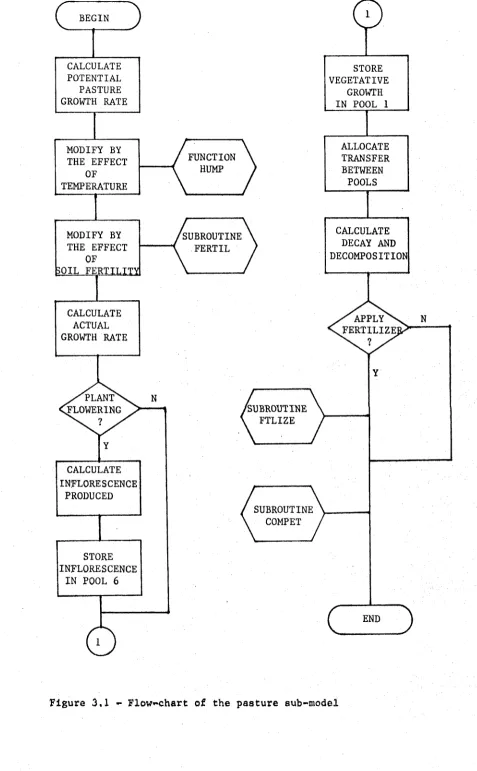
A flow chart of the pasture submodel is shown in Figure

3.1. Growth of each species is considered to be a function

of the amount of photosynthetically active tissue,

environmental variables and soil fertility. The model has

not attempted to consider the separate effects of

/ PLANT'' FLOWERING CALCULATE POTENTIAL PASTURE GROWTH RATE

aOIL FERTILITY MODIFY BY THE EFFECT

OF

CALCULATE ACTUAL GROWTH RATE

CALCULATE INFLORESCENCE

PRODUCED MODIFY BY THE EFFECT

OF TEMPERATURE

STORE INFLORESCENCE

IN POOL 6

FUNCTION HUMP

SUBROUTINE FERTIL

Su b r o u t i n e

FTLIZE

SUBROUTINE COMPET

^ APPLY \

f e r t i l i z e: CALCULATE

DECAY AND DECOMPOSITION

STORE VEGETATIVE

GROWTH IN POOL 1

ALLOCATE TRANSFER BETWEEN

POOLS

nutrients within the plant been incorporated in the model. The four green leaf, sheath and stem pools have been included to allow a representation of ageing within a pasture sward - the pools have no physical counterparts.

It is assumed that elements other than phosphorus (P) and nitrogen (N) are not limiting pasture production although the results of Anderson and Arnot (1953) indicate that this is almost certainly incorrect. Only P and N are considered in the model as the economic and energetic cost of maintaining adequate amounts of most other elements is relatively small. Thus, even if deficiencies of elements other than P and N are widespread, the costs of correcting these deficiencies will probably be low enough to allow the major conclusions of experiments with the model to still apply.

Environmental Effects

Two environmental variables are considered to directly affect plant growth in the model. They are temperature and the ratio of actual to potential evapotranspiration (evaporation ratio). Light can have an effect on plant growth either by virtue of its intensity or its duration (photoperiod) . The effect of varying intensities of radiation on plant growth has not been considered in the model because radiation was considered not likely to limit production in the environment under study (Colman 1971) . The results of Knight (1955) with paspalum suggest that photoperiod changes can influence growth directly and, also, indirectly by the induction of flowering. No direct effect is considered in the model because the unconfounded extraction of such an effect from Knight's data was not possible; however, flower induction has been included.

Effect of temperature

G R O W T H R AT E □

X

CD H fN <

B ’O

CO CO

^ -u

U -H

•H

<

a'D

trö

iro

reached as temperature increases thereby increasing reaction and diffusion rates till finally a critical temperature is reached beyond which the negative effects of an increased rate of enzyme denaturation exceed any increase due to

increased reaction and diffusion rates.

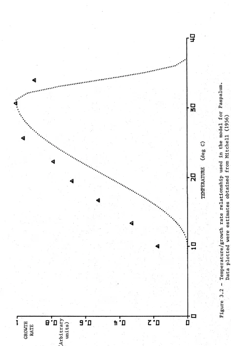
It will be noted that the temperature/growth rate response curve used in the model is ”to the right” of Mitchell’s (1956) observations (Figure 3.2). This displacement was made because the paspalum on the NSW north coast is almost certainly a different and less cold tolerant ecotype than the New Zealand ecotype used in Mitchell's studies. The effects of acclimatization on the development of many species of plants has been recognised for at least a century (Schimper 1903). The derivation of the functions used to define the curve in Figure 3.2 is presented in Appendix B, The curve is defined by three parameters : the

temperature below which no growth occurs, the temperature of maximum growth and the temperature above which no growth occurs.

The parameters used to define the temperature/growth response curves were based on the work of Mitchell (1956) with less emphasis being placed on the less definitive publications of Knight and Bennett (1953), Knight (1955), and Evans, Wardlaw and Williams (1964). The views of research workers familiar with the responses of the species being studied to the north coast environment also influenced the finally selected values.

Table 3.1 - Temperatures used to define temperature/growth rate relationships.

Species Temperature below Temperature of Temperature above which no growth maximum growth which no growth

occurs occurs

Carpet grass 12 31 37

Paspalum 10 31 37

Kikuyu 8 28 34

White clover 0 25 29

Estimated leaf temperature, rather than mean daily temperature, is used in the model to asses the effect of temperature on plant growth rate. Linacre (1964) reviewed the relationship between leaf and air temperatures. Up to about 35 deg, the leaf temperature exceeded the ambient temperature; the relationship between leaf temperature (TEMPLF) and ambient temperature (TEMP) for well watered plants was approximated by

TEMPLF = 9.0 + .74*TEMP

Effect of Transpiration

The method of estimating potential (EVPOT) and actual (EVACT) evapotranspiration has been outlined in the description of the climate generator. From these two variables the evaporation ratio (RATIO) is calculated

RATIO = EVACT/EVPOT

Hence, the evaporation ratio lies in the interval (0,1). Potential plant growth is multiplied by the value of RATIO to define the effect of evaporative demand and soil moisture on plant growth.

De Wit (1958) suggested that plant growth rate was proportional to evaporation ratio. His analysis of data existing at that time from "climates with a large percentage of bright sunshine" supported such an hypothesis; however, data from the Netherlands did not. Although de Wit argued that light intensity had an important influence on the relationship between dry matter production, transpiration and free water evaporation he did not include it in the equation relating these variables. Consequently, the relationships he suggested can in no sense be universal. Despite this, a proportional relationship between growth and evaporation ratio has been assumed in the model. The models of Freer et al. (1970) and Wright (1970) made the same assumption. Vickery and Hedges (1972) defined plant relative growth rate as a function of soil moisture. This function was almost identical to the function relating soil moisture to evaporation ratio, hence Vickery and Hedges virtually assumed that direct proportionality existed between growth rate and evaporation ratio.

E f f e c t o f Amo u n t o f T i s s u e

M e d a w a r ( 1 9 4 1 ) d e f i n e d t h e s e c o n d " l a w " o f b i o l o g i c a l

g r o w t h t o b e " w h a t r e s u l t s f r o m b i o l o g i c a l g r o w t h i s i t s e l f ,

t y p i c a l l y , c a p a b l e o f g r o w i n g " . T h i s t h o u g h t i s i m p l i c i t i n

a l l t h e " g r o w t h e q u a t i o n s " w h i c h h a v e b e e n d e v e l o p e d , i . e .

t h e y c a n a l l b e e x p r e s s e d i n t h e f o r m

d W/ d t = f ( W)

w h e r e d W / d t i s t h e i n s t a n t a n e o u s r a t e o f c h a n g e o f t i s s u e

w e i g h t ( g r o w t h r a t e ) , a n d W r e p r e s e n t s t h e a m o u n t o f t i s s u e

a t a n y o n e t i m e a n d f ( W) i s a f u n c t i o n . Th e b e s t k nown

g r o w t h f u n c t i o n s a r e t h e m o n o m o l e c u l a r , a u t o c a t a l y t i c

( l o g i s t i c ) a n d G o m p e r t z c u r v e s .

P u b l i s h e d w o r k d e s c r i b i n g e i t h e r t h e u s e o r d e v e l o p m e n t

o f g r o w t h f u n c t i o n s g e n e r a l l y f a l l s i n t o o n e o f t wo c l a s s e s .

T h e r e a r e a u t h o r s who s p e a k o f " l a w s " o f a l l o m e t r y a n d g r o w t h

( B e r t a l a n f f y 1 9 5 7 ) , w h i l s t o t h e r s a r e m o r e p r a g m a t i c a n d

s p e a k o f e m p i r i c a l c u r v e s ( R i c h a r d s 1 9 5 9 , 1 9 6 9 ; G o u l d 1 9 6 6 ;

P i e n a a r a n d T u r n b u l l 1 9 7 3 ) . The i n t e r p r e t a t i o n o f W i l l i a m s

( 1 9 6 4 ) i s n e i t h e r i n o n e c l a s s n o r t h e o t h e r . W i l l i a m s

c o m p a r e d t h e r e s u l t s o f f i t t i n g a l o g i s t i c a n d a c u b i c

p o l y n o m i a l t o some w h e a t g r o w t h d a t a . He d e s c r i b e d t h e c u b i c

a s " b e i n g l e s s e x a c t i n g i n t h e a s s u m p t i o n s i t m a k e s " . The

f a c t t h a t W i l l i a m s saw t h e l o g i s t i c i m p o s i n g a s s u m p t i o n s

i m p l i e s h e wa s u s i n g i t i n t h e B e r t a l a n f f y s e n s e a s a c u r v e

w h i c h d e f i n e d a " l a w o f g r o w t h " . On t h e o t h e r h a n d , t h e

s e c o n d c u r v e W i l l i a m s f i t t e d wa s a c u b i c p o l y n o m i a l w h i c h

was c h o s e n a s i t i s a u s e f u l e m p i r i c a l c u r v e l i k e l y t o g i v e a

g o o d d e s c r i p t i o n o f t h e d a t a p o i n t s . T h u s , t h e p h i l o s o p h y

i m p l i c i t i n W i l l i a m s ’ f i t t i n g o f t h e l o g i s t i c c u r v e was

d i a m e t r i c a l l y o p p o s e d t o t h a t u s e d wh e n f i t t i n g t h e c u b i c

p o l y n o m i a l . C o n s e q u e n t l y , t h e l o g i s t i c wa s r e j e c t e d o n a n

i n v a l i d b a s i s . I f a l o g i s t i c a n d a c u b i c p o l y n o m i a l a r e , i n

some s e n s e , t o b e c o m p a r e d , t h e n t h e c o m p a r i s o n i s o n l y v a l i d

i f b o t h a r e r e g a r d e d a s e m p i r i c a l .

R i c h a r d s ( 1 9 5 9 , 1 9 6 9 ) d i s c u s s e d , i n some d e t a i l , t h e

f i t t i n g o f g r o w t h c u r v e s . He p o i n t e d o u t t h a t t h e c u r v e s c a n