An experimental study of model two-dimensional antiferromagnets

An Experimental Study of Model

Two-Dimensional Antiferromagnets

Fiona C. Coomer

MA(Cantab) MSci AMRSC

A thesis presented for the degree of Doctor of Philosophy

The University of Edinburgh

I hereby declare that this thesis is of my own composition. It is all my own work, unless otherwise stated, carried out at the University of Edinburgh between October 2002 and July 2006. It has not been submitted for any other degree or professional qualification.

There is a need to design and synthesise magnetic materials that can be used as models to test our understanding of fundamental magnetic phenomena. Particularly important areas of current interest include the study of systems that model aspects of the magnetic behaviour of the high-Tc superconductors (low-spin Heisenberg

antiferromagnets on a square lattice) and of highly frustrated magnetic systems. A family of layered copper salts, (5CAP)2CuX4, (5CAP = 5-chloro-2-aminopyridine, X = Cl, Br) is a promising model system for the former class of magnet. The ordered magnetic structure of this system has been studied by neutron diffraction, along with (H, T) phase data and appears classical in character; this picture is confirmed by MuSR data, in addition, inelastic neutron scattering gives an indication of the three dimensional nature of the exchange in this system. The jarosite family of minerals, containing kagome lattices of metal ions, commonly Fe3+, are physical realisations of highly frustrated antiferromagnets. The excitation spectra of these materials have been studied using time of flight inelastic neutron scattering. Hydronium iron jarosite appears to behave as a spin liquid to 2 K despite strong antiferromagnetic coupling between homogeneous spin centres, whereas potassium iron jarosite exhibits conventional spin waves for a kagome lattice antiferromagnet, with contributions to the Hamiltonian of either a Dzyaloshinskii-Moriya interaction or crystal field induced single ion anisotropy. SQUID magnetometry measurements made under pressure in order to perturb the system, reveal changes in ordering behaviour in potassium iron jarosite. The mineral volborthite containing a slightly distorted kagome lattice of Cu2+ ions is particularly interesting as it combines both high frustration and low spin (S = ½). This system has been studied using various

relaxation, all of which indicate that the magnetic correlations are highly unconventional. These show that volborthite also possesses strong antiferromagnetic exchange and fluctuations remain significant down to at least 50 mK, despite the build up of short range antiferromagnetic correlations. Experiments looking at ways to minimise the hydrogen content of the various materials studied, to improve the quality of the data from neutron scattering measurements, are also reported.

First of all I would like to thank Andrew for all his help, encouragement and support throughout the course of this PhD, none of this would have been possible without you. Thanks for having patience and believing in me, and for all the input and ideas, whilst also encouraging me to be independent.

A whole host of people have been invaluable when performing the neutron and muon experiments, at the various facilities around the world. Their help has ranged from trying to explain complex physics theories to me, helping with the intricacies of data analysis and attempting to resolve the problems of a hydrogen filled sample to providing light relief during the many hours of counting. The following all deserve a special mention, Georg Ehlers, Björn Fåk, Ralf Feyerherm, Peter Fouquet, Jason Gardner, Thomas Hansen, Paul Henry, Adrian Hillier, James Lord, Garry McIntyre, Des McMorrow, Hannu Mutka, Henrik Rønnow, John Stride, Ross Stewart, Anne Stunault, Jon Taylor and Dirk Visser. In addition, I would like to thank the technical support at each of the facilities, in particular the cryogenic teams for the many hours spent fiddling with dilution fridges.

A number of academic and support staff from the University of Edinburgh have helped with this project, from helping set up apparatus, making measurements to discussions about theory, these include Ronnie Brown, Philip Camp, Lorna Eades, Francesca Fabbiani, Stuart Johnstone, Konstantin Kamenev, Stuart Mains and Gavin Whittaker.

A big thank you to all the members of the Harrison group and the various project students I’ve worked with throughout the course of my PhD; Adrian, Chris, Gaétan, Goran, Keith, Lynne, Marcela, Mark, Phil and Rob, for help with sample prep, being able to bounce ideas off, for putting up with my general chat in the office and for a few great meals.

The work of a PhD does not stop at the door of the lab, therefore I would like to thank those who have helped to put everything in perspective. Those I’ve lived with, in particular, Catherine, Gwen, Richard and Tony, have probably had to put up with more than their fair share of my project’s highs and lows. The 72nd _{Brownies and all at Nicolson Square}

Methodist have helped to provide an escape from the stress of a PhD, and have coped with my frequent trips away, often at short notice. A special mention to all those who have been up for a natter over a drink or dinner, trips to the cinema, beach or hills or just a good run.

Finally, I’d like to thank my family for their support throughout, for understanding the good and bad times, for holidays and for believing I could do it.

1

INTRODUCTION ... 1

1.1 REFERENCES... 4

2

THEORY ... 6

2.1 MAGNETIC MOMENT... 6

2.2 MAGNETIC EXCHANGE... 10

2.3 ANISOTROPY... 14

2.4 SPIN WAVES... 16

2.5 TWO-DIMENSIONAL MAGNETS... 18

2.6 FRUSTRATION... 21

2.7 KAGOME LATTICES... 26

2.8 PERTURBING MAGNETIC SYSTEMS... 28

2.8.1 Dilution ... 29

2.8.2 Pressure ... 29

2.9 REFERENCES... 31

3

EXPERIMENTAL METHODS ... 37

3.1 SQUIDMAGNETOMETRY... 37

3.1.1 Pressure Cell ... 39

3.3 NEUTRON SCATTERING... 47

3.3.1 Neutron Formation ... 49

3.3.2 Elastic Nuclear Scattering... 50

3.3.3 Powder Diffraction... 54

3.3.4 Magnetic Scattering ... 56

3.3.5 Inelastic Neutron Scattering... 58

3.3.6 Polarised Neutron Scattering ... 64

3.3.7 Neutron Spin Echo ... 67

3.4 REFERENCES... 70

4

SQUARE LATTICE ANTIFERROMAGNETS ... 72

4.1 INTRODUCTION... 72

4.1.1 Previous Work... 73

4.2 SYNTHESIS... 75

4.2.1 Synthesis of 2-Amino-5-Chloropyridinium Tetrachlorocuprate Salt ((5CAP)2CuCl4) ... 75

4.2.2 Synthesis of 2-Amino-5-Chloropyridinium Tetrabromocuprate Salt ((5CAP)2CuBr4) ... 76

4.2.3 Partial Deuteration of 5-Chloro-2-Aminopyridine (d3-5CAP) ... 77

4.2.4 Synthesis of Partially Deuterated (5CAP)2CuCl4... 77

4.3 MUON SPIN ROTATION... 78

4.3.1 Experimental ... 78

4.3.2 Results... 80

4.4.1 (d6-5CAP)2CuBr4... 86

4.4.1.1 Experimental... 86

4.4.1.1.1 Magnetic Critical Behaviour ... 88

4.4.1.2 Results ... 88

4.4.1.2.1 Crystal Structure at 10 K... 88

4.4.1.2.2 Magnetic Structure at 1.8 K and Sublattice Magnetisation... 91

4.4.2 (5CAP)2CuCl4... 93

4.4.2.1 Experimental... 93

4.4.2.2 Results ... 96

4.5 INELASTIC NEUTRON SCATTERING... 100

4.5.1 Experimental ... 100

4.5.2 Results... 101

4.6 DISCUSSION... 104

4.7 CONCLUSIONS... 108

4.8 REFERENCES... 111

5

JAROSITES ... 116

5.1 INTRODUCTION... 116

5.2 PREVIOUS WORK... 117

5.2.1 Structure of the Jarosites ... 119

5.3 EXPERIMENTAL... 120

5.3.1 Syntheses and Redeuteration ... 121

5.3.1.1 Synthesis of Anhydrous Iron (III) Sulfate – Fe2(SO4)3... 121

... 122

5.3.1.3 Synthesis of Deuteronium Alunite – (D3O)Al3(SO4)2(OD)6... 122

5.3.1.4 Synthesis of Potassium Iron Jarosite – KFe3(SO4)2(OD)6... 123

5.3.1.5 Synthesis of Deuteronium Iron Jarosite – (D3O)Fe3(SO4)2(OD)6 – Sample 2 . ... 123

5.3.1.6 Redeuteration of Deuteronium Iron Jarosite – (D3O)Fe3(SO4)2(OD)6 (Sample 2) – Sample 3... 124

5.3.1.7 Neutron Diffraction ... 124

5.3.1.7.1 Experimental ... 124

5.3.1.7.2 Results... 125

5.3.2 D.c. Susceptibility Measurements Under Pressure ... 128

5.3.2.1 Experimental... 128

5.3.2.2 Results ... 129

5.3.2.3 Discussion ... 130

5.3.3 Inelastic Neutron Scattering of Potassium Iron Jarosite ... 131

5.3.3.1 IN4 at the ILL... 131

5.3.3.1.1 Experimental ... 132

5.3.3.2 MARI at ISIS... 133

5.3.3.3 Experimental... 134

5.3.3.4 Results ... 135

5.3.3.5 Calculations and Discussion... 141

5.3.3.5.1 Single-ion Anisotropy and the Crystal Field Model ... 143

5.3.3.5.2 Dzyaloshinskii-Moriya Interactions... 145

5.3.4 Inelastic Neutron Scattering of Deuteronium Iron Jarosite ... 148

5.3.4.1 Experimental... 148

5.4 CONCLUSIONS AND FURTHER WORK... 154

5.5 REFERENCES... 157

6

VOLBORTHITE ... 162

6.1 INTRODUCTION... 162

6.2 PREVIOUS STUDIES OF VOLBORTHITE... 163

6.2.1 Structure of Volborthite ... 163

6.2.2 Magnetic Properties ... 165

6.3 EXPERIMENTAL... 168

6.3.1 Syntheses... 169

6.3.1.1 Synthesis of Volborthite, Cu3V2O7(OH)2·2H2O – Sample V1 ... 169

6.3.1.2 Syntheses of Deuterated Volborthite... 169

6.3.2 D.c. Susceptibility of Volborthite ... 170

6.3.2.1 Experimental... 170

6.3.2.2 Results ... 171

6.3.3 MuSR ... 172

6.3.3.1 Experimental... 172

6.3.3.2 Results ... 173

6.3.4 Neutron Spin Echo ... 177

6.3.4.1 Sample Synthesis – Sample V2 ... 179

6.3.4.2 Experimental... 179

6.3.4.3 Results ... 180

6.3.5 XYZ-Polarised Diffuse Neutron Scattering... 181

6.3.5.1 First D7 Experiment ... 183

6.3.5.1.2 Results – Sample V2 ... 183

6.3.5.1.3 Sample Synthesis – Sample V3... 185

6.3.5.1.4 Results – Sample V3 ... 185

6.3.5.1.5 Sample Synthesis – Sample V4... 187

6.3.5.1.6 Results – Sample V4 ... 187

6.3.5.2 Second D7 Experiment... 189

6.3.5.2.1 Sample Synthesis – Sample V5... 189

6.3.5.2.2 Experimental ... 189

6.3.5.2.3 Results... 190

6.3.6 Time of Flight Inelastic Neutron Scattering... 196

6.3.6.1 DCS at NIST... 196

6.3.6.2 IN4 at the ILL... 199

6.3.6.2.1 Sample Syntheses... 200

6.3.6.2.1.1 Synthesis of ‘Deuterated’ Volborthite – Sample V6 200 6.3.6.2.1.2 Synthesis of ‘Deuterated’ Volborthite – Sample V7 201 6.3.6.2.2 Experimental ... 201

6.3.6.2.3 Results... 202

6.3.6.3 MARI at ISIS... 206

6.3.6.3.1 Synthesis of Fully Deuterated Volborthite, Cu3V2O7(OD)2·2D2O – Sample V8 ... 207

6.3.6.3.2 Experimental ... 207

6.3.6.3.3 Results... 209

6.4 DISCUSSION... 212

6.5 CONCLUSIONS AND FURTHER WORK... 215

6.6 REFERENCES... 216

A1.1 CRYSTAL STRUCTURE AT 10K... 219

A1.2 MAGNETIC STRUCTURE AT 1.8K... 220

A1.3 REFERENCES... 224

A2

APPENDIX A2... 225

A2.1 PUBLICATIONS... 225

1 Introduction

Since the discovery of lodestone, a magnetic iron ore, by the Greeks almost 3000 years ago[1], magnetic materials and their properties have been of great interest. Magnetic materials first attracted attention due to their use as navigational aids, but within the past few hundred years, the uses of magnetic materials have greatly expanded, particularly with the discovery of the relationship between electricity and magnetism. Chadwick’s discovery of the neutron in 1932[2], with its magnetic moment, greatly opened up the field of research by providing an incisive probe of magnetism at an atomic and microscopic scale.

Magnetism is of particular interest to the chemist, as the magnetic properties of a material such as the dimensionality, strength of interaction, spin state and any spin anisotropy can often be tuned by altering the structure or chemical composition. Even though the bulk magnetic properties of a material can give an insight into its magnetic behaviour at an atomic level, the direct relationship between the two is not always well understood. As a result, there is a large amount of interest from theoreticians in this area. In order to test and improve their models, theoreticians rely on chemists to produce model magnetic systems. The challenge to the chemist is then to design and synthesise materials containing magnetic structures which correspond to the structures for which theories have been produced, and thus to test these theories[9].

The link between electricity and magnetism is particularly important, as the study of magnetic materials can give insights into the electrical and electronic properties of matter. One such link is between the magnetic fluctuations in low dimensional systems and the behaviour of the high-Tc superconductors. In 1973, Anderson

proposed that a new electronic state may exist as an alternative to the long range ordered Néel state, for low spin systems[3]. This so-called resonating valence bond (RVB) state consists of a fluid of mobile valence bonds (pairs of spins correlated together in singlets), and is favoured by low spin, low dimensionality and the element of frustration. This will be discussed further in chapter 2. It was later proposed by Anderson[4] that the RVB state may contribute to the mechanism of superconductivity in the high-Tc superconductors. In order to further understand

Most of the high-Tc superconductors are based on a structure containing

two-dimensional (2D) layers of S = ½, Cu2+ ions occupying a square lattice[10, 11]. The study of model systems containing lattices of this type, but which do not themselves exhibit superconductivity, enables the magnetic mechanisms present in the high-Tc superconductors to be further understood. One such model system is the

family of copper salts (5-chloro-2-aminopyridine)2CuX4 ((5CAP)2CuX4), where X is a halide ion[12, 13]. The static and dynamic behaviour of these compounds have been studied in more depth in this thesis, including looking at the effect of perturbing such systems by the application of a field or doping the lattice, and details of such experiments can be found in chapter 4.

Many different materials with the jarosite structure have been synthesised, but to date there are no examples containing S = ½ ions on the kagome lattice sites. In order to maximise the chance of an exotic ground state, the factors of low spin, low dimensionality and frustration should all be combined, and the case of a magnet consisting of S = ½ ions on the kagome lattice possesses all of these factors. One such material is the mineral volborthite, containing Cu2+ ions on slightly distorted kagome layers[17]. Further details of a variety of experiments performed on this system to probe both the static and dynamic behaviour can be found in chapter 6.

This thesis contains details of how the aforementioned model magnetic systems have been synthesised, perturbed and measured using a variety of techniques. The techniques used to probe the behaviour of these systems include SQUID magnetometry, muon spin relaxation and both elastic and inelastic neutron scattering. Further details of the experimental techniques used throughout the course of this project can be found in chapter 3.

1.1 References

[1] Blundell, S. J., Magnetism in Condensed Matter. Oxford Master Series in Condensed Matter Physics, ed. 2001, (Oxford University Press: New York). [2] Chadwick, J., Nature, 1932, 129: 312.

[3] Anderson, P. W., Mat. Res. Bull., 1973, 8(2): 153-160. [4] Anderson, P. W., Science, 1987, 235(4793): 1196-1198.

[6] Mydosh, J. A., Spin Glasses: An Experimental Introduction, ed. 1993, (Taylor & Francis: London - Washington DC).

[7] Bramwell, S. T. and Harris, M. J., J. Phys.: Condens. Matter, 1998, 10: L215 - L220.

[8] Ramirez, A. P., Hayashi, A., Cava, R. J., Siddharthan, R. and Shastry, B. S., Nature, 1999, 399(6734): 333-335.

[9] Harrison, A., J. Phys.: Condens. Matter, 2004, 16: S553-S572.

[10] Kastner, M. A., Birgenau, R. J., Shirane, G. and Endoh, Y., Rev. Mod. Phys., 1998, 70(3): 897-928.

[11] Manousakis, E., Rev. Mod. Phys., 1991, 61: 1-62.

[12] Woodward, F. M., Albrecht, A. S., Wynn, C. M., Landee, C. P. and Turnbull, M. M., Phys. Rev. B, 2002, 65(14): art. no.-144412.

[13] Hammar, P. R., Dender, D. C., Reich, D. H., Albrecht, A. S. and Landee, C. P., J. Appl. Phys., 1997, 81(8): 4615-4617.

[14] Ramirez, A. P., Annu. Rev. Mater. Sci., 1994, 24: 453-480. [15] Greedan, J. E., J. Mater. Chem., 2001, 11: 37-53.

[16] Hendricks, S. B., Am. Mineral., 1937, 22: 773-784.

2 Theory

2.1 Magnetic Moment

The bulk magnetic properties of a material arise from the magnetic field created on an atomic scale. When a current flows around a loop of wire, the movement of the charge creates a magnetic field. On an atomic scale, the movement of an electron spin about the nucleus creates this effect. According to the Pauli Exclusion Principle, if two electrons occupy the same orbital, they must be of opposite spin. In this case the spins cancel each other out, resulting in no net magnetic field. The magnetic field on an atomic scale is therefore created by the motion of unpaired electrons about a nucleus, resulting in a magnetic moment on the atom. This is termed paramagnetism. In addition, all elements exhibit a degree of diamagnetism; a weak, negative magnetic susceptibility, which causes a moment to be induced that opposes any applied field. This effect is quantum mechanical and will not be discussed further here, as the effect is generally on a much smaller scale than any paramagnetism.

The size of the paramagnetic moment is determined by the total angular momentum (J) of the unpaired electrons, which is composed of spin (S) and orbital (L) components. When S and L can be coupled together by Russell-Saunders coupling to give J, the magnitude of the moment, μJ, is given by the equation:

( 1

J gJ B J J

where μB is the Bohr magneton (= B eħ/2me) and gJ is the Landé g factor:

3 ( 1) ( 1

2 2 ( 1)

J

S S L L

g

J J

)

+ − +

= +

+ . (2.2)

In the case of many transition metal ions, the ligand field has the effect of removing the degeneracy of the singly occupied orbitals; thereby quenching the orbital angular momentum[1]. In this case S can be equated to J, resulting in a ‘spin-only’ moment.

When a magnetic field is applied to an isolated paramagnetic ion, Zeeman splitting occurs. This has the effect of splitting the ground state into (2J + 1) mJ substates,

which have quantised projections along the direction of the applied field, and have energies, Em_J :

J

m J B

E = −m gμ H. (2.3)

At finite temperatures, the population of these states is governed by the Boltzmann distribution. The net polarisation,

J

m

μ of the ion is therefore given by the average over all these states:

exp( / )

exp( / )

j j j J j j J m m m J m J m m J E kT E kT μ μ =− =− − = −

∑

If is small in comparison with the thermal energy, kT, the occupation of each energy level will be approximately the same and the net magnetic polarisation per ion simplifies to:

J

m

E

2 2

0 ( 1

3 J

B m

g B J J kT μ

μ = + ), (2.5)

where BB0 is the magnetic flux in a vacuum. For one mole of ions, the total magnetisation, M, is equal to NA μ_mJ . Experimentally, the quantity that is

determined is the susceptibility, χ, which is defined as the ratio of M to the applied field (H):

M C

H T

χ= = , (2.6)

where:

2 2 _{( 1}

3 A B

N g J J C

k

μ + )

= . (2.7)

C is known as the Curie constant, and this behaviour of the susceptibility is known as the Curie law. Measurement of C enables the size of the magnetic moment on individual ions to be calculated. The Curie law only applies for the perfect paramagnet – when there is no interaction between magnetic moments; a system analogous to an ideal gas.

CW

C T χ

θ

=

− , (2.8)

where θCW is known as the Weiss constant. The magnitude of θCW is governed by the

strength of the internal field experienced by each ion, i.e. the strength of the interaction between magnetic ions. If θCW is positive, this indicates that there is a

tendency towards a local parallel alignment of spins on neighbouring ions, which is known as ferromagnetism. Similarly, if θCW is negative, the local alignment of spins

on neighbouring ions is predominantly antiparallel; this is known as antiferromagnetism.

In order to quantify both C and θCW, the susceptibility of a sample is measured as a

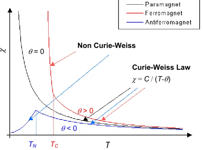
long range ordered state, known as the Néel state, can be thought of as consisting of two sub-lattices of moments aligned in a parallel fashion. The susceptibility plotted as a function of temperature for perfectly paramagnetic, ferromagnetic and antiferromagnetic materials is shown in figure 2.1.

Figure 2.1: Graphs of susceptibility (χ) vs. temperature (T) for an ideal paramagnet, antiferromagnet and ferromagnet.

2.2 Magnetic Exchange

Within a solid, the magnetic moments on different atoms may interact, resulting in deviations from the behaviour exhibited by a perfect paramagnet. The alignment between spins on neighbouring ions can arise through a number of different mechanisms, but is generally termed magnetic exchange. A spin Hamiltonian can be written down to describe the energy of the exchange between two magnetic species:

2

ij = − Jij i⋅ j

H S S , (2.9)

χ

θ <0

Non Curie-Weiss

Curie-Weiss Law

χ = C / (T-θ

θ >0

T

)

where J is the exchange parameter describing both the magnitude and the type of interaction between the two spins at sites i and j. As it involves a scalar product of the two spin vectors, the Hamiltonian is minimised when the two spins are aligned in a co-linear fashion. A positive value of J describes ferromagnetic exchange, and a negative value, antiferromagnetic exchange.

The most obvious interaction that might be expected to play a part in the exchange between magnetic ions is the magnetic dipolar interaction, which is a through-space interaction. The order of magnitude of this effect is so small that it only becomes important over very short ranges or at very low temperatures (< 1 K for two moments of 1 μB, a distance of 1 Å apart). This type of interaction therefore does not account

for the magnetic exchange in most compounds.

B

In a conductor, the conduction electrons can mediate the exchange interaction between ions. This effect is known as the RKKY mechanism, after its discoverers Ruderman, Kittel, Kasuya and Yosida. The magnetic moment on an ion spin-polarises the conduction electrons, which then couple to another moment a distance away. This type of interaction is long range, and the sign of the coupling has an oscillatory dependence upon the distance between the moments.

the overlap becomes greater, the Pauli Exclusion Principle comes into play, forbidding the two electrons from having the same spin, thus stabilising the singlet state. Therefore the spins align in an antiparallel fashion (antiferromagnetic exchange), and as the overlap becomes greater, a bond is formed. Direct exchange is not common; as metal ions are rarely close enough in an insulator for direct interactions to occur, although it may come into play for systems containing edge or face sharing MO6 octahedra.

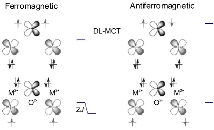
The most common way in which magnetic exchange occurs in an insulator is via the orbitals on an intermediate diamagnetic atom or atoms. This is known as superexchange[2]. Kinetic superexchange stabilises the antiferromagnetic ground state through the overlap of two half-filled d-orbitals (eg for the σ case and t2g for the

Ferromagnetic Antiferromagnetic

2J

DL-MCT

M-MCT

M2+ _O

2-M2+ _M2+ _O

2-M2+

Figure 2.2: Orbital pathways for kinetic superexchange via a σ-type interaction through a ligand p orbital.

Ferromagnetic Antiferromagnetic

2J

DL-MCT

M2+

O

2-M2+

M2+

O

2-M2+

Figure 2.3: Orbital pathways for potential superexchange via a σ-type interaction, through orthogonal orbitals (ligand px and py).

The dominant pathway is almost always the kinetic superexchange pathway and therefore antiferromagnetic exchange dominates. The exception to this is when the metal – ligand – metal bridging angle through the ligand is close to 90º. This leads to ferromagnetic exchange being dominant. The size of the exchange is very sensitive to the degree of orbital overlap; therefore the type of bonding (e.g. σ or π), the bond angle and the ionic radius are important factors in determining the nature of the exchange.

2.3 Anisotropy

2 z z ( x x y y i j i j i j i j

J a b

>

)

⎡ ⎤

= −

∑

H S S S S S S . (2.10)

In the case when a = b = 1, the system is fully isotropic, and therefore the spin is free to align, without preference, in any orientation. This is known as the Heisenberg case. If a = 0 and b = 1, the moment is confined to lie in the xy-plane, known in this case as the easy plane; this is known as the XY case. Similarly, if a = 1 and b = 0, the moment is confined to lie along the z-axis (easy axis), which corresponds to the Ising case. The degree of anisotropy is influenced mainly by the crystal field that the magnetic ion experiences. The crystal field, through spin-orbit coupling, provides a preferred direction of alignment. Also, asymmetry in the available exchange pathways will lead to anisotropic interactions and therefore a preferred alignment direction.

Another interaction that can lead to anisotropy is the Dzyaloshinskii-Moriya (DM) interaction[4, 5]. This interaction is between an excited state of one ion and the ground state of another, and leads to an additional term in the Hamiltonian:

[

]

⋅ ×

D S S . (2.11)

plane perpendicular to D). This has the effect of causing the moments to cant by a small angle, leading to so called Dzyaloshinskii-Moriya ferromagnetism.

The degree of anisotropy in the system, expressed by the parameter D, along with the dimensionality of the system, d, governs the range of magnetic order that can occur in the solid. This is shown in table 2.1:

One-dimensional

d = 1 Two-dimensional d = 2 Three-dimensional d = 3 Ising

D = 1

Short range order Long range order Long range order XY

D = 2

Short range order Medium range order Long range order Heisenberg

D = 3 Short range order Short range order Long range order

Table 2.1: Effects of anisotropy and lattice dimensionality on the range of any magnetic ordering.

In reality, a system is rarely ideal, and is usually a mixture of some of the above cases. This is due to the difficulty in eliminating longer range interactions from the system, and the fact that the spin anisotropy rarely conforms exactly to one of the above situations. As can be seen from table 2.1, two-dimensional systems are particularly interesting as the range of their ordering is dependent upon the anisotropy of the moment. The work in this thesis concentrates on various types of approximately two-dimensional systems.

2.4 Spin Waves

quite the case). At finite temperatures, the thermal energy has the effect of disrupting this order by creating lattice vibrations. These vibrations are quantised as phonons. The magnetic analogy of these lattice vibrations are spin waves, which are quantised as magnons. If we consider a linear chain, at T = 0, the magnetic moments on each of the ions will be aligned; for a ferromagnet, in a parallel manner, and in an antiparallel manner for an antiferromagnet, with the precession of the moments all being perfectly in phase. At finite temperatures, thermal fluctuations cause the precession of adjacent moments to be out of phase with respect to their neighbours by a constant amount, ka, where k is a quantum number known as the wavenumber and a is the lattice constant. This results in a spin wave of wavelength 2π/k.

Figure 2.4: Classical picture of a spin wave in a linear ferromagnetic chain of n spins, with a lattice constant a. The arrows represent the spins precessing about the internal field. Figure taken from reference[6].

dispersion relation. It can be shown[7] that for a ferromagnetic chain, the dispersion relation is of the form:

4JS(1 coska)

ω= −

= . (2.12)

Additional terms in the Hamiltonian, such as spin anisotropy, or additional interactions, will modify the dispersion relation, but by measuring the dispersion, J can often be calculated.

2.5 Two-Dimensional Magnets

or

₊

₊

…

= ( - )

Figure 2.5: The Néel and RVB ground states in a 2D square Heisenberg antiferromagnet. Each bold line represents an antisymmetrised singlet.

The 2D Heisenberg model on a square lattice is particularly important as, for the low spin (quantum) case, it pertains to the behaviour of the high-Tc cuprate superconductors[9, 11, 12]. The high-Tc cuprate superconductors, such as BaxLa5-xCu5O5(3-y), YBa2Cu3O7-y and HgBa2Ca2Cu3O8+y contain square lattices of

S = ½, Cu2+ ions exhibiting Heisenberg spin symmetry. Due to the potential applications of this kind of system, there has been a large amount of theoretical interest. It is found theoretically that on lowering the temperature, there is no onset of long range order at finite temperatures, but there is an increase in the size of the areas of short-range order – increasing the correlation length, ξ. The correlation length diverges exponentially with 1/T, until long range order is established at T = 0[12]. These systems would be expected to behave in a classical manner, and this is observed in terms of their ground state, but experimentally quantum fluctuations may lead to non-classical behaviour particularly in terms of the one-magnon spectrum[13, 14] and behaviour in high applied magnetic fields[15]. Quantum effects lead to non-linear spin wave behaviour near the zone boundary of the one-magnon dispersion, hinting at the existence of RVB-type fluctuations. In fields close to the saturation field, Hs (= 4J), the spin waves should become unstable

In order to study the behaviour of the 2D Heisenberg model, good model systems are needed. A good model for a two-dimensional system will have well separated layers, typically with a ratio of intraplane to interplane coupling J/J’ ≥ 100. High-Tc

superconductors are themselves poor model systems, due to their poor crystallinity, the difficulty in obtaining samples of the precise composition required, and the strong magnetic coupling within these systems which results in an energy scale too high to be experimentally probed. One good model system is copper formate tetradeuterate (CFTD)[16]. This system obeys theory very well, as it has a Hamiltonian close to that expected for the 2D square Heisenberg antiferromagnet, and it has been studied in some detail [13, 16-22]. As the stability of this system is finely balanced, it is often desirable to perturb it in some way (see section 2.8). Unfortunately, due to the size of the coupling in this system (J = 72 K), the magnetic fields required to saturate this system are beyond reach experimentally (Hc = 250 T).

Also, it has not been possible to dope this system to a significant level.

2.6 Frustration

The collective properties of a magnetic system may also be affected by frustration. Magnetic frustration is a term that describes the situation in which the magnetic sites on a lattice are subject to competing or contradictory constraints. When this arises from the topology of the lattice, it is termed geometrical frustration. To illustrate this concept, consider a square arrangement of spins (figure 2.6(a)), where only the nearest neighbour interactions are in operation; if the exchange is antiferromagnetic, all the spins can align in their preferred orientation, satisfying all the interactions. On the other hand, for a triangular arrangement of spins (figure 2.6(b)), with three equal antiferromagnetic interactions, only two of the interactions can be simultaneously satisfied. There is no minimisation of all the exchange terms, resulting in one frustrated spin. Similarly for a square arrangement with one ferromagnetic and three antiferromagnetic interactions (figure 2.6(c)), only three of these interactions can be satisfied simultaneously, leaving one frustrated spin.

?

?

FM

AFM AFM

(a) (b) (c)

Figure 2.6: (a) A square arrangement of antiferromagnetically coupled spins, (b) frustration on an equilateral triangle, (c) frustration on a square due to one ferromagnetic interaction. In (b) & (c) the red spin is frustrated.

triangular lattice of edge sharing equilateral triangles and the kagome lattice of corner sharing equilateral triangles. In three dimensions possible frustrated lattices include the pyrochlore structure of corner sharing tetrahedra and the face centred cubic (FCC) lattice of edge sharing tetrahedra.

(a) (b)

(c) (d)

Figure 2.7: (a) Triangular, (b) kagome, (c) pyrochlore and (d) face centred cubic lattices.

will occur at the Curie-Weiss temperature, θCW, i.e. TN = θCW. As the degree of

frustration in the system increases, the ordering temperature decreases in relation to

θCW. The degree of frustration, f, is therefore defined as[30]:

CW N

f T θ

= . (2.13)

For a ferromagnet, f is close to 1, but for a non-frustrated antiferromagnet, f is often greater than 1 and can be as large as 4 or 5[31]. For a truly frustrated system, f is usually larger than 10 and can be even greater than 500[32].

In many cases, when the spins exhibit either Heisenberg or XY anisotropy, a compromise spin arrangement of minimum energy is adopted around the plaquette. For the case of the triangular motif, the compromise configuration is the 120º arrangement shown in figure 2.8. In this case, there are two possible compromise configurations; each has a different chirality depending on whether the spins rotate in a clockwise or anticlockwise direction on going around the triangle in a clockwise manner.

If two triangles are joined together in an edge-sharing fashion, the spin configuration on one triangle unambiguously determines the orientation of the spins on the next triangle (see figure 2.9(a)), and any chiral information is passed on. On the contrary, if the triangles are joined together by their corners, the spin configuration around the first triangle allows two possible minimum energy configurations on the second triangle, each of opposite chirality. In this case, the chiral information is not passed on.

(a) (b) (c)

Figure 2.9: (a) Edge sharing triangles showing the unique orientation of the red spin in order to satisfy the 120° minimum energy configuration, (b) & (c) corner sharing triangles showing the two possible orientations of the red spins satisfying the 120° minimum energy configuration.

but a number of degenerate ground states of the spin structure. Two of these states that exhibit long range order are the so-called ‘q = 0’ and ‘√3 x √3’ structures.

(a) (b) (c)

Figure 2.10: 120º compromise arrangements on lattices: (a) triangular lattice, (b) q = 0 arrangement on the kagome lattice and (c) √3 x √3 arrangement on the kagome lattice.

Similarly, in three dimensions, the pyrochlore lattice of corner sharing tetrahedra, shows no unique ground state, unlike the FCC lattice.

A consequence of the competing interactions in a frustrated lattice is that these materials often do not exhibit long range order, but more exotic ground states may be observed. These may include spin glasses, spin ices and spin liquids. A spin glass is a state in which the spins are frozen into a pattern not exhibiting any long-range order. There is a distinct freezing temperature at which this occurs, known as the glass transition temperature, Tg. Below this temperature one of many degenerate

susceptibility and a strong slowing down of the spin dynamics below Tg, but an

absence of long range order. A spin liquid is a system in which the spins remain dynamic down to the lowest temperatures, despite correlations between spins. Spin liquids are often referred to in the case of quantum (S = ½) systems, where the RVB ground state may be important. A spin ice is a state that may be formed from Ising spins on the pyrochlore lattice[33, 34], where the spin orientations are analogous to the proton arrangements around the oxygen atoms in ice[35].

In order to study the properties of frustrated lattices, suitable model systems must be found[36]. There are many different approaches to this problem. The first is to look for examples of materials already in existence, these may include naturally occurring minerals or materials previously synthesised. A second approach is to hope that a suitable sample may be produced serendipitously – but this can be very time consuming, with no guaranteed results. A third option is to try and design a material, often based on building up a material from smaller ‘building units’, of the required topology, or by modifying the structure of an existing material, by adding vacancies or interstitials.

2.7 Kagome Lattices

A kagome lattice with classical Heisenberg spins will have a large number of degenerate ground states if only nearest neighbour exchange is considered[37]. It is found that this degeneracy can be lifted by considering any small perturbation, e.g. next-nearest neighbour interactions, anisotropy and structural distortions. Even for the Heisenberg case, it has been shown that the ground state will consist of a planar arrangement of spins, due to the effects of thermal fluctuations[38, 39]. Calculations have shown that thermal fluctuations remove the degeneracy of the ground state, and in the Heisenberg case, the √3 x √3 structure is adopted[40] when only nearest neighbour interactions are considered. When further neighbour interactions are considered, the degeneracy of the ground state is either partially or fully lifted[41] depending on the nature of the interaction.

Despite the large amount of theoretical work concentrated on the kagome lattice, there are very few physical representations of the lattice with which to test the theory. Two families of minerals containing metal atoms arranged in kagome lattices have been studied and will be discussed later in this thesis. The jarosite[42] family of minerals contain perfect kagome planes of metal atoms and will be discussed further in chapter 5. The mineral volborthite[43] contains a planar lattice of copper atoms in a slightly distorted kagome arrangement, and will be discussed in chapter 6.

interleaved with triangular lattices. The occupation of the kagome lattice is less than 100 %, and the distortion of the co-ordination octahedra about the Cr atoms, leads to magnetic exchange anisotropy. These factors all mean that, although SCGO is a highly frustrated system[44], exhibiting spin glass behaviour, it is not an accurate model of the kagome lattice[45]. The related material Ba2Sn2ZnGa3Cr7O22 (BSZGCO)[46] does not contain magnetic ions in the intermediary layers that are present in SCGO, making this compound more 2D in character, resulting in a higher degree of frustration. Recently synthesised systems, which could provide a good starting point for further investigation include the mineral herbertsmithite[47] containing kagome layers of S = ½ Cu2+ ions separated by layers containing diamagnetic Zn. To date, there is no evidence of long range ordering in this system. There are a few examples of materials containing kagome lattices of metals templated by organic ligands, these include the S = 1, Ni2+ containing compound [C6N2H8][NH4]2[Ni3F6(SO4)2] [48], and the S = ½ compound {Cu3(titmb)2(OCOCH3)6}·H2O (titmb = 1,3,5-tris (imidazol-1-ylmethyl)-2,4,6-trimethylbenzene)[49]. These materials both present a problem with making samples suitable for study by neutron scattering techniques, due to the difficulty and expense associated with producing perdeuterated samples.

2.8 Perturbing Magnetic Systems

delicately balanced. There are many ways of perturbing a system, the most commonly used ways being the variation of temperature and applied magnetic field. Other ways of perturbing a system can include making systematic structural changes (e.g. changing the ionic radius of a counter ion), doping the magnetic lattice with diamagnetic ions or applying pressure to the system.

2.8.1 Dilution

Doping the magnetic lattice with diamagnetic ions (or diamagnetic dilution) has the effect of randomly introducing site vacancies in the lattice. Dilution is usually carried out with a diamagnetic element possessing a similar size and chemical properties to the paramagnetic ion. This minimises distortion of the lattice, and ensures that the doping is random in nature. If the level of dilution is great enough, the exchange pathways across the lattice will be broken, preventing long-range order. This will occur at the percolation threshold pc[50]. Up to this point, the range of

ordering will be affected by the level of dilution, as will the transition temperature. By altering the level of doping, these properties can be tuned.

2.8.2 Pressure

may therefore result in the alteration of the magnetic interactions. Structural distortions are often introduced into a material by altering the ionic radius of one or more of the components, by replacement with another (this is often referred to as ‘chemical pressure’). This technique is not always satisfactory as the replacement may cause a completely different structure or compound to form. Also, the structural distortions can only be created in discrete steps (depending on the radii of the ions available), rather than being varied continuously. There are therefore many advantages in introducing structural distortions by the application of pressure; structural distortions can be introduced in a continuous manner to a sample of known structure and magnetic properties, without the need to synthesise a new compound, and all the problems associated with that. Applying pressure to a system, and measuring the corresponding structural and magnetic changes should increase our knowledge of the mechanisms leading to and affecting magnetic exchange.

Considering the obvious information that can be obtained by looking at the effects of pressure on the structural and magnetic properties of a system, remarkably little work has been carried out in this field. Most of the work done to date has been concerned with the study of pressure on the magnetic properties of alloys. Early work on magnetic insulators investigated the pressure dependence of both structural and magnetic properties, resulting in a relationship between the strength of the superexchange, J, and the distance between the magnetic moments, r[51-55]:

n

where n is ~ 10. More recent studies have involved using pressure as another tool to probe materials that are of current interest in solid state magnetism. These include materials related to the high-Tc superconductors[56, 57], colossal

magnetoresistors[58-60], and other materials where the effect of pressure on the Jahn-Teller distortion may affect the magnetic ordering[61-64]. The effect of pressure on frustrated systems has also been investigated. One such system is the pyrochlore lattice spin liquid, Tb2Ti2O7[65, 66]. The application of pressure to this system induces long range magnetic order, and it has been found that the Néel temperature and ordered magnetic moment may be tuned by the direction of any anisotropic pressure component.

2.9 References

[1] Carlin, R. L., Magnetochemistry, ed. 1986, (Springer-Verlag: Berlin). [2] Anderson, P. W., Phys. Rev., 1950, 79(2): 350 - 356.

[3] de Jongh, L. J. and Miedema, A. R., Advances in Physics, 1974, 23(1): 1-247. [4] Dzyaloshinsky, I., J. Phys. Chem. Solids, 1958, 4(4): 241 - 255.

[5] Moriya, T., Phys. Rev., 1960, 120(1): 91 - 98.

[6] Wills, A. S., PhD Thesis. 1996, University of Edinburgh.

[7] Blundell, S. J., Magnetism in Condensed Matter. Oxford Master Series in Condensed Matter Physics, ed. 2001, (Oxford University Press: New York). [8] Mermin, N. D. and Wagner, H., Phys. Rev. Lett., 1966, 17(22): 1133-1136. [9] Manousakis, E., Rev. Mod. Phys., 1991, 61: 1-62.

[12] Kastner, M. A., Birgenau, R. J., Shirane, G. and Endoh, Y., Rev. Mod. Phys., 1998, 70(3): 897-928.

[13] Rønnow, H. M., McMorrow, D. F., Coldea, R., Harrison, A., Youngson, I. D., Perring, T. G. et al., Phys. Rev. Lett., 2001, 87(3): art. no.-037202.

[14] Kim, Y. J., Aharony, A., Birgenau, R. J., Chou, F. C., Entin-Wohlman, O., Erwin, R. W. et al., Phys. Rev. Lett., 1999, 83(4): 852 - 855.

[15] Zhitomirsky, M. E. and Chernyshev, A. L., Phys. Rev. Lett., 1999, 82(22): 4536-4539.

[16] Clarke, S. J., DPhil Thesis. 1994, University of Oxford.

[17] Harrison, A., Clarke, S. J., Mason, T. E. and Visser, D., J. Magn. Magn. Mater., 1992, 104: 557-558.

[18] Rønnow, H. M., McMorrow, D. F., Harrison, A., Youngson, I. D., Coldea, R., Perring, T. G. et al., J. Magn. Magn. Mater., 2001, 236(1-2): 4-5. [19] Clarke, S. J., Harrison, A., Mason, T. E. and Visser, D., Solid State Commun.,

1999, 112(10): 561-564.

[20] Rønnow, H. M., McMorrow, D. F. and Harrison, A., Phys. Rev. Lett., 1999, 82(15): 3152-3155.

[21] Clarke, S. J. and Harrison, A., J. Magn. Magn. Mater., 1995, 140: 1627-1628. [22] Clarke, S. J. and Harrison, A., J. Phys.-Condes. Matter, 1992, 4(29):

6217-6226.

[24] Hammar, P. R., Dender, D. C., Reich, D. H., Albrecht, A. S. and Landee, C. P., J. Appl. Phys., 1997, 81(8): 4615-4617.

[25] Matsumoto, T., Miyazaki, Y., Albrecht, A. S., Landee, C. P., Turnbull, M. M. and Sorai, M., J. Phys. Chem. B, 2000, 104(43): 9993-10000.

[26] Place, H. and Willett, R. D., Acta Crystallogr. Sect. C-Cryst. Struct. Commun., 1987, 43: 1050-1053.

[27] Woodward, F. M., Albrecht, A. S., Wynn, C. M., Landee, C. P. and Turnbull, M. M., Phys. Rev. B, 2002, 65(14): art. no.-144412.

[28] Woodward, F. M., Landee, C. P., Giantsidis, J., Turnbull, M. M. and Richardson, C., Inorg. Chim. Acta, 2001, 324(1-2): 324-330.

[29] Woodward, F. M., Albrecht, A. S., Wynn, C. M., Landee, C. P. and Turnbull, M. M., cond-mat, 2001: 0107483.

[30] Ramirez, A. P., Annu. Rev. Mater. Sci., 1994, 24: 453-480. [31] Greedan, J. E., J. Mater. Chem., 2001, 11: 37-53.

[32] Hirakawa, K., Kadowaki, H. and Ubukoshi, K., J. Phys. Soc. Jpn., 1985, 54(9): 3526-3536.

[33] Bramwell, S. T. and Harris, M. J., J. Phys.: Condens. Matter, 1998, 10: L215 - L220.

[34] Ramirez, A. P., Hayashi, A., Cava, R. J., Siddharthan, R. and Shastry, B. S., Nature, 1999, 399(6734): 333-335.

[35] Pauling, L., The Nature of the Chemical Bond, 3rd ed, ed. 1960, (Cornell University Press: Ithaca, NY). pp. 465 - 468.

[38] Chalker, J. T., Holdsworth, P. C. W. and Shender, E. F., Phys. Rev. Lett., 1992, 68(6): 855-858.

[39] Shender, E. F., Cherepanov, V. B., Holdsworth, P. C. W. and Berlinsky, A. J., Phys. Rev. Lett., 1993, 70(24): 3812-3815.

[40] Harris, A. B., Kallin, C. and Berlinsky, A. J., Phys. Rev. B, 1992, 45(6): 2899-2919.

[41] Ballou, R., Canals, B., Elhajal, M., Lacroix, C. and Wills, A. S., Phys. Stat. Sol. (b), 2003, 236(2): 240-245.

[42] Hendricks, S. B., Am. Mineral., 1937, 22: 773-784.

[43] Lafontaine, M. A., Lebail, A. and Ferey, G., J. Solid State Chem., 1990, 85(2): 220-227.

[44] Ramirez, A. P., Espinosa, G. P. and Cooper, A. S., Phys. Rev. Lett., 1990, 64(17): 2070-2073.

[45] Lee, S. H., Broholm, C., Aeppli, G., Perring, T. G., Hessen, B. and Taylor, A., Phys. Rev. Lett., 1996, 76(23): 4424-4427.

[46] Hagemann, I. S., Huang, Q., Gao, X. P. A., Ramirez, A. P. and Cava, R. J., Phys. Rev. Lett., 2001, 86(5): 894-897.

[47] Shores, M. P., Nytko, E. A., Bartlett, B. M. and Nocera, D. G., J. Am. Chem. Soc., 2005, 127: 13462-3.

[48] Behera, J. N. and Rao, C. N. R., J. Am. Chem. Soc., 2006, 128(29): 9334-9335.

[50] Collins, M. F., Magnetic Critical Scattering. Oxford Series on Neutron Scattering in Condensed Matter, ed. 1989, (Oxford University Press: New York).

[51] Bloch, D., J. Phys. Chem. Solids, 1966, 27(5): 881. [52] Bloch, D., Ann. Phys., 1966, 1(1-2): 93.

[53] Bloch, D., Chaisse, F. and Pauthene.R, J. Appl. Phys., 1966, 37(3): 1401. [54] Bloch, D. and Vettier, C., J. Magn. Magn. Mater., 1980, 15-8(JAN-):

589-592.

[55] de Jongh, L. J. and Block, R., Physica B & C, 1975, 79(6): 568-593.

[56] Aronson, M. C., Dierker, S. B., Dennis, B. S., Cheong, S. W. and Fisk, Z., Phys. Rev. B, 1991, 44(9): 4657-4660.

[57] Doroshev, V., Krivoruchko, V., Savosta, M., Shestakov, A. and Tarasenko, T., J. Magn. Magn. Mater., 1996, 158: 669-670.

[58] Moritomo, Y., Kuwahara, H., Tomioka, Y. and Tokura, Y., Phys. Rev. B, 1997, 55(12): 7549-7556.

[59] Imada, M., Fujimori, A. and Tokura, Y., Rev. Mod. Phys., 1998, 70(4): 1039-1263.

[60] Kamenev, K. V., Lees, M. R., Balakrishnan, G., Paul, D. M., Marshall, W. G., Tissen, V. G. et al., Phys. Rev. Lett., 2000, 84(12): 2710-2713.

[61] Ishizuka, M., Terai, M., Endo, S., Hidaka, M., Yamada, I. and Shimomura, O., J. Magn. Magn. Mater., 1998, 177: 725-726.

[63] Ishizuka, M., Yamada, I., Amaya, K. and Endo, S., J. Phys. Soc. Jpn., 1996, 65(7): 1927-1929.

[64] Manaka, H., Yamada, I., Kitazawa, T., Kobayashi, M., Ishizuka, M. and Endo, S., J. Phys. Soc. Jpn., 1997, 66(10): 2989-2992.

[65] Mirebeau, I., Goncharenko, I. N., Cadavez-Peres, P., Bramwell, S. T., Gingras, M. J. P. and Gardner, J. S., Nature, 2002, 420: 54-57.

3 Experimental Methods

This chapter contains details of a number of the experimental techniques used to study both the static and the dynamic nature of any magnetism in a sample, along with techniques that can also be used to gain information about the structure of materials.

3.1 SQUID Magnetometry

In order to measure the magnetic susceptibility (χ) of a material, a known magnetic field (H) needs to be applied to a sample, and the magnetisation (M) measured. One of the most sensitive ways of doing this is to use a Superconducting QUantum Interference Device (SQUID) magnetometer[1]. The SQUID itself consists of a superconducting loop containing two Josephson junctions in the loop’s current path. A Josephson junction is a device based on an electron tunnelling effect and consists of a thin layer of insulating material in a superconducting circuit. This allows the direct observation of quantum electrodynamic phenomena.

junctions. The addition of this to the unaltered wavefunction tunnelling through the other junction creates an interference pattern, which is very sensitive to the magnetic field. As a closed superconducting loop is formed by the detection coils, connecting wires and the SQUID input coil, the change of magnetic flux in the detection coils produces a change in the current in the detection circuit, which is proportional to the change in magnetic flux. The changes in current in the detection coils create variations in the output voltage of the SQUID coil, which are proportional to the magnetic moment of the sample. During a scan, the sample position is varied, in order to alter this output voltage. The output voltage measured as a function of the sample position is then fitted to a theoretical expression in order to give a value of the sample magnetisation[2]. Ideally, the sample will therefore be a point source in a sample holder that has a negligible magnetic moment and is uniform along the length of the scan. For the ambient pressure measurements reported in this thesis, the sample was held in a gelatine capsule fixed in the centre of a plastic straw.

Second - Derivative Coil

Magnetic Field H -1

+1

+1

-1 Superconducting Wire

Figure 3.1: Configuration of the second-derivative detection coil in the SQUID magnetometer.

This configuration minimises noise in the detection circuit caused by fluctuations in the large magnetic field of the superconducting magnet. It also minimises the background drifts in the detection circuit caused by the relaxation of the magnetic field. Along with being able to control the magnetic field in the magnetometer, it is also possible to vary the temperature, using a combination of the inbuilt heater and liquid helium cooling system. This enables the magnetisation (and hence susceptibility) to be measured and plotted as a function of temperature or applied field. The susceptibility measurements contained within this thesis were carried out on a Quantum Design MPMS2 magnetometer.

3.1.1 Pressure Cell

pressure cell. The pressure cell used (shown in figure 3.2) was a clamp cell, made out of a Be-Cu alloy (containing 2 wt % Be). This material was chosen in order to minimise the magnetic background due to the cell as beryllium and copper are both weakly diamagnetic[3], with a combined susceptibility < 7x10-9 emu g-1[4]. The quantity of Be in the alloy maximises its hardness, enabling high pressures to be obtained, whilst minimising the risk of toxic BeO production. The sample was placed in a PTFE cell, which was filled with ‘Daphne 7373’ oil[5]. Daphne 7373 is a pure grade hydrocarbon oil and was used as a quasi-hydrostatic pressure transmitting medium. A small amount of lead (tin can also be used) was also placed in the cell in order to calibrate the pressure. At low temperatures Pb exhibits a pressure dependent phase transition to a superconducting phase, resulting in a change in its susceptibility. Therefore measuring the temperature, Tc, at which this occurs,

enables the pressure within the cell to be determined.

Screw Piston Body Screw

(a)

(b)

Figure 3.2: (a) Diagram and (b) photo of pressure cell for the SQUID.

3.2 Muon Spin Relaxation (MuSR)

A muon is a positively charged spin-½ particle, with a mass approximately 1/9th of that of a proton. Although, in terms of its properties, it is most like a heavy positron (they are both leptons), it can be thought of as a light proton. Muons are a naturally occurring constituent of cosmic rays, but for experimental work muon beams of higher intensity are required. These are created as follows; initially pions are produced when a high energy beam of protons is fired at a target (usually made of graphite) according to equation 3.1:

π

The pions produced then decay after a half-life of 0.026 μs into muons and muon-neutrinos:

. (3.2)

μ

π+ →μ++ν

One property of this decay is that if the pion has zero momentum, then the muons are 100 % spin polarised, with their spin lying anti-parallel to their momenta. In a MuSR experiment, the muons are then implanted into the sample. Due to their positive charge and small size, the muons tend to implant in interstitial sites close to electronegative atoms. If the muon experiences a magnetic field (B), either from within the sample or due to a macroscopic applied field, it will precess about this field with the Larmor frequency:

γ

μ μB

ω = , (3.3)

where γμ (= ge/2mμ) is the gyromagnetic ratio of the muon. A muon has a half life

of 2.2 μs, after which it decays into a positron, e+, and two neutrinos:

μ

μ+→e++ν_e+ν . (3.4)

Figure 3.3: The angular distribution of emitted positrons with respect to the initial muon-spin direction. The figure shows the expected distribution for the most energetically emitted positrons. Figure taken from reference[6].

Therefore the direction in which the positron is detected by the detectors gives an indication of the direction in which the muon spin was aligned at the moment of decay.

In a MuSR experiment, there are normally two banks of detectors; one ahead of the sample, and the other behind, with respect to the incoming muon beam. In a MuSR experiment, the quantity that we wish to know is the time-dependent spin polarisation of the muon, G(t). This is measured as the difference between the number of positrons received at the forward and backward detectors as a function of time, which is normalised in order to account for the exponential decay in signal strength:

( ) ( ) ( )

( ) ( ) F t B t G t

F t B t α α − ∝

+ . (3.5)

In this equation, α is a constant that quantifies the relative efficiencies of the forward and backward detectors for each experimental setup.

When the muon implants into the sample, the local magnetic field will lie at an angle,

θ, to the initial muon spin direction. The muon will then precess about a cone of semi-angle θ about this field, which will result in a normalised decay positron asymmetry given by:

. (3.6)

2 2

( ) cos sin cos( ) G t = θ + θ γ_μBt

field experienced by the muon is completely random as would be the case for a powder sample, then this equation can be averaged over all directions to give:

1 2

( ) cos( )

3 3

G t = + γ_μBt . (3.7)

This will cause the muons to all precess with the same angular frequency resulting in G(t) taking the form of an oscillating function of a single frequency. If the muons implant into two or more well defined sites in a sample with a static spin structure, the muons will precess with two or more well defined frequencies. In this case, G(t) will consist of oscillations of these different frequencies. If the muons experience a distribution of local fields, they precess with a range of different frequencies. This will also cause a depolarisation of the muon spins as they precess, resulting in a loss in amplitude of G(t) with time. The rate of depolarisation is determined by the size of the muon frequency distribution, with a large distribution leading to a rapid loss of amplitude.

If the magnitude of the local field is distributed about zero in the form of a Gaussian with a width Δ / γμ, as is the case when the muons experience the nuclear dipolar

fields within the sample, it can be shown that the decay asymmetry takes the form of the Kubo-Toyabe function[7]:

2 2 2 2

1 2

( ) exp( / 2)(1 )

3 3

In order to minimise the effects of the nuclear dipolar fields, a small longitudinal field can be applied to the sample, which has the effect of aligning all the nuclear dipolar fields in a direction parallel to the initial muon polarisation. It is also important to minimise the depolarisation of the muon spin due to interactions with the nuclear dipolar fields arising from the sample environment. For this reason, silver is commonly used in the construction of the sample holder, as it has a negligible nuclear dipolar field. If the local field experienced by the muon is rapidly changing, either due to the magnetic moments rapidly fluctuating (as in a paramagnet) or the muon hopping through different sites within the sample, the muon spins will become depolarised relative to each other. This loss of polarisation gives a stretched exponential decay in G(t), with the relaxation rate decreasing as the rate of spin fluctuations increase:

( ) exp(G t = −λt)β. (3.9)

For paramagnetic systems, the relaxation corresponds to a simple exponential:

( ) exp( )

G t = −λt . (3.10)

size of the internal field distribution (Δ) and the spin-spin correlation time (ν). In the early time limit, it approximates to a Gaussian relaxation which is dependent on Δ.

The different relaxation functions that can be used to describe G(t) give information about the variation of the local fields within the sample in time and space and can hence be used to study the evolution of magnetic structure within a sample with both temperature and magnetic field.

3.3 Neutron Scattering

A neutron is an uncharged subatomic particle, with a mass similar to that of a proton and is normally found within the nucleus of an atom. Within the nucleus it is a stable particle, but as a free particle it has a half-life of ~ 900 s. Since its discovery by Chadwick in 1932, the neutron has become a useful tool in condensed matter research.

Property Value[9]

Mass, m 1.675 x 10-27 kg

Charge 0

Spin, S ½

Magnetic dipole moment, μn -1.913 μN

Table 3.1:Fundamental properties of the neutron.

magnitude to nuclear scattering, enabling both the nuclear and magnetic structures to be probed simultaneously.

3.3.1 Neutron Formation

There are two main methods of producing free neutrons; these are via spallation or using a nuclear reactor. At a spallation source, a high energy pulse of protons is fired at a heavy metal target (e.g. tantalum, uranium or tungsten), where the protons effectively ‘chip’ neutrons off the metal. The neutrons produced at the ISIS Facility, in Oxfordshire (ISIS), are produced in this way. The neutrons at a spallation source such as ISIS are produced in pulses and can only be used with time-of-flight techniques. On the other hand, reactors such as those at the Institut Laue-Langevin (ILL) in Grenoble and the Hahn-Meitner Institute (HMI) in Berlin generate neutrons, by the fission of 235U nuclei, producing a continuous flux of neutrons.

3.3.2 Elastic Nuclear Scattering

The scattering of a neutron by the nuclei in a sample is caused by nuclear forces which act over a very short range (10-14 – 10-15 m) in comparison with the wavelength, λ, of a neutron (~10-10 m)[9]. Therefore the nucleus can be considered as a point scatterer, and the scattering will be spherically symmetric. If we define k as the wavevector of the incident neutrons, which has a magnitude k = 2π / λ, and the z-axis is taken to be parallel to k, and take the scattering nucleus as the origin, the wavefunction of the incident neutrons can be expressed as:

exp(i )ψ_inc = kz . (3.11)

As the scattering is spherically symmetric, the wavefunction of the neutrons scattered at a point a distance r from the nucleus is:

exp(i )

sc

b

kr r

ψ = − , (3.12)

nucleus-neutron system. The results of a scattering experiment are expressed in terms of a scattering cross-section, σ. Usually the quantity measured in a scattering experiment is the partial differential cross-section, which is defined as:

2

d d d 'E

σ ₌

Ω (number of neutrons scattered per second into a small solid angle dΩ in the

direction θ, φ with final energy between E' and E' +dE') / Φ dΩ dE', (3.13)

where Φ is the flux of the neutrons incident on the sample. If the energy of the scattered neutrons is not analysed, but all the neutrons that are scattered into the solid angle dΩ are counted, it is the differential cross section that is measured. This is defined as:

d d

σ ₌

Ω (number of neutrons scattered per second into dΩ in the direction θ, φ) / Φ dΩ. (3.14)

The total scattering cross-section, σtot, over all angles is given by:

= (total number of neutrons scattered per second) / tot

σ Φ. (3.15)

It can be shown that the total scattered cross-section relates to the scattering length for a point scatterer as follows:

2 4

tot b

In the case when scattering occurs from a single isotope with zero spin, constructive interference occurs, giving rise to Bragg peaks. This is known as coherent scattering and the coherent cross section, σc, is given by:

2 4

c b

σ = π . (3.17)

When the scattering length varies on a particular site due to a distribution of isotopes or a non-zero nuclear spin, incoherent scattering occurs, contributing to the background. The incoherent scattering cross-section, σi, is given by:

(

)

i b b

σ = π − . (3.18)

In neutron scattering experiments, it is desirable to minimise the background. This can be done by minimising the number of atoms with large incoherent scattering cross-sections.

b / fm[10] σc / barns σi / barns

H -3.7406(11) 1.7583(10) 80.27(6) D 6.671(4) 5.592(7) 2.05(3)

Table 3.2: Cross sections of hydrogen (H) and deuterium (D)[10].

Hydrogen has a large value of σi and a relatively small value of σc, whereas

deuterium has a small value of σi and a larger value of σc. For many neutron