Vision based localization of mobile robots

Rochester Institute of Technology

RIT Scholar Works

Theses

Thesis/Dissertation Collections

2007

Vision based localization of mobile robots

Jason Mooberry

Follow this and additional works at:

http://scholarworks.rit.edu/theses

This Thesis is brought to you for free and open access by the Thesis/Dissertation Collections at RIT Scholar Works. It has been accepted for inclusion

in Theses by an authorized administrator of RIT Scholar Works. For more information, please contact

[email protected].

Recommended Citation

Vision Based Localization

of Mobile Robots

Jason Mooberry

August 2007

Golisano College of Computing

&

Infonnation Sciences

Rochester Institute of Technology

Zach Butler

0·Y~7

Roxanne Canosa

F"!)..J!OI

Table

of

Contents

Abstract

1

1

Introduction

1

1.1

Localization

1

1.1.1 Localization

with

Kalman Filters

1

1.1.2

Markov Localization

2

1.1.3 Monte Carlo Localization

2

1

.

1

.4

Vision

Based Localization

3

1

.2

Architecture

3

1.2.1

Deliberative

3

1.2.2 Reactive

4

1.2.3 Behavioral

4

1.2.4 Hybrid

4

2 Monte Carlo Localization

5

2.1 Motion Model

6

2.2 Sensor Model

6

3 Vision Based MCL

7

3.1 Research Platform

7

3.2 Motion Estimation

8

3.2.1 Environment

8

3.2.2 Rotation Error

Modeling

8

3.2.3 Translation Error

Modeling

1 1

3.2.4 Application

of

Motion Model

14

3.3 Sensor Model

15

3.3.1 Naive

Correlation

with

Color Histograms

15

3.4

Resampling

20

3.5 Localization Architecture

21

3.6 Trials

22

3.6.1 Success Indicators

22

3.6.2 Position

Tracking

23

3.6.3 Global Localization

30

3.6.4 Kidnapped Robot

33

3.6.5 Further Observations

33

4 Refined Vision Based MCL

36

4.1 Motion Model

36

4.2 Sensor Model

36

4.2.1 Image

Smoothing

36

4.2.2 Edge Detection

39

4.2.3 Blended Features

43

4.2.4 Reference Image Selection

45

4.3

Reseeding

46

5 Conclusion

52

6 References

54

Appendix A

-

Hardware Specification

56

Appendix

B

-Software Specification

61

Software Overview

61

Architecture

61

Behaviors

62

Collision

Avoidance

62

Wandering

63

Teleoperation

63

Localization

63

Planner

63

Framework

63

Arbiter

63

Motion

64

Vision

64

Feature

Database

64

Appendix

C

-Graphical

User Interface

65

Appendix

D

-

Software

Table

of

Figures

Figure

1:

MCL

operation

5

Figure

2: Maurice

therobot

7

Figure 3: Arena

map

8

Figure

4: Degrees

rotated,

as measured

by

therobot and actual

9

Figure 5: Error

as a

function

of actual rotation

9

Figure 6:

Application

of skid-steer correction constant

10

Figure 7: Error

remaining

after

incorporation

of skid-steer constant

10

Figure 8:

Histogram

of residual error

1 1

Figure 9:

Straight line

motion errors

12

Figure 10:

Heading

error

resulting from

straight

line

movement

12

Figure 11: Error

distribution

13

Figure 12:

Motion

model appliedtogeneric position

tracking

task

14

Figure 13:

Sample image

usedtocalculate noise

bias

16

Figure

14: Color

histogram

noise

floor

16

Figure 15: Maximum

values

by

bin,

across entire

image

library

17

Figure 16:

Sample

image

18

Figure 17: Naive

correlation match_quality,

bin based

differencing

18

Figure 18: Sample

naive_correlation,

best

matches

18

Figure 19:

Sampled image

19

Figure

20: Reference entry

19

Figure

21:

Comparison

of sample and reference

image

19

Figure 22: Sample

difference

measure

19

Figure 23: Adjusted

reference

histogram

20

Figure 24: Position

tracking

trialpath

23

Figure 25: Position

tracking

trialresult

24

Figure

26: Distance

traveledvs particle _count,

logarithmic

scale

24

Figure 27: Distance

traveledvs particle count

24

Figure

28: Average

error vs particles

26

Figure 29: Error

per unit

distance;

26

Figure

30: Proportional

error

26

Figure

31:

Position

inaccuracy

27

Figure

32: Positional uncertainty

27

Figure 33: Effect

ofadditionalmeasurements on

deviation

28

Figure 34: Imprecision

due

tosensormodel

ambiguity

29

Figure 35: Global localization

trial path

30

Figure

36: Sample impoverishment

and

overly

optimistic motion_model;

31

Figure

37: Final

positional errorvsparticle count

31

Figure 38: Distance

traveledvsparticlecount

32

Figure 39: Time

to

localize

33

Figure

40: Evolution

of robotposition estimate

33

Figure 41: Sampled

vs reference

images

34

Figure 42:

Sample

vs_reference,

histogram

shift

34

Figure 43: Summation Histogram

35

Figure 47: Smoothed histogram

differencing

37

Figure 48: Sample image

correlationto

image

library

38

Figure

49:

Sample image

correlationto

image

library,

smoothing

incorporated

38

Figure

50:

Evolution

of particle

deviation

39

Figure

51: Edge

data derived from

sample

40

Figure

52:

Color histograms

of edge

images

41

Figure

53: Edge

histogram

differencing

41

Figure

54: Best

matches across edge

library

41

Figure 55: Edge

data

correlation

42

Figure 56: Evolution

of particle

deviation

42

Figure

57: Blended

feature

correlation

43

Figure

58: Evolution

of particle

deviation

44

Figure

59: Error

vs particle_count,

blended features

44

Figure 60: Error

vs particle_count, color

histogram

44

Figure 61: Time

to

localize,

blended

features

45

Figure 62: Time

to

localize,

color

histograms

45

Figure 63: Sample image

before

and after

introduction

of

Gaussian

noise

47

Figure 64: Global

localization

_run,

20

particles

47

Figure 65: Effect

of sensor aided

sampling

on

probability distribution

48

Figure 66: Positional uncertainty

49

Figure 67: Effect

of sensoraided

sampling

on positional

certainty

49

Figure 68: Positional

certainty,

by

sampling strategy

50

Figure 69: Kidnapped

robottrial

50

Figure 70: Feature

extraction overhead

51

Figure 71: Relative

feature

comparisontimes

51

Figure 72: Single

localizer invocation CPU

time

51

Figure 73: Histogram

shift

due

to

brightness

changes

53

Figure 74: Khepera II

robot

56

Figure 75: K6300

matrixvisionturret

56

Figure 76: Khepera II

hardware

specification

56

Figure 77:

Chassis

withmotors andwheels

installed

57

Figure 78: Motor

controller

board

57

Figure 79:

Quadrature

encoder

57

Figure 80: IR proximity

sensor

board

58

Figure

81:

CMUCam2+

58

Figure 82: Gumstix SBC

59

Figure 83:

Robostix

I/O

board

59

Figure

84: NetCF

expansion

board

60

Figure 85: Gumstix block diagram

61

Figure 86: Robostix block

diagram

61

Figure 87: Control

architecture

62

Abstract

Mobile

robotics

is

an active and

exciting

sub-field of

Computer Science. Its

importance is

easily

witnessed

in

a

variety

of undertakings

from DARPA's Grand

Challenge

to

NASA's

Mars

exploration program.

The

field is relatively

young, andstill

many

challenges

face

roboticists acrossthe

board.

One

important

areaof research

is

localization,

which concerns

itself

with

granting

a robotthe

ability

to

discover

and

continually

update an

internal

representation of

its

position.

Vision

based

sensor systems

have been

investigated

[8,22,27],

but

tomuch

lesser

extentthanother populartechniques

[4,6,7,9,10].

A

custom mobile platform

has been

constructed on

top

of whicha

monocular vision

based localization

system

has been implemented. The

rigorous

gathering

ofempirical

data

across a

large

group

ofparametersgermaneto theproblem

has led

tovarious

findings

about monocularvision

based

localization

andthe

fitness

of thecustom robot platform.

The

localization

component

is

based

ona probabilistictechniquecalled

Monte-Carlo Localization

(MCL)

that tolerates a

variety

of

different

sensors and_effectors, and

has

further

provento

be

adept at

localization

in diverse

circumstances.

Both

amotion

modeland sensor modelthat

drive

theparticle

filter

atthe algorithm's core

have been

carefully derived. The

sensor model employs asimplecorrelation processthat

leverages

color

histograms

and edge

detection

to

filter

robotpose estimationsviathe on

board

vision.

This

algorithm relies on

image matching

to tuneposition estimates

based

on a priori

knowledge

of

its

environment

in

the

form

of a

feature library. It is believed

that

leveraging

different computationally inexpensive features

can

lead

toefficientandrobust

localization

with

MCL. The

centralgoal ofthis thesis

is

to

implement

and arrive atsuch

a conclusionthrough the

gathering

of empirical

data.

Section 1

presentsa

brief

introduction

tomobile robot

localization

and robot

architectures,while section

2

covers

MCL

itself in

more

depth. Section 3

elaborates on the

localization

strategy,

modeling

and

implementation

that

forms

the

basis

ofthe trials

thatarepresentedtoward the endofthatsection.

Section 4

presentsarevised

1 Introduction

A

brief

treatmentof some relevant work

in

the area of

localization

is

given

below

in

section

1.1. An

overview ofthevarious approachesto roboticarchitectures

follows

in

section

1.2

toprovide perspective onthe

different

methodologies availabletoan

implementation.

1.1

Localization

Localization

is

thescience of

divining

a robot's positionrelativetosome

internal

map.

The map

representation

is

usually dictated

by

theavailable

sensing

hardware

therobot

has

at

its disposal.

The

field

of

localization

can

be

summarized

by

threegeneral problem areas

[10]. The

first,

position

tracking,

involves maintaining

relative positional

knowledge based

on an

initial

position.

This

is

theeasiest ofthe three and concerns

itself

solely

with

combating

the

incremental build

up

oferrorsthroughouta robot'stravels

in its

environment.

The

second

is harder

and

is

referredtoas global

localization. Global localization

is

theproblem of

determining

robot position with zeroconfidence

in its initial

position.

That

is,

no a priori

knowledge

otherthana map.

The

third,

and most

difficult

ofthe

three,

is

thesotermed

kidnapped-robot

problem.

Here,

therobot

may be

movedtoanother

location

on

its map

without_warning,

despite

any

confidence

it

may have

acquired since

initially

starting

its

localization

task.

As

one might_expect, a

variety

of methods

have been

put

forth in

an

attempt toaddressthevarious problems associatedwith

localization. Three

ofthe most popularare

Kalman

filter

based localization

[11],

Markov

Localization[5]

and

Monte-Carlo Localization[7]. At

_{their core,}each ofthesemaintain

probabilistic approximations oftherobot's pose.

In

_{short, this}approximation

is

formed

recursively

by incorporating

odometry data (from

a motion

model)

that

is

corrected

by

correlating

sensorreadings

(from

a sensor

model)

thatare cohesive

withapriori

map data [7]. These

models attemptto

quantify

the

discrepancies

between

actual and

ideal

readings.

The

kinematics

ofthemobile_robot,

(that

is,

how

effector

activity

corresponds_{to movement),}

generally

are

insufficient

in

describing

actualrobotmotion.

This

is due

to thesizable

difference

between

the

odometry

readings andtheactual

distance

traversed,

caused

by

wheel _slippage,

varying

terrain,

etc.

The

motion model accommodatestheseerrors

by

taking

ona

probabilistic_nature,

typically

Gaussian. The

sensor_model,

in

a similar

fashion,

captures errors specificto thetypeof sensorthat

is

being

employed, though

it

is

not often

Gaussian.

1.1.1 Localization

with

Kalman

Filters

The Kalman filter is

frequently

employedastheupdate

step

in

theposition

Gaussian

distribution.

The

central

idea

is

to

find

theposition on apreprogrammed

map

thatmost

likely

matchesthesensor readings

being

takenat a giventime

[17,10].

This

requires a

highly

accurate sensor modeltopreventmismatches

from

occurring.

However,

the

Gaussian

belief

assumption

is

_restrictive,asthepose

uncertainty

is

representedas auniform

distribution

abouta single point.

In

actuality,

therobot

is

not

likely

to

be

able_{to correctly}guess

its

positionwhen presentedwithambiguous sensorreadings.

Hence

Kalman

filters fail

to

localize

whenmultiple possible poses must

be

tracked.

Additionally,

therobot'sposition must

be known

whenthe algorithm

initializes (otherwise

the

matching

cannot proceed),which

has

serious

implications

for

real robots.

Multi-hypothesis

Kalman Filters

use multiple

Gaussians

(multi-modal)

to represent pose

uncertainty[7].

Consequently,

thealgorithm cantrackmultiple possible robot positions and

is

capableof

solving

theglobal

localization

problem.

Though

this approach also suffers

severely if

thepositional_uncertaintycannot

be

modeled

by

uniform

Gaussian distributions (which it

frequently

cannot

be).

1.1.2 Markov Localization

The

core

idea

of

Markov

localization is

touse

discretizations

of

belief

(normalized

histograms,

essentially), suchas

occupancy

grids

[5,6]. This

is in

contrastto theunimodal

Gaussians

thatare used

in

Kalman

filters. Since

the representation ofthe

probability is only

restricted

by

thequantization oftheworld space, an

arbitrary

number of robotpositionscan

be

tracked.

Consequently

the

global

localization

problemcan

be

_solved,

however,

variants

differ in

sensor update

implementations

and

belief

representations.

Though

in

some waysan

improvement

over

Kalman

filter based

localization,

Markov

localization

can

be

computationally infeasible

according

to

how

theworld space

is

quantized.

Should

high

positional

accuracy be

required andtheworld space

be

large,

difficulties

are certainto arise.

1.1.3 Monte Carlo

Localization

Monte Carlo Localization

modelsthe

probability

density

as a

discrete

distribution

of weightedpose samples

(in

lieu

ofa continuous

representation)

and relies onarecursive

Bayesian

particle

filter

torefinethosepose estimations

[6,7,10]. The

algorithm

does

so

by

degrading

samplesthatarenotcohesive with sensor

data

while

reinforcing

samplesthatare.

At

each

iteration

theparticles are regenerated

based

onthecurrent_weightings,

lower

weighted particles are

less

likely

to

have

a sample representthem

in

thenext populationthanarethosewitha

representation.

The MCL

algorithm's

potency

has led

to

it

being

adopted

widely

and adapted toa

variety

of

different

sensortypes.

1.1.4 Vision Based

Localization

Most

localization

approaches

discussed

gather

distance data from

sensors

in

one

way

or anotherto

drive localization

updates.

With

visionas a

primary

sensorthis

data is

generally

obtained

by

way

ofstereoscopic

imaging [20]

or

is

augmented

by

other sensors such as

laser

range-finders

[22]. Despite

interesting

workthatcalculates

depth

information

by

tracking

features

[18],

distance

information

is unlikely

to

be

availablewith monocular vision.

The

few

probabilistic

localization implementations

that

rely solely

onmonocular visionto sense

leverage

feature matching

to

drive

position updates

[8].

Particularly

relevantto theproblem at

hand is

work

done

with

integrating

MCL

and an

invariant feature

histogram matching

algorithm

[8]

(an invariant

feature is

onethat

is

recognizable

despite

the target

feature

having

undergone various

transformations,

such as_rotation,

scaling

and zoom).

This

algorithm

forms

thecoreofthe

MCL

update _step,

matching database images

tovision

data

through

histograms

of

invariant features. These histograms

then

in

turn

drive

the pose corrections

by

way

of a normalized

intersection

operator.

The

particle update

step in MCL

usesthe

invariant feature matching

steps

described

aboveto compare a sampledand processed

image

with

database images. A visibility

region

is

appliedtoreducethe

complexity

ofthe

matching

task.

Given

the particle's position on an

auxiliary

map, aregion

growing

algorithm

is

appliedto

determine

which pictures

in

the

database

couldprovide reasonable matches.

Images

takenoutside_{this area,}or withthe

incorrect

orientationare

disallowed in

the comparison.

1.2 Architecture

Four

main architectures

[16]

have

historically

been

employed

in

building

robotic systems:

deliberative,

reactive,

behavioral

and

hybrid. These

are

briefly

discussed in

the

following

sections.

1.2.1 Deliberative

Deliberativearchitectures

generally follow

a sense-plan-act methodology.

This usually

requiresthatacomplex

internal

representationoftheenvironment

be

maintained.

As

new sensor

information

arrives,

it is integrated into

this

integrating

sensory

information into

a worldmodel coupled withthe

decision

making

processprohibits rapid responses.

1.2.2 Reactive

Reactive

architectures aretheantithesis ofthe older,

deliberative

paradigm.

The

central argument

is

that theworld

is

its

own

best

model, andthat

intelligent

behavior

arises out ofthe

dynamical

_relationship

between

arobotand

thatworld.

The

intent

is

topurgetheroboticsystemof

any internal

representations and

rely entirely

on

low

level

responses to

build functionality.

The

system

is less

likely

to

be deceived

by

a priori

knowledge

that

is

notcohesive

withthesensed environment.

Though

this architecturecan

be

appliedto

build

a responsive_system,

it

is difficult

to

infuse

macro

level behavior.

1.2.3 Behavioral

This

approach

dictates

that

everything in

thesystem

be

decomposed

atthe

behavior

level,

instead

of atthe

functional level

[1,

12]. That

is,

reasoning, path

planning, perception,etc... arethe

responsibility

of each

behavior in

thesystemto

implement

(or not)

as

they

see

fit. Contrast

thiswith

having

a singleglobal

modulethatperforms each oftheaforementionedtasks.

This

grants a

large degree

of robustness_{to the architecture,} as

behaviors

are

generally

not

dependent

on each other.

The

problemwiththis approach

is in engineering high level

behavior,

as thesystem manifests anemergent

quality

thatcan

be

altogether

different from

that

which

is intended.

1.2.4 Hybrid

Hybrid

architectures

[2]

attemptto combinethe

best

ofthereactive and

deliberative

paradigmstomakeprovisions

for high level planning

and

simultaneously maintaining

responsiveness

in dynamic

environments.

Systems

employing

this architecture

rely

on

varying

degrees

eachofreactive and

deliberative

techniques.

Hybrid

systems arethe

dominant

approach

for

most

2 Monte

Carlo Localization

Monte

Carlo Localization

(MCL)

is

a

particularly

_efficient, scalableand

flexible localization

solution.

It

has

proven

itself

to

be

asimplerand more robust technique than

Kalman filter based localization

or

Markov localization

[7,

10].

The

generic update

function

for MCL

is

given

by

the

following

function.

Bel(x)=p{o\xl)ip(xt\x,_1,al_l)Bel(x,_1)dxl_1

,,,-Where Bel

representsthe

belief

in a given_pose, othesensor

readings/observations,

xtheposeandathemotionor action oftherobot.

Refer

to

[7]

for

an

in depth

explanationand

derivation. The

term _{p(x,\x,_u a,_,)}

describes

the

probability

that thepose

is

correctgiventhe motion

history

and

is

frequently

referredto asthemotion model.

The

term

p{o,\x,)

describes

the

probability

that thecurrent sensor

reading

wastaken

from

a given_pose,which

is

termed thesensor model.

This

function,

giventheprevious

belief,

theprevious_{position, the} action_undertaken, andthe sensor_readings, generatestheconfidence

(or

belief)

thatx

is

thecorrect pose oftherobot.

This

update

function drives

theconvergence oftheposterior poseestimates onthe actual robot position.

In MCL

the

probability

density

function

(PDF)

is

represented

by

a mass of_particles,whichtheupdate

function is

appliedto recursively.

Note

the

initial

position

is

typically

modeled

by

auniform

distribution

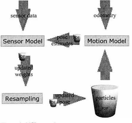
over allpossible poses.

A

high level diagram

ofthe

iterative

process

is

shown

in Figure 1

.

JMbg, _|

Motion Model

Resampling

.

*

^

T

[image:12.532.172.395.386.595.2]

2.1 Motion Model

Recall

the term p[x\x,_u a,_{

)

describes

the

probability

oftherobot's

position,

given previous position andtheactionundertaken.

To accurately

_portray thisa model must

be developed for

therobotthatcan

suitably describe

the

motions oftheplatformthatoccur as aresultof

any

willful action.

A

thoughtful

and correct application of

forward

kinematics

is

not

in

and of

itself

sufficientto represent_{this motion,}as real worldrobots are acted upon

by

allmannerof external

forces

thatcan

be impossible

tomodel. Robots are often subjectto

imperfections

in

theirownconstituent components aswell.

Consequently

an

important

part ofthismodel

is

theapproximationoferrors.

Typically

the

fastest

way

toarrive at such an estimation

is

to

study

therobot's perceived motion

in

a

variety

of environments.

Subsequent coaxing

ofthe

'error

picture'

allowsthe

model createdthrough

kinematics

to

be

revisedtogenerate position estimates.

The

robot used

for

testing

is

a

four

_wheeled, skidsteered rover whose macro

level

motions are composed of straight

line

translations and rotations aboutasingle point.

Data

was gathered

for both

typesofmovementand

is

alsopresented

in

the

following

sections.

2.2 Sensor Model

The

sensor model

facilitates

the

distillation

ofaccurateposition

information from

theavailable position

data,

and

is

represented

by

the p{o,\x,)

term

in

the

belief

equation.

Many

previousapplicationsof

MCL

leverage

sensors thatprovideenvironment

feature

data

and

distance information

implicitly

[4, 5, 6,

8]. This

simplifies

both

the

matching

problem andthe constructionofa

map

which

describes

theenvironmenttherobot will perceive.

However

thesesensors are

frequently

expensive_and, with

few

_exceptions,are

only

concernedwith

data

from

two

dimensions. Vision based

sensorsontheother

hand

yieldan

incredible

amount of raw

data

with which positional

information may be

derived,

though this richness of

information

comesatacost.

Adapting

MCL

for

use

in

vision

based

localization

presents several challengesthatmust

be

overcome.

A

significant

amount of_processingmust

be

performed on

data

yielded

by

thevision sensorto

derive both

a

map

and a sensor model.

Additionally

a suitable

frame

of reference

must

be

settledon,which

is

typically

tied

intimately

to thesensor model.

Vision

sensors arealsomore susceptibleto subtle changes

in

the

environment,

such as

lighting

and rotation or

scaling

ofthereferencewithrespectto therobot.

Further

attention

is

giventothese

issues in

sections

3

and

4.

The MCL

algorithm scales

nicely

asthecomputational

intensity

associated

is

a

direct function

ofthenumber ofparticles

being

maintained.

A

criticalmassof

3 Vision Based

MCL

For

all ofthereasons stated above

in

the

localization

survey,

MCL

is

thepreferred

technique

toarrive at a successful

localization implementation.

Particularly

benefits

relevantto thiseffort arethe

scalability,

neutral stance with respectto

sensing hardware

and generalrobustness

in

the

face

of errors.

MCL

has been

appliedwith monocular

vision as a

primary

sensor

in only

a

handful

of cases

[8,22,27].

The documented

applicationsthat exist

have

relied on a single

feature

matching

technique tocorrelate

vision

input

toa

database.

The final

goal ofthisresearchwill

be

to

implement

and maximizethe

efficiency

of

MCL

onthe

low

cost robotplatformthrough theuseof

multiple

computationally inexpensive

invariant features

_{and presentthe}

resulting

empirical evidence.

This

section

describes

the

initial development

of such a vision-based

MCL

implementation.

3.1

Research

Platform

Figure 2: Mauricetherobot

All

experimentation was conducted on

Maurice

therobot

(Figure

2),

a

custom platform

built specifically for

thisresearch.

Briefly,

Maurice is

a

skid-steered,

four

wheel

drive

rover with

built-in odometry

and

infrared

proximity

detectors

running

the

BusyBox

distribution

ofthe

Linux operating

system.

The

primary

sensor

is

a

CCD

camera withon-boardvideoprocessing.

Testing

and experimentation are

facilitated

by

CompactFlash

storage and

Ethernet

3.2

Motion

Estimation

The

motion modelthat

is

employed

is

relatively

simple.

The

shaft

encoders arethe

only

source of odometric

information

available onthe robot,

consequently

themodel

only

need

be

concerned withthese

inputs. Note

the custom robot platform

is

best

suitedto

navigating

about and

delivering

accurate

odometry

in

an environmentthatconsists of a single plane.

Consequently

the

Cartesian

coordinate system

has been

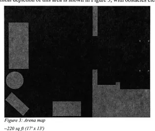
selectedtorepresent robotposition.

3.2.1 Environment

The

robot willoperate

in

an arena

roughly 220

square

feet in

area.

A

[image:15.532.100.417.209.478.2]

graphical

depiction

ofthis area

is

shown

in Figure

3,

withobstacles

clearly

visible.

Figure 3: Arena map

~220sqft(17'xl3')

3.2.2 Rotation Error

Modeling

Throughobservationsoftherobot motions

in

general,

it

was clearthat a

substantial

difference

exists

between

observed motion andthat

indicated

by

theon

board

odometry.

Witnessed

error

in

theplatform's motions are attributable to the

cumulative effects

from

a

variety

of sources.

Some

likely

sources

include

wheel

slippage, off-axis motor encodersand noiseonquadrature

decoder

interrupt

lines.

The

rotationalerrorsobserved are presented

in Figure 4. Results

have

been

grouped

for left

and rightturns

in

thesame_plot,whichcorrespondto to the

Rotation 400

350

300

250 CA 0)

200 0)

a

150

100

50

0

?Msasured

|

Actual

hftiiiiiiiiiiiiiiiiiiniii

13 5 7 9 1113 15 17 19 2123 25 27 29 3133 35 37 39 41

Trial

Figure 4:Degreesrotated,as measured

by

therobot and actual

While

error

data

is

consistent

for both left

and right_rotations,

it is

clear thata significant error component

is in

generalpresent

in

rotational motion.

Further

analysis ofthe trial

data

is

shown

in Figure

5,

wheretheapparent

proportionality

ofthe errorvalueto theamount of rotational motion

is

confirmed.

Rotation,MeasuredvsActual 400

100 150 200

Actual(degrees)

300

Figure 5: Erroras afunction ofactual rotation

It

is

presumedthat theerror_constant,

C

yielded

by

_{this analysis,}

is

largely

attributabletowheel _slippage,anunavoidableproblem

in

skid steered vehicles.

The

slope ofthesample

data

yieldstheconstant value

1.3695,

and sotheactual

Rotation

300

250

200

150

100

50

raActual _|

Actual

*C|

|

I

J

I

ill

-jM

-.Ii:lf

Liiiiili

1 3 5 7 9 11 13 15 17 19 21 23 25 27 29 31 33 35 37 39 41

Trial

Figure 6: Application ofskid-steer correction constant

The strong

errors observed are

largely

eliminated after compensation

for

the

linear

bias,

however

a non-trivial errorcomponent remainsas

illustrated below

in Figure

7,

withtheoutliers

indicating

errors of almost

15.

Capturing

thisnoise

is

criticalto thegeneration of reasonable guesses

during

particle

filter

operation.

ResidualError

15.00

10.00

5.00

0.00

-5.00

-10.00

-15.00

Figure 7: Error_remainingafter_{incorporation of}skid-steer

constant

A histogram

ofthisresidual component reveals a

Gaussian distribution

(plotted in Figure

8)

withamean

very

closetozero and a standard

deviation

of

about

5.

ErrorDistribution

J2

E

4^_

6

5 4 3 2 -P ,0 1 Z ? ^ i

u=0.2681;a=4.916

Figure 8: Histogram ofresidualerror

The

rotationalposition

for

thisplatform

in

themotion model

is

consequently

computed as

9=e^1+6'-C+randN{0.26Sl,

4.916)

where#'

is

the perceived_rotation, randN(mean, _stdev)yields arandom number

from

thenormal

distribution

defined

by

its

arguments and

C is

therotational correctionconstant

determined

previously.

3.2.3 Translation Error

Modeling

Translations

are constrained

by

thewheeledplatformto those that take the robot

forward

or

back along its

currenttrajectory.

These

straight

line

movements

are

generally

morewell

behaved

than theirrotational counterparts as

is

evidenced

by

the

data

shown

below in Figure 9. This data has been

capture

for both

types of

flooring

found in

thearenawheretestswill

be

conducted.

For

conveniencethis

data has been

consolidated

into

a single plot.

The

left

cluster

illustrates

trials

DistanceTraveled

1 3 5 7 9 11 13 15 17 19 21 23 25 27 29 31 33 35 37

Trial Number

Figure 9: Straight linemotion errors

Errors based

on

flooring

typeare negligiblewithrespecttostraight

line

motion,

but

significant when

heading

is

taken

into

account

(shown in Figure 10).

These

results

led

to the

discovery

ofa

slightly lethargic

motor onthe

front left

wheelof_{the robot,}whose

influence

is greatly

exaggerated on carpet.

This

is

attributedto the

higher friction

constantwhichprevents

it

from skidding

to

keep

up

withthe otherthreemotors.

The

net effect

is

a significant negative

heading

error whenevertherobot

is

onthis surface.

HeadingError

If

1

T

II

M

i i\

1

) 21 23 25 27 29 31 33 35 37

a_HeadingError

1

1

-2

-4

-6 <n

S,

-8 o a

-10

-12

-14

-16

Trial Number

Notice

that theperformance ofthe

MCL

algorithmshouldnot suffer

due

tothisextra noise

in

position estimation.

The

algorithm

itself

thriveson

limited

amounts of noisethatallow

it

toexplore all poses

in

thesearch space,as

long

as samples can

be

generatedthatreflecttheobservednoise

distributions. For

simple

turns,

which are effected

by

themotors

turning

in

opposite

directions,

the

heading

error

is

much

less

pronounced and can

be

computed with

only

theencoder error

factored in.

The

actual motion model employed

is

in

some ways crude.

The

encoder

advances

for

a given movement

(forward,

_{reverse, right,}

left)

aretracked

for

each

motor.

At

thecompletion of a_{movement, the} error

is

then

integrated

into

each reading,

yielding

a guess asto theactualpositionofeach motor.

This is

a

scientific approach

(noting

that theencoder positions can

be

expectedtoexhibit

normally

distributed

error),

however estimating

the

heading

error

in

straight

motions

is

decidedly

not so.

Since

slight errors

in

theencoders

may

occurat

any

time

during

therobot's_movement,

vastly different

effects can

be

observed on

its

resulting

orientation.

It

would

be

a

difficult

andtime

consuming

endeavorto

generate guesses about orientation errors

based

on real-time

data.

Instead,

a

rotational error

distribution is experimentally determined

andappliedtoyield

heading

errors aftereach respective motion

is

completed.

While

theencoder readings are

fairly

accurate,

displacement

errorsarestill

present and soneedto

be

accounted

for

to

bring

themotion model

in

line

withthe

actualplatform

behavior. These

errors are modeledasgaussian

based

onthe

interpolation

of

data from

thevarious

trials,

shown

in Figure 1 1

below.

Encoder ErrorDstribution

2_

18

IK

14/ , * count

i6 0)

3

AO

"o

/

8 n

E S z

/ c

1 A

P

-, ₄ i,

+--~

5 -4 -2 ) 2 4 (

u=

-0.6978;a=0.6356

It

is

worthwhiletonote that theerror

sampling based

onthesemodels

is

only

successful

because

it

is

performed

many

times

(once for

each particle

in

the

density

representation).

Hence

it

approximatestheactual_probability

density

error

function.

3.2.4 Application

of

Motion Model

To

_reiterate,

implementation

oftheerror modelontherobotplatform

grants

improved

position estimation and ameanstogeneratesample robot

positions

for

use

in

theparticle

filter. This

coupled witha

fairly

naive

kinematics

application completesthemotion model.

A

sample run ofthemotion model alone

appliedto thegeneric position

tracking

task

is

shown

below in Figure 12. In

this

sampletherobottraversedatotal

distance

of9'

8". A

mass of

500

particles

is

usedtoestimate the

probability density. The

robot

begins in

theupper

left

corner

andmoves

incrementally

along

an

arbitrary

pathtoward the

bottom

right.

At

each

increment

theparticlepopulation

is

drawn.

*

'<

f. _{\ JVr'vft}'joi?**;***.* 'A

-. * < '

',,'*" v'~'

\

':

*""

Figure12: Motionmodelappliedtogeneric position

tracking

task

Actualrobot position shown as solid red circle

Clearly,

errors compound

rapidly

when

only

themotionmodel

is

applied.

This helps illustrate

the critical

importance

of

reining in

position estimates

by

[image:21.531.140.397.279.528.2]

3.3 Sensor Model

Localization

cannot

be

performed

meaningfully

withouta

frame

of

reference.

This frame

of

reference,

or

map,

takes

different

shapes

depending

on

theavailable

sensing

equipment and sensor modelemployed.

Since

the sensor

model employed

here is based

on various

features

extracted

from

color

images,

it

is

appropriateto

build

a single common

image

library

from

whence all

feature

information

can

later be

extracted.

While it is

possiblethateach

feature

will

have

a preference

for

_{the number,}

quality,

orientation orresolutionofthese source

images,

keeping

this

initial

population constant should

facilitate

amore consistent

performance comparison.

A

library

consisting

of

624

images

was constructed

by

positioning

therobot at 18"

intervals

(both

xand

y

displacements)

acrossthetest

arena,eight orientations each(45

increments). Features

are extracted

from

the vision sensor and correlatedtoa

feature database

generated

from

this

library.

This

operation yields match probabilitieswhich

drive

thesensor update computation

by

revising

theparticle weights

in

the

PDF

representation.

In

other vision

based implementations

[8,22,27]

occupancy

grids or similar

mapping

strategies are usedto trackphysical

location in

additiontothe

map

supplied

by

the

feature

reference.

This

is in

a sense_redundant, asthe

image

library

already

retains positional

information for

the environment,

presuming

coverage

is

uniform.

The

work

described

here is

concerned

only

withtheground

truthprovided

by

the

feature library.

3.3.1 Na'ive Correlation

with

Color Histograms

Color histograms

are a suitable metric

for

differentiating

pose estimates

due

totheirrotationalandtranslational

invariance.

They

are also

easy

togenerate

andtake

comparatively little

spacetostore.

Another

convenient

property

is

the

easewith whicha

human

observercan gaugethe

similarity

of a

histogram

pair

by

inspecting

aplot ofthe

bins.

Consequently

a sensor model

based

on color

histograms

can

be

simplerthanother methodsto

debug.

Much

like

themotionmodel, the sensormodel must

be built

to

accurately

reflect

how

theenvironment

in

whichtherobot

localizes is

perceived

by

the camera.

The

notionof

comparing

color

histograms

themselves

is in

of

itself

simple,

however

thepeculiarities again of_{the platform, the}environment and

how

the two

interact

must

be

well understoodtopermittheextraction of meaningful

valuesto

drive

theparticle update.

Noise

thatexists

in

the system must

be

modeledtomaximizethe

likelihood

that

histogram

match

quality

reflectsthe

probability

thata sample

image

corresponds toa given position

in

themap.

The

map

was

implemented

asapopulationof color

histograms

generated

from

the

base

image

set.

A variety

ofreadingsweretaken

from

thecamerawiththe

lens

coveredtoestablish a noise

floor. This

wasthen

incorporated into

thesensor

sample

images

usedtogeneratethenoise

floor

andthe

resulting histogram

are shown

below

in Figures 13

and

14,

respectively.

Noise Floor

Figure 13: Sample imageused

tocalculate noisebias

Pixelvalue

intensity

enhanced

toillustratevariation

80

70

60

50

40

30

20

10

0

R_(noise)

G_(noise)

B_(noise)

- --

-L

J;

1 3 5 7 9 11 13 15 17 19 21 23 25 27

Bin

Figure 14: Color histogramnoisefloor

To

maximizetherelevanceofthenaive

image

compare

for

these

trials,

it

is necessary

tounderstand

how

theenvironmentappears

in

thecolor

histogram

space,

particularly

as perceived

by

the

CMUCam. Figure 15

showsthemaximum counts

for

each

bin

thatoccur acrossthe entirecolor

histogram library.

Clearly

theenvironmenttherobot

is operating in induces low

pixelvalues muchmore

Max_byBin

140

120

100

80

60

40

20

0

R

|

G: : B;

1 3 5 7 9 11 13 15 17 19 21 23 25 27

Bin

Figure 15: Maximumvalues

by

bin,

acrossentireimage

library

Tailoring

the

histogram

comparison

in

themanner

described

above

limits

its

use genetically.

However

bypassing

this

step

would come atthe cost of

reduced

sensitivity

andmore

frequent

errors

in image

matching.

During

localization,

this wouldmanifest as a

tendency

to

lose

good matches

during

the

resampling

step.

A

simple

differencing

_{measure, the}

Li-metric

is

suggested

in

[30]

for

histogram

comparison.

A heuristic

adaptation of_{this measure, termed}

"naive

correlation"

is

performedto

drive

theupdate

step

oftheparticle

filter

as shown

here,

where

N

is

theparticle_count, s_{the sample,}rthereference

image,

nthenoise

floor

andmthe

bin's

relevancemeasure.

N bins

quality

=

YdYdmax{i\shil-rbM\-nb

,),0)/

mbi

;=i 6=1

That

is,

for

each

bin in

_{the sample,}producethe

difference between

the

corresponding bin

of_{the reference,}removethenoise

bias

andscale

by

perceived

relevance.

Match quality for

asample

image (Figure

16)

is

plotted againsttheentire

image

library

in Figure 17. Note

the

step

_{characteristic,}which

is

attributableto

the sizable

differences in

lighting

between

the tworooms

in

thearena.

Additionally,

apronounced

clustering

ofmatch qualities

is

evident

between

0.3

and

0.7. This illustrates

one ofthe

difficulties

in using

color

histograms

solely

to

filter

position estimates.

The

inability

to

disambiguate

different

positions

strongly

may

result

in

positional uncertainty.

Ideally

sensorreadings should correlate with

Nafre Correlation

0.8

0.7

0.6 0.5

0.4

Figure16: Sample image

1?Quality

M?5Z

V4

zPSrz&f

700

Figure 1 7: Naivecorrelation matchquality,binbased

differencing

Resultsshownforeach_{entry image}

library

Figure 1

8

showsthe

top

five

matches

for

theprovided sample

image. The

heuristic

application results

in

a

quality

that

is

directly

proportionalto theparticle weight assigned.

This

correlation proceeds

by

first

identifying

the

location

and orientation

in

the

map

thatmost

closely

matchesthe current pose_{estimate, then}

using

the

heuristic

togenerate a

difference

measure.

pi

!

'*

;.:....

1 1

Figure 18: Samplenaivecorrelation, bestmatches

Match quality of0.838

(#452),

0.836

(#180),

0.832

(#524),

0.827

(#547)

and0.824

(#493),

A

sample

image (Figure

19)

is

comparedwiththe

best

fit

entry based

on

position

(Figure

20)

from

the

image library.

Figure 21 Shows

_{the red,}green and

blue

channel

histograms

superimposed.

Finally

the

resulting difference

measure

is

presented

in

Figure 22.

Figure 19: Sampled image

78.94xl5.98y-89

Figure 20: Reference entry

80.0"x

8.0"y

-90;

Entry

#27

Histogram Comparison(R) Histogram Comparison_(G) HistogramComparison(B)

Reference mReference

Sample

Reference

: Sarrple m

Sample

ill. ,

!

|

mm

.

Iffl

LtlllLk S ia B L

iiL

Ill,

Figure21: Comparison ofsample and referenceimage

Difference Measure

0.8

~ IbR

B

0.6

0.5

0.3

0.2

0.1

n

J_

]*-

III.,

i

1 3 5 7 9 11 13 15 17 19 21 23 25 27

Bin

Note

oneundesirable effect ofthis

heuristic is

thatasizable amount of

color

information

in

therangethatshows

up strongly in

thenoise

floor

is

discarded (Figure

23).

Consequently

the

difference

measure

has

undue

bias

towards

images

which

differ

distinctly

in

these

bins.

Max-Floor

140

-

120-100

-80

60

40

20

0

-20

-40

--60

in

JU

1 3 5 7 9 11 13 15 17 19 21 23 25 27

Bin

Figure 23: Adjustedreferencehistogram

Datashownisacross entireimage

library

3.4

Resampling

A

critical aspect oftheparticle

filter is

the

resampling

step

thatoccurs

between

applications ofthesensor modeland motionmodel.

This step dictates

how

theparticle population evolves.

In

its

most

elementary

form,

resampling

can

be

performed

by

simply

thresholding

theparticles

by

theirweight.

Repopulation

canthenoccur

any

number of_ways,e.g.

copying

surviving

particlesor random samples

from

thesearch space.

The resampling

techniqueemployed

in

this

implementation

propagates particleswitha

probability

equaltotheirweight

using

aselect withreplacement

technique

described in [31]. This

allowstheparticle masstomore

thoroughly

explorethosepositionsthatare

deemed

to

have higher

likelihood

by

thesensor

model,and should

keep

theparticle mass closeto the

ideal PDF. One

notable

problem with

importance resampling is its propensity for

tunnel-vision.

Because

it focuses

on

high

weightparticles,a single

bad

reading

could

drive

particle

weights

low

enough

for

themto

be

sampled out ofthe

population,

thereby

blinding

theparticle

filter

to

potentially

correct poses.

This

is

particularly

pronounced

in

the

kidnapped

robot_problem, and

is discussed further

in

section

3.5

Localization

Architecture

The

hybrid

control

hierarchy

is

a

promising

mechanism

for creating

a

responsive,

yet

deliberate

system.

This

approach grants amaximal amountof

flexibility

to the

design,

without

precluding

robustoperation.

A

control

hierarchy

loosely

based

onthisparadigm

has been implemented

on

top

ofthecustom

hardware (consult

appendices

A

and

B).

Since

theplatform cannot

localize in

real-time

due

to the

processing

constraints,

it

is

difficult

to

implement localization

as a

behavior

separate

from

the

behavior(s)

thatare

actually enacting

motion.

In

thetimethat

it

takes the

implementation

toacquire an

image,

process andupdatetheposeestimates, the

robot

itself

could

be displaced

orrotated enoughtocreate a

discontinuity

between

the

odometry

readings andthe

image

thatgets examined.

As

such, the

localization behavior is

subordinatedto themotion_control,which prevents

any

movement while

localization

processing is

underway.

A

_small,

but necessary

concession.

Note

that this approachwould not

impact

theresponsivenessofthe

robot

if

theplatform could

localize in

real-time.

However

localization

updates

wouldstill

be

atthe

mercy

ofthemotion

API,

which

is

probably

not

desirable.

For

example a single

forward

motionthat traversed5'would

only drive

one

3.6 Trials

The

localization

implementation

with naive

image

correlationwas putto

theposition

tracking

taskoverthecourse ofvarioustrials

described in

the

following

sections.

The

term'trial'

is

usedto

denote

asequence ofexperiments,

where each experiment or'run'conducted variesone or more

key

localization

parameters.

3.6.1 Success Indicators

The

taskof

localization itself is

somewhatsubjective, particularlywhen probabilistic estimation methods are_employed,as

rarely if

ever will a robot

be

abletoposita guesswith

100

confidencethat

exactly

mirrors

its

real

location. For

trials conducted

here,

the

localization

effort

is deemed

successful

if both

ofthe

conditions

below

are met.

Greater

than

90%

_oftheparticles are centered about a single point

The

standard

deviation from

thecenter

of

mass

of

theseparticles

is less

than

10%

of

thearena

dimensions.

For

the testarenathesecond measureabove equatestoa circular region

1

foot in

diameter.

Essentially

it is

requiredthataperceivedcollapseofthe

PDF

occurs about a single pointwithan

arbitrary

threshold.

A localization

run

is deemed

a

failure if

eitherofthe

following

conditions are met.

The

time taken to

localize is

inexcess

of 5

minutes

3.6.2 Position

Tracking

Being

ableto

consistently

present an estimate of robotposition

is

acritical

component of a

localization

strategy.

The

first

trial

is

consequently concerned

with

determining

thesuccess ofthe

localizer

with respectto theposition

tracking

task,

which

differs from

global

localization (presented

in

the

following

section)

only

by

the

initial

position estimatethat

is

suppliedtothe

localizer. That

is,

the

particle population attimezero

has

zerovariance and

is

centered aboutasingle

coordinate.

The

taskputto therobot requiredthe traversalof a

distance

of

1000"

(-83')

while

remaining

well

localized.

Results

for

a

largely

successful position

tracking

run are shown

below. The

paththerobot

actually followed for

thisrun

is

illustrated in

Figure 24.

FP? arugfr

C!KUfcCifri.i-F:.aj;;':

COTMWlVlfW :lW#*WMsn JHI*JIOT _\OW$ CoKf Mt*Wl

'

Sttf* ;SfTW

[image:30.532.112.420.242.520.2]

> ! hWK ;WTK !~ i*I C*tof4 fiiirit*NW

Figure 24: Position_trackingtrialpath

Distancetraveled-₆₁

feet;

_{Arrow indicates startingposition;}

The final

particle population

is

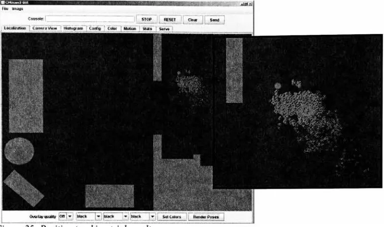
shown

in Figure 25. Position

estimates are

clustered

in

a

16"

radius aroundthe actual robot

location. Note

that theactual

density

can

be

difficult

to

interpret based

onthisgraphicalrepresentation,as

high

Figure 25: Position

tracking

trialresult

Localizer'sfinalposition estimate shown ashollowcircle;Actualpositionshown as solidcircle; Finalposition confidence

0.97;

Finalerror

10";

5000particles

A

range of

data

collected

from

thistrial

is

plotted

in Figures 26

and

27.

Data

is

shown

for

particlecounts1

vs.the

distance

traveled towardsthe 1000"

goal.

Runs

that

did

notachievethegoal are givencredit

for

the

distance

traversed

priorto

leaving

the'well-localized' state.

Goal

? Traveled

Log.(Traveled)

- - Goal

DistancevsLogParticles Distancevs.Particle Count

Particles(10Ax)

Figure 26: Distancetraveledvs particle count, logarithmicscale

1400

1200

1000

800

600

400

200

0

?^-^

:tl

[image:31.532.74.464.61.292.2]

0 20000 40000 60000

Figure 27: Distancetraveledvs particle count

Surprisingly,

therobot was ableto track

its

position

relatively

wellat

very

low

particle

counts,

despite

never

meeting

thegoal.

In

one

instance it

managedto

travel573.13"while

operating

the

localizer

on

only 100

particles.

While

periodically

the

localizer

developed

multiple

hypothesis

aboutthe

current robot

position,

the

only

conditionthatpreceded a

failed

trial

(in

all

cases)

was a

lack

of pose estimates at or

very

closeto therobot's actual position.

This

dearth

of

samples,

or sample

impoverishment,

is

solely

a

function

ofthenumber of

particles availableto theparticle

filter.

In

practice

it

is

one ofthe

few

occasions

wherethemass of particles

does

an

inferior job

of

representing

thecontinuous

PDF.

As

thenumber of particles employed approaches

infinity

theparticle mass

becomes indistinguishable from

the

PDF.

However,

for

realisticparticle numbers

it is

usefultounderstandwhatthe

'critical

mass'

is. That

is,

atwhat point

does

the

implementation

sufficiently

estimatethe

PDF? Based

ontheexperimentation

conducted

in

thisand othertrials

described

below,

thatnumber

is

consistently

at

or

just

above

2,000. It

is important

tonote that

impoverishment

was witnessed at

and above_{this number,}

however it

was always caused

by

uneventerrain

in

the

arenathat

induced

severe rotational errors.

In

thiscasethemotion modelwas not

abletogenerate samples consistent with actualrobot motion.

This

is indicative

of

thesorts of problems real world robots encounter.

An

appropriate responseto thesample

impoverishment

scenario might

be

torelaxthemotion_model,andevento attempttoaccount

for

extreme errors

due

tounforeseen

interactions

withthe environment.

However modeling

unobservable errors would

be

a

decidedly

unscientific_endeavor,

further,

the

likelihood

of

generating

anappropriate samplewhen_say, therobot

falls down

a

flight

of_stairs,

is

small.

Another

approachmight

be

topermit

resampling

to some

extent,

from

a uniform

distribution

overthesearchspacewhenevermatch

quality

dips

below

a

dynamic

threshold.

High

particle countswould

be

requiredtoensure

anappropriate numberof samples are generated outside ofthe central particle

mass.

Alternatively,

theuse ofthe

dual

of

MCL

[7]

may be

_warranted,where

replacementoccurswithsamples

drawn from

a pool of pose estimatesthatare

consistentwith sensorreadings.

Contrast

this

latter

approachwith

MCL

as

previously

discussed,

wherepose estimates are generated

only

through

odometry

andvetted

by

sensor

inputs. To

_{generalize, the}sample

impoverishment

problem

described

here is

really

just

a

less

extreme caseofthe

kidnapped

robot_problem,

In

additionto

continuously supplying

a poseestimate,

it

is

important

to

quantify

the

accuracy

oftheseestimates

in

determining

theoverall effectivenessof

the

localization

implementation.

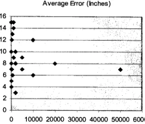
Average

error recordedoverthe courseofthe

trial

is

presented

in Figure 28

for

each_run,with averageerror per unit

distance

traveledshown

in

Figure

29.

Runs

are ordered

by

particlecounts,

from lowest

to

highest.

Average Error_(Inches) Errorper unitdistance

?

? ?

? ? ?

? ?

Error/distance Log.(Error/distance)

[image:33.531.78.221.157.280.2]

10000 20000 30000 40000 50000 60000

Figure 28: Averageerror vs particles Figure 29: Errorper unit

distance;

At first

glance

it

appearsthatpositional

accuracy increases

withthe

number of particles.

However

the trend

in Figure 29 falls

off

largely

due

to

low

particle count runs not

meeting

_{the goal,}and

consequently

traversea smaller

distance. Figure 30

showstheproportional error whenthe effect of

distance is

eliminated.

Proportional Error

[image:33.531.256.421.158.282.2]

1 3 5 7 9 11 13 15 17 19 21 23 25 27

Figure 30: Proportionalerror

Shownwithrespecttothe

1000" goal

For

theposition

tracking

task,

theaverage error

is

consistent and appears

to

be independent

of particle count at aratio of about0.009/1000"

(9"). Errors

were

occasionally

witnessed

in

excess of

30",

but

typically

therobot's position

estimate

hovered between

0"

and

16"

[image:33.531.169.327.400.526.2]

To summarize,

theparticle count appearsto

only

affectthe

likelihood

that theparticle

filter

won't exhaust

its supply

of position estimates.

Beyond

this,

somewhat

counterintuitively,

_positional

accuracy

appears

independent

ofthe particle population size.

To

improve

upontheseresults

it is important

to

understand what

exactly is motivating

thewitnessed errors.

At first

glancetherearetwo typesof

localization

errorsto

be

concerned

with

beyond

those

previously

discussed,

positional

inaccuracy

and positional

uncertainty

(Figures

3 1

and

32,

respectively).

The

former

refersto

distance

between

estimated and actual robot_position,whilethe

latter

tostandard

deviation

(which is essentially

the

inverse

oftherobot's confidenceabout

its

position

estimate).

Clearly

both

ofthese terms

impact

theusefulnessofthe

localization

results.

Figure 31: Position

inaccuracy

_{Figure 32: Positional uncertainty}

It

is

hard

to assign

blame

to

any

specific

step

undertaken

during

the

localization

_process, astheposition estimate

is

a product oftheirclose

interaction.

It

is

possiblethat themotion model

is

failing

to generate appropriate samples.

However,

early

position

tracking

trials

employing only

the motion model

(Figure

12)

wereverified

repeatedly

toproducecorrect particle

densities according

to robotmotion.

The

successeswitnessed

in

the

first

trialwithrespectto

longer

distances

traveledwould alsoseemtorule out sucha conclusion.

It

is

possiblethat

the

resampling

algorithmemployed

is

doing

an

unsatisfactory job

of

removing

poorestimates

from

thepopulation.

Were

this the case

it

should

be

possibleto

reduce

both

errorterms

by

adding

more sensor

data

without

introducing

new

samplepositions.

In

practicethiscan

be

accomplished

by

rotating

therobot about

its

axis repeatedly.

Figure

33

showstheprogressionof a

reasonably

well

localized

Deviation fromposition estimate

1 4 7 10 13 16 19 22 25 28 31 34 37 40 43

Step

Figure 33: Effect ofadditional measurements ondeviation

The

behavior

visible

in

thecurve shows thatadditional sensor

information

motivates an

improvement

in

overall confidence.

However

therepeated

culling

of

theparticle population withouttheadditionof motion modelsamples

is

probably

driving

the estimatetowards the

best

matches

in

the

image

library

artificially.

This

approachunderminestheprobabilistic nature oftheparticle

filter. Moreover

it

is

unlikely

toallowthe

localizer

toarrive attheactual robot positionestimate

due particularly

to

differences between

reference positionsand_samples,

but

also

because

of

lighting

variations,

image

noise andunexpectedobstructions.

Permitting

resampling

tooccur as

solely

a

function

oftheparticle

probability

allowsthe

localization implementation

to

stay

true to

its

mathematical

foundation.

Closer

inspection

ofthesensor model's

behavior

overthecourse ofa

few

trialsreveals acentral

issue

thatwas alludedto

in

section

3.3. Figure 34 depicts

a

particlepopulation superimposedover a representation of samplematch

quality

with respecttothereferencemap.

A group

of

8

circles

is

positioned about a

single reference

location,

each

corresponding

toa reference orientation.

Circle

diameter is

proportionalto thereported

quality

ofthematch performed onthe

c_{OO Oo}0 000

O 0 0 0 0

1

>o0 O_OB;v 000

k'A~-'

OO * *

fgOOP*

%

000 o *w&\

., O -''**

^

0*& 0 O

o_Q o OO .. <ito OO oOO

'

0ci'

i ft)

#

e* *

o

600

, 000 OOO

O O 0 g. ? 0

<_{O '.}.

oo( *

4>P #'s

, <ooo

,%v* t *v

*,

*

<*

? 0 0O O * 000 OOO

0 0 * _{0 0 0}

[image:36.532.172.366.58.253.2]

. 0 ?_{00 000 OOO}

Figure 34: Imprecisionduetosensor model_ambiguity

200particles,globallocalizationtrial

Match qualityforthecurrent sample shownfor 8orientations at each reference positioningreen. Circlediameterisproportionaltomatch

probability

At

_{this position, the} sensor modelwill

likely

be

unableto

further

refinethe

positionestimate

due

to the

ambiguity in

the

image

correlation.

While

the

probabilities arenot_equal,

they

are close enoughto

delay

the

ideal

collapseofthe

PDF

almost

indefinitely. The ambiguity

evident

here is

atthecoreofthe

3.6.3

Global Localization

To

measuretheeffectiveness againsttheglobal

localization

problem, the

robot was movedtoa random

location

in

theroom and setaboutthe

localization

task.

A

sample run

from

this trial

is

presented

below,

withthepaththerobot

followed

shown

in Figure

35.

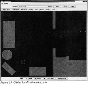
[image:37.532.98.407.142.437.2]

; CjrvxwnWw l.rcifl*wi W?trf|T.,m :Ovflg Crtw ; Jrt>n 51*3 iSww twaatz_|CamgraRwa.f irB" if'

Figure 35: Global localizationtrialpath

This

particular run resulted

in

a

localization

failure,

theprogression

is

shown

in

Figure 36. Significant

errors were witnessed whenturnswere executedon a transition

from

woodtocarpeted

floors. The

errors measuredwereoutside of

threestandard

deviations

oftheexpectederror

built

into

themotionmodel

for

rotationalmotions.

This

coupledwith sample

impoverishment

putthe

localizer

in

an unrecoverable state.

Leaving

therobot

doomed

towanderthe arena withan

incorrect

position estimate until

surviving

samples

by

chance

overlap

withthe

[image:38.532.52.482.58.288.2]

Figure 36:Sampleimpoverishmentandoverlyoptimistic motion model

Failedgloballocalizationtrial, 500particles; Conferwith pathinfigure35

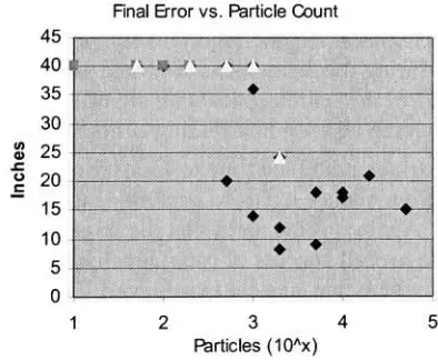
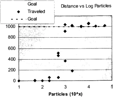
The

final

error value results

for

the trialwhichthisexample

is drawn from

are shown

in Figure 37. Clusters

of runswherethis situation arose are marked

by

square points

in

theplot.

Triangular

points markruns wher