Ray-based segmentation algorithm for medical imaging

This is a repository copy of

Ray-based segmentation algorithm for medical imaging

.

White Rose Research Online URL for this paper:

http://eprints.whiterose.ac.uk/148735/

Version: Published Version

Proceedings Paper:

Danilov, VV, Skirnevskiy, IP, Manakov, RA et al. (3 more authors) (2019) Ray-based

segmentation algorithm for medical imaging. In: International Archives of the

Photogrammetry, Remote Sensing and Spatial Information Sciences - ISPRS Archives.

International Workshop on “Photogrammetric & Computer Vision Techniques for Video

Surveillance, Biometrics and Biomedicine", 13-15 May 2019, Moscow, Russia. , pp. 37-45.

https://doi.org/10.5194/isprs-archives-XLII-2-W12-37-2019

[email protected]

https://eprints.whiterose.ac.uk/

Reuse

This article is distributed under the terms of the Creative Commons Attribution (CC BY) licence. This licence

allows you to distribute, remix, tweak, and build upon the work, even commercially, as long as you credit the

authors for the original work. More information and the full terms of the licence here:

https://creativecommons.org/licenses/

Takedown

If you consider content in White Rose Research Online to be in breach of UK law, please notify us by

RAY-BASED SEGMENTATION ALGORITHM FOR MEDICAL IMAGING

V.V. Danilov1, 2, _{*, I.P. Skirnevskiy}1_{, R.A. Manakov}1_{, D.Yu. Kolpashchikov}1_{, O.M. Gerget}1_{, A.F. Frangi}2

1 _{Medical Devices Design Laboratory, Tomsk Polytechnic University, 634050, Tomsk, Russia} – _{[email protected],}

(skirnevskiy, ram8, dyk1, gerget)@tpu.ru

2 _{Center for Computational Imaging and Simulation Technologies in Biomedicine, University of Leeds, LS2 9JT, Leeds, United}

Kingdom – (V.Danilov, A.Frangi)@leeds.ac.uk

Commission II, WG II/5

KEY WORDS: Segmentation, Medical Imaging, AdaBoost.M2, RUSBoost, UnderBagging, SMOTEBagging, SMOTEBoost

ABSTRACT:

In this study, we present a segmentation algorithm based on ray casting and border point detection. The algorithm’s main parameter is the number of emitted rays, which defines the resolution of the object’s boundary. The value of this parameter depends on the shape of the target region. For instance, 8 rays are enough to segment the left ventricle with the average Dice similarity coefficient approximately equal to 85%. Having gathered the data of rays, the training datasets had a relatively high level of class imbalance (up to 90%). To cope with this issue,ensemble-based classifiers used to manage imbalanced datasets such as AdaBoost.M2, RUSBoost, UnderBagging, SMOTEBagging, SMOTEBoost were used for border detection. For estimation of the accuracy and processing time, the proposed algorithm used a cardiac MRI dataset of the University of York and brain tumour dataset of Southern Medical University. The highest Dice similarity coefficients for the heart and brain tumour segmentation, equal to 86.5±6.9% and 89.5±6.7%, respectively, were achieved by the proposed algorithm. The segmentation time of a cardiac frame equals 4.1±2.3 ms and 20.2±23.6 ms for 8 and 64 rays, respectively. Brain tumour segmentation took 5.1±1.1 ms and 16.0±3.0 ms for 8 and 64 rays respectively. By testing the different medical imaging cases, the proposed algorithm is not time-consuming and highly accurate for convex and closed objects. The scalability of the algorithm allows implementing different border detection techniques working in parallel.

1. INTRODUCTION

Image segmentation entails dividing up a digital image into one or more meaningful regions. Active research on this problem has been conducted for over four decades (Cremers et al., 2007). This fundamental problem in computer vision can be solved by a variety of algorithms. Each algorithm has its own advantages and disadvantages. Some of the widely used algorithms were considered in (Danilov et al., 2018, 2017; Noble and Boukerroui, 2006; Pham et al., 2000). In several contexts, there is often a need to obtain segmented images. In medicine, there is an interest in obtaining digital 3D models of organs. The latter is linked with analysis and surgery planning (Dey et al., 2009; Lynch et al., 2008). Some segmentation algorithms depend only on image intensities, for instance, thresholding (Lee et al., 1990; Sankur, 2004) or k-means clustering algorithms (Ng et al., 2006). Other methods use spatial information, such as region growing, deformable models, and watershed segmentation. Finally, some approaches to image segmentation algorithms use statistical parameters, the first/second raw/central moments (mean and variance), and experimental distributions combined with statistical distances such as the Bhattacharyya distance, the Mahalanobis distance, total variation distance, Kullback–Leibler divergence and Jensen–Shannon divergence (Hu et al., 2010; Katatbeh et al., 2015; Li et al., 2013; Reyes-Aldasoro and Bhalerao, 2006). Some papers consider the global histograms, shape gradients and information theory to segment the region of interest (Herbulot et al., 2006; Junmo Kim et al., 2005). This class of segmentation techniques involves shape gradient and mathematical computations for the level set equations. This class of approaches leads to non-convex methods. The latter means they are sensitive to the initialization choice and only compute a local minimizer of the energy.

* Corresponding author

Graph-based algorithms represent other class of segmentation (Ayed et al., 2010; Gorelick et al., 2012). These algorithms are used for computing the accurate global minima without level set representation. One of the main disadvantages of these algorithms is the restriction by different distances such as 2

distance, Bhattacharyya distance or L2 norm.

Several segmentation methods are based on machine learning (Gorelick et al., 2012; Noble and Boukerroui, 2006). Such methods have several restrictions, and one of them is manually labeled data. The amount of this data should be relatively big and heterogeneous, to train a classifier/network with a high level of accuracy and absence of overfitting.

The image segmentation techniques can be applied to both three-dimension and two-three-dimension domains. Recently, 3D modalities have become popular in medicine. A large number of non-invasive cardiac and other diagnoses are performed by MRI (magnetic resonance imaging) and CT (computed tomography) (Katatbeh et al., 2015). The output data of these modalities has a three-dimensional format. However, two-dimensional image processing is still relevant. In some cases, 3D segmentation problems can be dealt with efficiently as multiple 2D problems (so-called 2.5D analysis) as, for instance, in the cardiac chamber or brain tumour segmentation.

In this paper, we describe a 2D automatic segmentation algorithm based on the spatial generation of rays used as detectors of the border point for the target region. The proposed algorithm requires minimal user interaction since it has only one global parameter – several emitted rays. The algorithm can be easily implemented in the image processing systems, including medical imaging systems, due to its efficiency, simplicity and execution speed. The latter allows using the algorithm in real-time for two-The International Archives of the Photogrammetry, Remote Sensing and Spatial Information Sciences, Volume XLII-2/W12, 2019

dimensional imaging. If the region of interest has a circular shape with an eccentricity value close to zero, then the small number of rays are required to perform segmentation for a relatively short time. Another advantage of the algorithm is its low sensitivity to noise due to the analysis of the ray data, rather than the whole image. The algorithm is practically insensitive to contour breaks, which is a crucial feature of segmentation algorithms.

2. SYSTEMS AND DATA

As a source of data for the heart chambers segmentation, we used short-axis cardiac MR images, which were acquired for 33 patients with different diagnoses (Andreopoulos and Tsotsos, 2008) by courtesy of York University (York, United Kingdom). Each patient’s dataset consists of 20 frames and 8-15 slices along the long axis. The size of each frame is 256*256 pixels. To test the proposed segmentation algorithm, we chose 3 subjects with different diagnosis (a 17-year-old patient with no cardiac disorders, a 16-year-old patient with Marfan syndrome, and a 9-year-old patient with severe aortic insufficiency). The dataset images were manually segmented where both the endocardium and epicardium of the left ventricle (LV) were visible. The ground truth of left ventricles' endocardial and epicardial was performed by two clinicians (Radiologist-in-Chief and Cardiac Radiologist).

As a source of data for the brain tumour segmentation, we used brain tumour dataset T1-weighted contrast-enhanced images from 233 patients with three kinds of brain tumour: meningioma, glioma, and pituitary tumour (Cheng et al., 2016, 2015). This dataset was acquired at Southern Medical University (Guangzhou, China). The size of each frame is 512*512 pixels.

Patient records and information were anonymized and de-identified prior to analysis. The brain tumour dataset was approved by the Ethics Committees of Nanfang Hospital and Tianjin Medical University. The cardiac dataset provided by the Department of Diagnostic Imaging of the Hospital for Sick Children in Toronto and the University of York. It is publicly available and provided for research purposes only.

The data were pre-processed on a computer, equipped with an Intel Core i7-4790K CPU (4.0 GHz) and NVIDIA GeForce 960 GT graphics card, using MATLAB 2018a on Windows 10. All classifiers were trained on a C5 instance (C5 High-CPU Quadruple Extra Large) of Amazon Web Services using R 3.5 on Linux Ubuntu 16.04.

3. METHODS

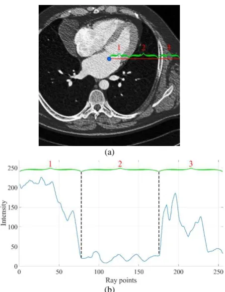
The main idea behind the proposed approach is to distinguish two classes based on a ray profile. The ray profile represents a one-dimensional array. Using one-one-dimensional input data (rather than two-dimensional or three-dimensional input arrays) allows decreasing the complexity of the classifier. An intensity profile of a ray is shown in Figure 1.

(a)

(b)

Figure 1. Data acquisition along the ray: an emitted ray (a) and its intensity profile (b)

The common workflow of the proposed algorithm is reflected below in Table 1.

Step Training Inference

1 Pre-processing and

normalization

Pre-processing and normalization

2 Truncated ray emission Full ray emission

3 Data gathering Data gathering

4 Classifier training Classifier inference

5 – Post-processing

Table 1. Algorithm workflow for training and inference

3.1 Pre-processing

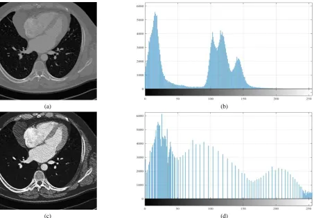
For the proposed approach there are no limitations for application of pre-processing techniques. No pre-processing can also be applied. In our case, we used a bimodal Gaussian function as a general filtering method since it depends on the histogram of the input image. This method of adaptive equalization presented by Pizer et al. (Pizer et al., 1987) is considered universal. After implementation of this step, the dynamic range of the image was expanded, which allows displaying previously unseen details (Figure 2). And a cardiac MR image of this section is only used for the explanation of the main concept of the proposed algorithm.

3.2 Ray emission

The next step involves the generation of ray sets and gathering the data along the rays. To get training and testing datasets, we gather five ray sets for each image. This number is data-specific and depends on a certain case. Coordinates of starting points for each ray set are assigned randomly within an image. We have experimentally found out that the closer initial point is to the centroid of the region, the higher border detection accuracy is obtained. For instance, MATLAB regionprops function can The International Archives of the Photogrammetry, Remote Sensing and Spatial Information Sciences, Volume XLII-2/W12, 2019

return a centroid (centre of mass of the region) and/or a weighted centroid (centre of the region based on location and intensity value). As for ray generation, we used the polar coordinate system with the origin at the starting point. The rays were propagated in all directions with a different change of angular

steps ∆ . The optimal angle change, which is equal to /16, was chosen experimentally since it maintains a balance between the processing time of the algorithm and the output segmentation accuracy. Ray emission is shown in Figure 3. The angular step in this figure equals to /4 and is only used for simplicity.

(a) (b)

Figure 3. Visual representation of ray emission: pre-processed source image (a) and manually labeled mask (b)

There is a difference between gathering the ray data during training and inference steps. The data for the training step is acquired within the area restricted by a mask (blue rays of Figure 3) going a little beyond the borders. The inference step assumes collecting the data along the entire length of the rays (red rays of Figure 3).

Once the rays are obtained, we can apply any binary classifier to border detection. However, the length of each ray varies. The latter imposes a restriction on the classifier since almost every machine learning technique requires fixed-length input data. To manage this problem, we divide each ray into fixed-length one-dimensional patches. We used different kernels and strides for the rays to figure out which set of parameters is best to apply. The generation of the fixed-length patch-based dataset is reflected in Figure 4. The upper row represents a ray mask, while the lower row is the grayscale normalized ray data. The values in blue boxes refer to the labels, representing border existence (stepwise increase/decrease). For simplicity, we used kernel size equal to 3 in Figure 4. However, for the experiments, we used kernels sizes of 5, 7, 9, and 11. As for stride, its value varies from 1 to 7 namely 1, 3, 5 and 7. The higher the kernel and stride values are, the fewer samples the dataset has. For instance, a dataset with kernel = 5 and stride = 1 has 955,726 samples. A dataset with kernel = 11 and stride = 7 has 151,251 samples. It worth noticing that lower values of kernel and stride tend to stronger dataset imbalance. The dataset with kernel = 5 and stride = 1 has 87:13 class ratio, while the dataset with kernel = 11 and stride = 7 has 70:30 class ratio.

Figure 4. Example of gathering fixed-length one-dimensional patches with their labels.

(a) (b)

(c) (d)

Figure 2. Image enhancement using the bimodal Gaussian function: source image (a) and its histogram (b), enhanced image (c) and its histogram (d)

The International Archives of the Photogrammetry, Remote Sensing and Spatial Information Sciences, Volume XLII-2/W12, 2019

3.3 Classifiers

As described before the acquired datasets are class imbalanced. In some cases, the negative class is 8 times more frequent than a positive one. The classifier’s goal is to identify the minority class i.e. the border. One of the efficient ways to manage imbalanced datasets is to balance them either by oversampling instances of the minority class or under-sampling instances of the majority class. However, such simple sampling approaches have drawbacks. Oversampling the minority class can lead to model overfitting, since it will introduce duplicate instances, drawing from a pool of instances already small. Similarly, under-sampling the majority class can leave out important instances that provide important differences between the two classes. However, there exist more powerful sampling methods that go beyond usual oversampling or under-sampling techniques. The most well-known example of such methods is Synthetic Minority Over-sampling Technique (SMOTE), which actually creates new instances of the minority class by forming convex combinations of neighboring instances (Chawla et al., 2010; Galar et al., 2012). As Figure 5 below shows, it efficiently draws lines between minority points in the feature space and samples along these lines. This allows balancing a dataset without as much overfitting, as it creates new synthetic examples rather than using duplicates. Nevertheless, this method does not prevent all overfitting, as these are still created from existing data points.

Figure 5. Visualization of SMOTE technique

Another popular sampling technique is the Random Undersampling algorithm (RUS). It creates a new dataset comprising of all instances from the minority class and a random selection of instances from the majority class.

To manage the problem of border classification based on imbalanced datasets, we chose the following ensemble-based classifiers:

1. AdaBoost.M2. This is an extension of AdaBoost, introducing pseudo-loss, which is a more sophisticated method to estimate error and update instance weight in each iteration compared to regular AdaBoost and AdaBoost.M1 (Galar et al., 2012).

2. RUSBoost. This method is based on AdaBoost.M2 and

it uses random under-sampling to reduce majority instances in each iteration of training weak learners. A 1:1 under-sampling ratio (i.e. equal numbers of the majority and minority instances) is used (Galar et al., 2012; Seiffert et al., 2010).

3. UnderBagging. This method uses random

under-sampling to reduce majority instances in each bag of bagging in order to rebalance class distribution. A 1:1 under-sampling ratio (i.e. equal numbers of the

majority and minority instances) is used (Galar et al., 2012; Lu et al., 2016).

4. SMOTEBagging. This method uses both SMOTE and

Random Over-Sampling (ROS) to increase minority instances in each bag of bagging in order to rebalance class distribution. The manipulated training sets contain equal numbers of the majority and minority instances, but the proportions of minority instances from SMOTE and ROS vary for different bags, determined by an assigned re-sampling rate (Galar et al., 2012; Wang and Yao, 2009).

5. SMOTEBoost. This method is based on AdaBoost.M2

and it uses SMOTE to increase minority instances in each iteration of training weak learners (Chawla et al., 2010; Galar et al., 2012).

All aforementioned methods are originally implemented with decision trees; however, we used other supervised learning algorithms to build weak learners within ensemble models. The learning algorithms used to train weak learners within the ensemble models are Classification and Regression Tree (CART), C5.0 Decision Tree (C50), Random Forest (RF), and Naive Bayes (NB). If the classifier finds no border point within a ray, then this ray will be ignored.

3.4 Metrics

The problem of classification deals with the trade-off between recall (percent of positive instances classified as such) and precision (percent of positive classifications truly positive). However, when instances of a minority class are detected, we are usually concerned more so with recall than precision, as in detection, it is usually more costly to miss a positive instance than to falsely label a negative instance. When comparing approaches to imbalanced classification problems, it is better to consider using metrics beyond binary accuracy such as recall and precision. Such metrics as accuracy and specificity become inefficient since they achieve high values because of the strong predominance of the minority class. In addition, we estimated the harmonic mean of precision and recall – F1 score. It should be additionally noted that it is preferable to assess the ROC curve when there is a need to give equal weight to both classes’ prediction ability.

3.5 Post-processing

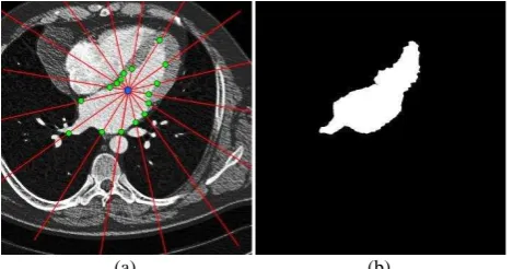
Once the border points are detected, the algorithm connects them smoothly. To perform this step more accurately, the periodic interpolating cubic spline curve is applied (Lee, 1989). A mask is obtained based on a received contour. An example of 16-ray segmentation is shown below in Figure 6.

(a) (b)

Figure 6. Set of border points obtained by the classifier (a) and a mask obtained after post-processing step (b)

The International Archives of the Photogrammetry, Remote Sensing and Spatial Information Sciences, Volume XLII-2/W12, 2019

4. RESULTS

In this section, we describe the results obtained both for border detection and following segmentation task. As described before, recall, precision, and F1-score are used to estimate border detection accuracy. Additionally, we studied how the accuracy and processing time change regarding the different values of ∆ and a different number of emitted rays. The Dice similarity coefficient (DSC) was the main metric for segmentation accuracy estimation. We have also analyzed the dependence of segmentation results on the shape of a region.

4.1 Border detection

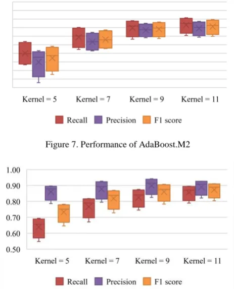
To estimate border detection performance, 5 classifies were used (AdaBoost.M2, RUSBoost, UnderBagging, SMOTEBagging, and SMOTEBoost). Each classifier has been trained on 16 datasets, where each dataset varied between four kernels (5, 7, 9, and 11) and four strides (1, 3, 5, and 7). However, stride change did not influence the performance while kernel change affected the border detection accuracy. Performance is visualized for different kernel values and stride equal to 1. Classifiers trained on stride of 1 have the highest performance in comparison with the ones using a stride of 3, 5, and 7. Performance of the studied classifiers is reflected in Figure 7–11.

Figure 7. Performance of AdaBoost.M2

Figure 8. Performance of RUSBoost

Figure 9. Performance of UnderBagging

Figure 10. Performance of SMOTEBagging

Figure 11. Performance of SMOTEBoost

All classifiers with kernel size equal to 11 showed a relatively high level of performance. While 5 features are not enough for classifiers to have a good quality of prediction. It should be also noted that RUSBoost, UnderBagging, and SMOTEBagging have a high value of precision and relatively low level of recall with kernel equal to 5. These classifiers manage well with the majority class (background pixels) and badly with minority class (border pixels). AdaBoost.M2 with pseudo-loss and SMOTEBoost perform classification task better and more reliably.

As an additional performance metric, training time was estimated. Estimated training time for the classifiers is shown in Table 2. Only reduced versions of datasets containing 50,000 samples were used for testing. The machine for algorithm time testing was based on C5 instance of Amazon Web Services and is described in more detail in section 2.

The International Archives of the Photogrammetry, Remote Sensing and Spatial Information Sciences, Volume XLII-2/W12, 2019

CART C50 RF NB

AdaBoost.M2 30±9 85±21 80±15 211±42

RUSBoost 13±7 54±19 35±14 211±46

UnderBagging 8±4 23±11 29±15 42±9

SMOTEBagging 57±20 104±30 144±31 70±23

SMOTEBoost 568±452 647±471 610±431 709±440

Table 2. Training time for the classifiers in seconds (mean ± standard deviation)

As seen, the most time-consuming classifier is SMOTEBoost. It should be additionally noted that the Naive Bayes learning algorithm increases the training time for all classifiers. The least time-consuming combination is UnderBagging based on the Classification and Regression Tree learning algorithm. The most accurate combination, AdaBoost.M2 based on Random Forest, took an intermediate position in the training time ranking.

4.2 Heart segmentation

As described in Section 2, the data acquired at the University of York was used to test the proposed algorithm. The examples of the left ventricle segmentation are presented below in Figure 12.

Figure 12. Segmentation of the LV performed by the proposed algorithm (blue) and manual delineation (red)

To test the accuracy and processing time of the heart segmentation, we used a dataset, which included 156 slices. Segmentation accuracy for different parameters is shown in Table 3. In our case, the target anatomical structure (left ventricle) for heart segmentation has a circular shape with an eccentricity value close to 0. It means that in such a case, a few

rays (large value of angle change ∆ ) are enough for obtaining the relatively high value of accuracy. If the target object has an elongated shape with an eccentricity value close 1, then the number of rays should be increased, to improve the output segmentation accuracy.

/4 /8 /16 /32

Mean±STD, % 84.7±8.3 85.0±8.0 84.7±8.9 84.2±9.1

Table 3. Heart segmentation accuracy for different ∆ (number of rays)

Processing time, presented in Table 4 and Figure 13, generally depends on the number of emitted rays. We found out experimentally that doubling the number of rays leads to a 1.5/2-fold increase in the processing time. Typically, the angle change

∆ equal to /8 allows obtaining relatively high values of the Dice similarity coefficient and low values of processing time.

The processing time depends on different parameters, for instance on the data, noise, and the size of images.

Figure 13. Processing time of the heart segmentation (in

milliseconds) of the proposed algorithm for different ∆

(number of rays)

/4 /8 /16 /32

Mean± STD, ms 4.1±2.3 5.5±0.9 12.0±9.5 20.2±23.6 Table 4. Processing time of the heart segmentation for different

∆ (number of rays)

4.3 Brain segmentation

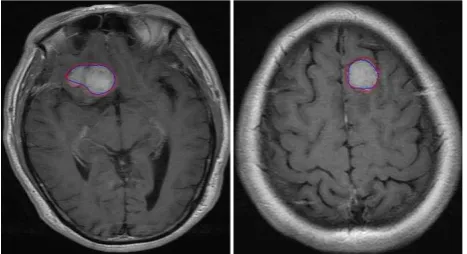
The data acquired at Southern Medical University was used to test the proposed algorithm for brain tumour segmentation. The examples of the tumour segmentation are presented in Figure 14.

Figure 14. Segmentation of the brain tumour performed by the proposed algorithm (blue) and manual delineation (red)

To estimate the accuracy and processing time of the brain tumour segmentation, we used a dataset included 200 slices. The results describing the quantitative metrics of the algorithm are shown in Table 5, Table 6 and Figure 15. Table 5 confirms the value of the angle (number of rays) does not significantly affect the accuracy of the algorithm for the regions of circular shape.

/4 /8 /16 /32

Mean±STD, % 82.2±11.8 83.0±11.4 82.5±11.6 82.7±11.2 Table 5. Brain tumour segmentation accuracy for different ∆

(number of rays)

Similarly to segmentation of the left ventricle, the average accuracy remains at a sufficiently high level in the brain tumour segmentation. The average accuracy value varies within 83%. The International Archives of the Photogrammetry, Remote Sensing and Spatial Information Sciences, Volume XLII-2/W12, 2019

Figure 15. Processing time of the brain tumour segmentation (in

milliseconds) of the proposed algorithm for different ∆

(number of rays)

/4 /8 /16 /32

Mean±STD, ms 5.1±1.1 6.9±1.4 11.8±4.2 16.0±3.0 Table 6. Processing time of the brain tumour segmentation for

different ∆ (number of rays)

The processing time of left ventricle segmentation strongly depends on the number of rays and the image dimensions. Such a tendency can be observed when comparing processing time for the heart segmentation (Figure 13) and the brain tumour segmentation (Figure 15).

5. DISCUSSION

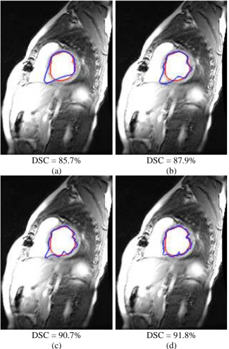
An important feature of the algorithm is an opportunity to obtain a relatively high level of accuracy varying ∆ and, hence, the number of emitted rays. For instance, Figure 16 and Figure 17 reflect two extreme cases for obtaining a good quality of segmentation. The algorithm can provide the best accuracy using

different angle change ∆ . Sometimes, a value of ∆ = /32 (64 rays) can provide a high level of segmentation. Such a case is reflected in Figure 17 for the left ventricle segmentation, where

the accuracy reached 91.8% with ∆ = /32. However, high

segmentation accuracy can be achieved with the relatively large

value of ∆ . For instance, brain tumour segmentation accuracy

of 89.0% was obtained using ∆ = /4 and is depicted in Figure 16. Sufficiently high accuracy of the algorithm was achieved due to the relatively simple shape of the regions under examination. When an object has a more complex, curved shape, the accuracy may have a lower value of the Dice similarity coefficient. To avoid this issue, the number of emitted rays should be increased significantly. But the main restriction of the proposed algorithm is the object shape. Objects with sophisticated non-convex shape will probably be segmented improperly or inaccurately. In this regard, this algorithm is better to apply to convex and closed objects. However, many organs of the human’s body have an elliptical or circular elongated shape. This allows the proposed algorithm to be applied to brain, lung, liver and heart segmentation.

One of the important features of the proposed algorithm is its scalability. The latter means that several algorithms can be used for border detection. We used the ensemble-based classifiers. As an additional method, one-dimensional neural networks can also be applied. Another key feature of the algorithm is an opportunity to use it for three-dimensional imaging. The latter can be solved using a spherical or cylindrical coordinate system.

DSC = 89.0% (a)

DSC = 81.1% (b)

DSC = 82.3% (c)

DSC = 80.4% (d)

Figure 16. Brain tumour segmentation with different ∆ : /4

(a), /8 (b), /16 (c) and /32 (d)

DSC = 85.7% (a)

DSC = 87.9% (b)

DSC = 90.7% (c)

DSC = 91.8% (d)

Figure 17. Heart segmentation with different ∆ : /4 (a), /8

(b), /16 (c) and /32 (d) The International Archives of the Photogrammetry, Remote Sensing and Spatial Information Sciences, Volume XLII-2/W12, 2019

According to the obtained results of segmentation (Table 3 and Table 5), there is a tendency of large spread for accuracy values. Such spread is related to the ray generation. The first ray of any object is always propagated in the same direction, not considering the features of the contour. If the first and subsequent rays fall into recesses or cavities of the contour, the accuracy of the contour decreases significantly. This disadvantage can be compensated by increasing the number of emitted rays. However, the random nature of the rays and their detachment from the peculiar properties of the contour are the drawbacks of the algorithm. A ray, falling into the contoured gap, deforms the resulting contour and reduces the final segmentation accuracy. It should be also noted the position of the initial point is important for the algorithm. When the starting point falls into a convex ejection, the accuracy of the algorithm decreases. This problem can partly be solved by increasing the number of generated rays. Ideally, the initial point should lie within the center of mass of the object.

6. CONCLUSION

The proposed algorithm is devoted to the segmentation of medical images. The algorithm assumes emitting rays to detect border pixels lying on the rays. Thus, the task is reduced to one-dimensional operations, which allows segmentation to be performed faster. The algorithm was tested on the cardiac MRI dataset consisting of 156 MRI images and brain tumour dataset consisting of 200 MRI images. The cardiac dataset included three patients with different diagnoses including Marfan syndrome, severe aortic insufficiency and a patient with no cardiac disorders. In turn, the brain tumour dataset included patients with meningioma, glioma, and a pituitary tumour. The highest similarity Dice coefficients for the heart and brain tumour segmentation, equal to 86.5±6.9% and 89.5±6.7% respectively, were achieved by the proposed algorithm. Regarding the processing time for this study, we have established that the relationship between processing time and the number of rays is quasi-proportional. The lowest processing time for the heart and the brain tumour segmentation, equal to 4.1±2.3 ms and 5.1±1.1 ms per slice respectively, were reached with 8 emitted rays. In addition, the algorithm can be accelerated using GPU-based computing because ray data processing can be performed in parallel.

ACKNOWLEDGEMENTS

This study was supported by the Russian Federation

Governmental Program ‘Nauka’ 12.8205.2017/ (additional number: 4.1769. .2017).

REFERENCES

Andreopoulos, A., Tsotsos, J.K., 2008. Efficient and generalizable statistical models of shape and appearance for analysis of cardiac MRI. Med. Image Anal. 12, 335–357. https://doi.org/10.1016/j.media.2007.12.003

Ayed, I. Ben, Chen, H., Punithakumar, K., Ross, I., Li, S., 2010. Graph cut segmentation with a global constraint: Recovering region distribution via a bound of the Bhattacharyya measure, in: 2010 IEEE Computer Society Conference on Computer Vision

and Pattern Recognition. IEEE, pp. 3288–3295.

https://doi.org/10.1109/CVPR.2010.5540045

Chawla, N. V., Lazarevic, A., Hall, L.O., Bowyer, K.W., 2010. SMOTEBoost: Improving Prediction of the Minority Class in

Boosting 107–119. https://doi.org/10.1007/978-3-540-39804-2_12

Cheng, J., Huang, W., Cao, S., Yang, R., Yang, W., Yun, Z., Wang, Z., Feng, Q., 2015. Enhanced performance of brain tumor classification via tumor region augmentation and partition. PLoS One 10. https://doi.org/10.1371/journal.pone.0140381

Cheng, J., Yang, W., Huang, M., Huang, W., Jiang, J., Zhou, Y., Yang, R., Zhao, J., Feng, Y., Feng, Q., Chen, W., 2016. Retrieval of Brain Tumors by Adaptive Spatial Pooling and Fisher Vector

Representation. PLoS One 11.

https://doi.org/10.1371/journal.pone.0157112

Cremers, D., Rousson, M., Deriche, R., 2007. A Review of Statistical Approaches to Level Set Segmentation: Integrating Color, Texture, Motion and Shape. Int. J. Comput. Vis. 72, 195– 215. https://doi.org/10.1007/s11263-006-8711-1

Danilov, V. V., Skirnevskiy, I.P., Gerget, O.M., Shelomentcev, E.E., Kolpashchikov, D.Y., Vasilyev, N. V., 2018. Efficient workflow for automatic segmentation of the right heart based on 2D echocardiography. Int. J. Cardiovasc. Imaging 34, 1–15. https://doi.org/10.1007/s10554-018-1314-4

Danilov, V. V, Skirnevskiy, I.P., Gerget, O.M., 2017. Segmentation of anatomical structures of the heart based on

echocardiography. J. Phys. Conf. Ser. 803, 1–6.

https://doi.org/10.1088/1742-6596/803/1/012031

Dey, J., Pan, T., Choi, D.J., Robotis, D., Smyczynski, M.S., Pretorius, P.H., King, M.A., 2009. Estimation of cardiac respiratory-motion by semi-automatic segmentation and registration of non-contrast-enhanced 4D-CT cardiac datasets, in: IEEE Transactions on Nuclear Science. pp. 3662–3671. https://doi.org/10.1109/TNS.2009.2031642

Galar, M., Fernandez, A., Barrenechea, E., Bustince, H., Herrera, F., 2012. A Review on Ensembles for the Class Imbalance Problem: Bagging-, Boosting-, and Hybrid-Based Approaches. IEEE Trans. Syst. Man, Cybern. Part C (Applications Rev. 42, 463–484. https://doi.org/10.1109/TSMCC.2011.2161285

Gorelick, L., Schmidt, F.R., Boykov, Y., Delong, A., Ward, A., 2012. Segmentation with Non-linear Regional Constraints via Line-Search Cuts, in: Lecture Notes in Computer Science (Including Subseries Lecture Notes in Artificial Intelligence and

Lecture Notes in Bioinformatics). pp. 583–597.

https://doi.org/10.1007/978-3-642-33718-5_42

Herbulot, A., Jehan-Besson, S., Duffner, S., Barlaud, M., Aubert, G., 2006. Segmentation of Vectorial Image Features Using Shape Gradients and Information Measures. J. Math. Imaging Vis. 25, 365–386. https://doi.org/10.1007/s10851-006-6898-y

Hu, L., Ji, Y., Li, Y., Gao, F., 2010. SAR image segmentation based on Kullback-Leibler distance of edgeworth, in: Lecture Notes in Computer Science (Including Subseries Lecture Notes in Artificial Intelligence and Lecture Notes in Bioinformatics). pp. 549–557. https://doi.org/10.1007/978-3-642-15702-8_50

Junmo Kim, Fisher, J.W., Yezzi, A., Cetin, M., Willsky, A.S., 2005. A nonparametric statistical method for image segmentation using information theory and curve evolution. IEEE Trans. Image

Process. 14, 1486–1502.

https://doi.org/10.1109/TIP.2005.854442

Katatbeh, Q., Martínez-Aroza, J., Gómez-Lopera, J., Blanco-The International Archives of the Photogrammetry, Remote Sensing and Spatial Information Sciences, Volume XLII-2/W12, 2019

Navarro, D., 2015. An Optimal Segmentation Method Using Jensen–Shannon Divergence via a Multi-Size Sliding Window

Technique. Entropy 17, 7996–8006.

https://doi.org/10.3390/e17127858

Lee, E.T.Y., 1989. Choosing nodes in parametric curve

interpolation. Comput. Des. 21, 363–370.

https://doi.org/10.1016/0010-4485(89)90003-1

Lee, S.U., Yoon Chung, S., Park, R.H., 1990. A comparative performance study of several global thresholding techniques for segmentation. Comput. Vision, Graph. Image Process. 52, 171– 190. https://doi.org/10.1016/0734-189X(90)90053-X

Li, L., Ross, P., Kruusmaa, M., 2013. Ultrasound image segmentation by Bhattacharyya distance with Rayleigh distribution, in: Signal Processing: Algorithms, Architectures, Arrangements, AND Applications. pp. 149–153.

Lu, Y., Cheung, Y., Tang, Y.Y., 2016. Hybrid Sampling with Bagging for Class Imbalance Learning, in: Journal of Physics A:

Mathematical and Theoretical. pp. 14–26.

https://doi.org/10.1007/978-3-319-31753-3_2

Lynch, M., Ghita, O., Whelan, P.F., 2008. Segmentation of the left ventricle of the heart in 3-D+ t MRI data using an optimized nonrigid temporal model. Med. Imaging, IEEE Trans. https://doi.org/10.1109/TMI.2007.904681

Ng, H.P., Ong, S.H., Foong, K.W.C., Goh, P.S., Nowinski, W.L., 2006. Medical Image Segmentation Using K-Means Clustering and Improved Watershed Algorithm, in: IEEE Southwest Symposium on Image Analysis and Interpretation. IEEE, pp. 61– 65. https://doi.org/10.1109/SSIAI.2006.1633722

Noble, J.A., Boukerroui, D., 2006. Ultrasound image segmentation: a survey. IEEE Trans. Med. Imaging 25, 987– 1010. https://doi.org/10.1109/TMI.2006.877092

Pham, D.L., Xu, C., Prince, J.L., 2000. Current Methods in Medical Image Segmentation. Annu. Rev. Biomed. Eng. 2, 315– 337. https://doi.org/10.1146/annurev.bioeng.2.1.315

Pizer, S.M., Amburn, E.P., Austin, J.D., Cromartie, R., Geselowitz, A., Greer, T., ter Haar Romeny, B., Zimmerman, J.B., Zuiderveld, K., 1987. Adaptive histogram equalization and its variations. Comput. Vision, Graph. Image Process. 39, 355– 368. https://doi.org/10.1016/S0734-189X(87)80186-X

Reyes-Aldasoro, C.C., Bhalerao, A., 2006. The Bhattacharyya space for feature selection and its application to texture

segmentation. Pattern Recognit. 39, 812–826.

https://doi.org/10.1016/J.PATCOG.2005.12.003

Sankur, B., 2004. Survey over image thresholding techniques and quantitative performance evaluation. J. Electron. Imaging 13, 146. https://doi.org/10.1117/1.1631315

Seiffert, C., Khoshgoftaar, T.M., Van Hulse, J., Napolitano, A., 2010. RUSBoost: A hybrid approach to alleviating class imbalance. IEEE Trans. Syst. Man, Cybern. Part ASystems

Humans 40, 185–197.

https://doi.org/10.1109/TSMCA.2009.2029559

Wang, S., Yao, X., 2009. Diversity analysis on imbalanced data sets by using ensemble models. 2009 IEEE Symp. Comput.

Intell. Data Mining, CIDM 2009 - Proc. 324–331.

https://doi.org/10.1109/CIDM.2009.4938667

The International Archives of the Photogrammetry, Remote Sensing and Spatial Information Sciences, Volume XLII-2/W12, 2019