Solution strategies for a supply chain deterministic model

Rochester Institute of Technology

RIT Scholar Works

Theses Thesis/Dissertation Collections

3-1-2007

Solution strategies for a supply chain deterministic

model

Ming Hong

Follow this and additional works at:http://scholarworks.rit.edu/theses

This Thesis is brought to you for free and open access by the Thesis/Dissertation Collections at RIT Scholar Works. It has been accepted for inclusion in Theses by an authorized administrator of RIT Scholar Works. For more information, please [email protected].

Recommended Citation

Rochester Institute of Technology

Solution Strategies

For

A Supply Chain Deterministic Model

A Thesis

Submitted in partial fulfillment of the requirements for the degree of

Master of Science in Industrial Engineering

In the

Department of Industrial and Systems Engineering

Kate Gleason College of Engineering

By

Ming Hong

MS, IE candidate

Acknowledgements

The successful completion of this thesis is a result of input from numerous

contributors, and I would like to thank each and every one of them. I am grateful for all the

resources and support provided to me by Department of Industrial and Systems Engineering.

I would especially like to thank my advisor and mentor Dr. Moises Sudit for the

direction and support he has provided along the way. He has given me valuable insight and an

intuitive view on the behavior of mathematical models, as well provided me with knowledge

and tools required to solve the model. His constant guidance kept me on track and moving

towards achieving my goals.

I would also like to thank my committee members, Dr. Andres Carrano and Dr. Brian

Thorn, for their help in carefully reviewing my thesis and providing feedback. Both have been

a tremendous help.

Last but not the least; I want to thank my family and friends for their continuous

Committee Members:

Dr. Moises Sudit

Associate Adjunct Professor, Director of Business Development Industrial and Systems Engineering Department

Rochester Institute of Technology

Dr. Andres Carrano

Associate Professor

Industrial and Systems Engineering Department Rochester Institute of Technology

Dr. Brian Thorn

Associate Professor

Industrial and Systems Engineering Department Rochester Institute of Technology

Approved By:

Dr. Moises Sudit _____________________________ Date ___________

Dr. Andres Carrano _____________________________ Date ___________

Abstract

To most firms, intelligent supply chain decisions are essential to achieve

competitiveness in an environment characterized with increasing globalization and relentless

changes. As the supply chain concept largely evolved from traditional logistics management,

practitioners and researchers have historically focused on the individual processes of a supply

chain. A wide array of mathematical models have been developed to tackle such functional

issues as inventory level, lead-time performance, delivery performance, customer satisfaction

and so on. This research presents a model that aims to evaluate and optimize the overall

performance of the supply chain. The key nodes and variables in the model are composed of

plant location and production volume, storage location and volume, transportation mode and

volume. Optimization of the model is to minimize the total supply chain operation cost,

expressed as the sum of production cost, storage cost, transportation cost and lost-sale cost.

Our methodology is a three-phased approach. First, we build a mixed integer-programming

model of 3-tier supply chain with plant, warehouse, and retailer,

multi-period and restricted capacity. This mathematical model is solved by CPLEX/OPL. Due to

excessive computation time to reach the Optimal Solution, we introduce the second phase to

develop heuristic solutions to reduce the computation time. In the final phase, we evaluate the

proposed heuristic solutions. Result analysis shows that the computation time is generally

exponentially correlated to the data size in seeking Optimal Solutions, whereas it generally

follows the polynomial distribution when the Heuristic Solutions are applied. Consequently,

TABLE OF CONTENTS

1 INTRODUCTION ...5

2 LITERATURE REVIEW ...7

3 SCOPE AND SOLUTION STRATEGY ...12

3.1 SCOPE... 12

3.2 SOLUTION APPROACH... 13

3.2.1 Build Mixed Integer Programming Model ... 13

3.2.1.1 Model Assumptions... 14

3.2.1.2 Model Indexes ... 15

3.2.1.3 Model Decision variables ... 16

3.2.1.4 Model Coefficients ... 16

3.2.1.5 Model Constraints ... 17

3.2.1.6 Model Objective ... 19

3.2.2 Solve Model in CPLEX/OPL ... 20

3.2.3 Issue with Mixed Integer Model in CPLEX/OPL ... 21

4 HEURISTIC DEVELOPMENT ...23

4.1 HEURISTIC SOLUTION I... 23

4.2 HEURISTIC SOLUTION IRESULT... 26

4.3 ISSUE WITH HEURISTIC I ... 29

4.4 HEURISTIC SOLUTION II ... 30

4.5 HEURISTIC SOLUTION IIRESULT... 33

4.6 HEURISTIC SOLUTION II VS.OPTIMAL SOLUTION AND HEURISTIC SOLUTION I ... 36

5 RESULT ANALYSIS ...38

5.1 PAIRED T-TEST... 38

5.2 ONE –SAMPLE T-TEST ANALYSIS... 41

6 CONCLUSION & FUTURE RESEARCH ...49

7 BIBLIOGRAPHY...54

APPENDIX A: MIXED INTEGER MODEL IN CPLEX ...60

APPENDIX B : OPL SCRIPT FOR HEURISTIC SOLUTION I ...67

1

Introduction

A supply chain is a network of facilities and distribution options that performs the

functions of procurement of materials, transformation of these materials into intermediate and

finished products, and the distribution of these finished products to customers.

Supply chain management calls for understanding the complex interactions among

individual flows, functions and stages within the supply chain, and based on that

understanding, maximizing the overall supply chain performance and profitability.

Traditionally, distribution, planning, manufacturing, marketing and transportation operate

independently. Functional objectives are often conflicting with each other at the best. For

instances, marketing objectives of brand recognition and reputation through discreet designs,

on-demand delivery, or impeccable customer service are invariably in conflict with

manufacturing goals of smooth process and scale economy through mass production and

distribution. Many manufacturing operations are designed to maximize throughput and lower

costs with less consideration for the impact on inventory levels and distribution capabilities.

Clearly, the design and management of these processes and functions determines whether the

supply chain would meet its requisite performance objectives. This study assumes a total

supply chain strategy on which our mathematic models are developed and calibrated to

achieve overall optimization.

The supply chain is a dynamic system. Not only does the demand fluctuates over time,

but also production cost, logistics cost, capacity change from time to time. For instance, the

crude oil price has increased drastically in last 5 years and transportation cost is typically

chain partner operating at low cost due to labor condition or land use in distant sites or foreign

countries may lose its advantage after the increased transportation cost breaks the balance.

Therefore, to truly optimize supply chain performance over time, specific characteristics of

cost for each period of time should be calculated. However, certain supply chain dynamics,

such as demand fluctuation, production uncertainty and transportation instability, are omitted

in most mathematical models. Our research develops a generic model to address the dynamics

of supply chain configuration.

In this paper, we propose a high level holistic model for an integrated dynamic supply

chain with multi-input/multi-output. The mixed integer programming models is built in

CPLEX/OPL to minimize the total supply chain cost. Due to the often disparate goals of

individual functions and processes within the supply chain and complexity of modeling

constrains and value boundaries, finding an optimal equilibrium for the entire supply chain

can be a serious challenge. Computational Complexity Theory categorizes most of these

problems as NP-Hard, which makes optimal solutions unattainable. We address this issue by

applying stepwise heuristic solutions such that CPLEX/OPL solves a model with fairly large

2

Literature Review

The topic of supply chain modeling and analysis has been of great interest, from practical

and research perspectives, due to its importance in the competitive environment of

present-day global economy.

The body of literature on supply chain configuration design is vast and keeps growing

over the last two decades. Geoffrion and Graves (1974) initiated one of the earliest works.

They introduce a commonly occurring problem in distribution system design, which is the

optimal location of intermediate distribution facilities between plants and customers. A

multi-commodity capacitated single-period version of this problem is formulated as a mixed integer

linear program. A solution technique based on Benders Decomposition is developed,

implemented, and successfully applied to a real problem for a major food firm with 17

commodity classes, 14 plants, 45 possible distribution center sites, and 121 customer zones.

A succession of papers by Cohen and Lee address a variety of issues of supply chain

network design. Cohen and Lee (1988) present a comprehensive model framework for linking

decisions and performance throughout the material-production-distribution supply chain. The

purpose of the model is to support analysis of alternative manufacturing material/ service

strategies. A series of linked, approximate sub-models and a heuristic optimization procedure

are introduced. Cohen and Lee (1989) developed a normative model for resource deployment

decisions in a global manufacturing and distribution network. This model can be used to

support analysis of global manufacturing policies. Its constraints include facility capacity,

regional demand requirements, material balance, and government offset requirements. The

distribution, and transportation. Lee and Billington (1995) validate these models by applying

it to analyze the global manufacturing strategies of Hewlett-Packard. The paper gives details

of Hewlett Packard's experiences. Lee and Kim (2000, 2002) develop an analytical model to

solve the integrated production-distribution problems in supply chain management. They

propose a hybrid approach combining the analytic and simulation model for multi-product,

multi-period problems at strategic level. Operation time in the analytic model is considered as

a dynamic factor. They obtain the more realistically optimal production-distribution plans for

the integrated supply chain system reflecting stochastic natures by performing the iterative

hybrid analytic-simulation procedure.

Tremendous practical research has been done in the area of integrating the supply chain

system in recent years. Integration involves the joint decision making among the producer, the

distributors and the retailers. The success experiences of National Semiconductor, Wal-Mart,

and Procter & Gamble have demonstrated that integrating the supply chain has significantly

influenced the company’s performance and market share (Simchi-Levi et al. 2001). Yang and

Wee (2000) develop an economic ordering policy of a deteriorating item with a constant

production and demand rate. By considering the view of both of the vendor and buyer, a

mathematical model subject to single-vendor-single-buyer and multiple deliveries per order is

developed. It can be shown that the integrated approach results in an impressive

cost-reduction compared with an independent decision by the buyer. Jack et al. (2000) presents a

method for modeling the dynamic behavior of food supply chains and evaluating alternative

designs of the supply chain by applying discrete-event simulation. Its modeling method is

based on the concepts of business processes, design variables at strategic and operational

transportation and infinite horizon multi-echelon inventory cost function. It considers the

trade-off between inventory cost, direct shipment cost, and facility location cost in such a

system. The problem is to determine how many warehouses to set up, where to locate them,

how to serve the retailers using these warehouses, and to determine the optimal inventory

policies for the warehouses and retailers. The objective is to minimize the total multi-echelon

inventory, transportation, and facility location costs. They structure this problem as a

set-partitioning integer-programming model and solve it using column generation. More recently,

Iida (2002) present a non-stationary periodic review dynamic production-inventory model

with uncertain production capacity and uncertain demand. The maximum production capacity

varies stochastically. Wee and Yang (2002) derives an optimal solution by revising Goyal's

model. A heuristic solution model is also developed for a producer-distributors-retailers

inventory system using the principle of strategic partnership. Numerical results indicate the

heuristic solution is a good estimation of the optimal solution.

Most existing studies assume a single transportation mode with a fixed lead-time. Matta

and Miller (2002) study the problem of coordinating production and transportation scheduling

decisions, in particular, how changes in plant capacity and costs affect the coordination of

scheduling decisions as well as the choice of transportation modes and carriers. They

formulate the problem as a mixed integer-programming model and use a solution procedure

that exploits the underlying structure of our problem. The result shows that coordinated

schedules yield significant cost savings resulting from the modest use of the expensive fast

transport mode, coordinated product changeovers.

For supply chain optimization practitioners, one major obstacle is related to supply chain

computationally intractable. Ding, Benyoucef and Xie (2004) present a simulation-based

optimization method for multi-criteria production-distribution network design. The method

consists of a multi-objective optimizer and a simulation module. The uniqueness of their

proposed method is that it not only performs multi-objective optimization, but more

importantly it optimizes supply chain structure and addresses each configuration’s operational

performances. Stochastic facts along the whole supply chain (demand fluctuation,

transportation uncertainty, etc.) are taken into account during the optimization process.

Moreover, it enables the optimization of qualitative parameters.

Computational Complexity Theory categorized most of mixed integer programming

problems as NP-Hard, which makes optimal solutions unattainable. Their exact methods are

impractical for real problems. Most researchers attempted to find effective heuristic or

approximate approaches. Chu and Chen (2003) developed a heuristic approach that combines

Lagrangian Relaxation (LR) with local improvement for supply chain planning modeled as a

multi-item multi-level capacitated lot-sizing problem. They explored some structural

properties of the problem and improve the approach by reducing the number of Lagrangian

multipliers. As the previous one, their new LR approach only relaxes the technical constraints

that each 0-1-setup variable is positive. By taking the advantages of the reduced number of

the multipliers, the new approach can obtain solution of the same high quality with reduced

computation time.

A supply chain consists of complicated operations and relationships, and its analysis

requires a carefully defined approach. Supply chain modeling can be overwhelming due to

sheer amount of data and structural complexity. On the other hand, it is also possible to

the supply chain. This research presents the development of a high-level supply chain model.

A mixed integer programming model is developed for a Plant-Distribution-Retailer chain with

the consideration of uncertain capacity, uncertain demand, uncertain production cost,

uncertain storage cost and transportation modes and lead time. Heuristic approaches are

presented to solve the model within computationally acceptable timeframe. Data analysis is

3

Scope and Solution Strategy

The following sections in this chapter explain the scope of the research, methodologies

employed, and the integer-programming to be used for problem solving.

3.1 Scope

The objective of this research is to develop and solve a deterministic analytical model

that minimizes the cost of the total supply chain operation, by considering manufacturing cost,

transportation cost, storage cost and backorder cost. In so doing, the research results can be

applied to determine the optimal supply chain configuration, for any given cost, capacity

demand and lead time metrics.

There are 3 types of multi-locations included in this research: plants, warehouses and

retailers.

• Plant: Plants are the upstream of the chain. Its functionality is making finish

goods. In this research, it’s assumed that there is no inventory stored at any

plant. Whatever produced is shipped out at the end of each time period.

• Warehouse: Warehouses do the transshipments. It receives, stores and ships

products. The same items come in that go out, and are not transformed.

• Retailers: Retailers are the downstream of the chain. It stores and distributes the

products and is the point where products are consumed

Transportation is a very important factor in our configuration; both its lead-time and its

3.2 Solution Approach

The solution methodology consists of developing and analyzing the mathematical

model in three phases. Phase 1, an integer-programming model is developed, and therefore

defines the problem and research scope. To improve the computational efficiency, the

heuristic solution would be mathematically developed in Phase 2. A series of experiments

will be conducted in Phase 2. In Phase 3, the performance of the proposed heuristic is

evaluated to demonstrate its advantage.

3.2.1 Build Mixed Integer Programming Model

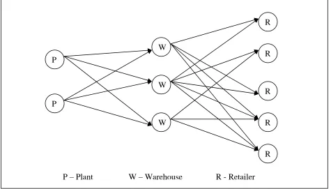
Figure 1 shows a typical supply chain network. The configuration of this network is

based on determination of:

(i) Locations and production volume for Ps;

(ii) Locations and production volume for Ws

(iii) Locations and production volume for Rs;

(iv) Transportation mode volume between Ws and Rs;

P

W

W W

R R R R R

P

P – Plant W – Warehouse R - Retailer

Figure 3.1: Structure of Typical Supply Chain Network

3.2.1.1 Model Assumptions

The following are the assumptions made in the formulation:

• Three facility levels: plants, warehouses and retailers;

(Mitigation: more layers can always be added and won’t structurally change the

configuration)

• At each location step and each transportation step, only 1 cost coefficient is

applied which includes all the cost incurring while operating this step

(Mitigation- aggregation of all costs into one is practical)

(Mitigation - similar consideration of inventory at warehouse could be extended

to plant)

• No backorder happening at Plants and Warehouses

(Mitigation: similar consideration of backorder cost at retailers could be

extended to warehouses and plants)

• Only one product is considered

(Mitigation - we could talk about generic shipment units)

• No upper bound for transportation amount

(Mitigation – make an artificial mode with a “Huge” cost)

• No Setup cost considered

(Mitigation – fixed-cost problem adds complexity)

• One shipment order has to go on the same mode

(Mitigation –cost will increase, but it can be done manually)

3.2.1.2 Model Indexes

• i = index for Plant ( i = 1,2,3……I )

• j = index for Warehouse (j = 1,2,3……J)

• k = index for Retailer (k= 1,2,3……K)

• m = modes of transportation combined with transportation volume level

Low/Med/High

(m = airL, airM, airH, seaL, seaM, seaH, railL, railM, railH, truckL, truckM, truckH)

3.2.1.3 Model Decision variables

Decision variables are used to completely define the problem.

• p

it

X = Amount of products produced at Plant i at time t

• X_ijmt = Amount of products transported from Plant i to Warehouse j by transport

mode m at time t

• W_ijmt = 1 if products transported from Plant i to Warehouse j by mode m at time t; 0,

otherwise.

• w

jt

X = Amount of products stored at Warehouse j at time t

• Y_jkmt = Amount of products transported from Warehouse j to Retailer k by transport

mode m at time t

• U_jkmt = 1 if of products transported from Warehouse j to Retailer k by mode m at

time t; 0, otherwise.

• R

kt

X = Amount of products stored at Retailer k at time t

• Z_kt = 1 if there is back order at Retailer k at time t; 0, otherwise.

• B_kt = Back order quantity at Retailer k at time t

3.2.1.4 Model Coefficients

• PCit = Production cost at Plant i at time t, $ per unit

• TC_ijmt = Transportation cost from Plant i to Warehouse j at time t via transport mode

• WC_jt = Storage cost at Warehouse j at time t, $ per unit

• TCjkmt = Transportation cost from Warehouse j to Retailer k at time t via transport

mode m, $ per Unit

• RCkt = Storage cost at Retailer k at time t, $ per unit

• LCkt = Backorder cost at Retailer k at time t, $ per unit

• T_ijm = Transportation time from Plant i to Warehouse j via transport mode m

• T_jkm = Transportation time from Warehouse j to Retailer k via transport mode m

• Lit = Production limit of Plant i at time t

• L_jt= Storage limit of Warehouse j at time t

• Lkt = Storage limit of Retailer k at time t

• D_kt= Demand at Retailer k at time t

• w

j

INV ₀ = Starting inventory at Warehouse j

• R

k

INV ₀ = Starting inventory at Retailer k

• TL_m = Lower bound of transportation volume via mode m

• TU_m = Upper bound of transportation volume via mode m

• M = a large natural number

3.2.1.5 Model Constraints

1. The volume produced at Plant i can’t exceed its capacity limit at time t

t i L

The amount of products transported from each plant i to all warehouse j at time t via

all transport modes is equal to the production volume at plant i at time t for all plant i

t i X X _ijmt m j p

it =

∑

∑

2. The amount of products transported from each plant i to each warehouse j at time t via

mode m is within the volume limit of this mode

t m j i W TU X W

TLm* ijmt ≤ ijmt ≤ m* ijmt ∀, , ,

3. The inventory at warehouse j at time t is equal to the inventory at warehouse j at time

t-1 plus the products transported to j from all i at time t minus the products transported

from j to all k at time t

t j Y X X X jkmt m k Tijm t ijm m i w jt w

jt = −1 +

∑

∑

∑

∑

The inventory at Warehouse j at time 0 is equal to the starting inventory

t j INV X w j w

j0 = 0 ∀,

The inventory at Warehouse j at time t can’t exceed its capacity limit at time t

t j L

X jt

w

jt ≤ ∀,

4. The amount of products transported from each warehouse j to each retailer k at time t

via mode m is within the volume limit of this mode

t m k j U TU Y U

TL_m* _jkmt ≤ _jkmt ≤ _m* _jkmt ∀, , ,

5. The inventory at Retailer k at time t is equal to the inventory at retailer k at time t-1

plus the products transported to k from all j at time t minus the back order of k at time

t k B D B Y X

X _{jkmt Tjkm kt kt kt}

m j R kt R

kt = −1 +

∑

∑

If there is back order at Retailer k at time t, the ending inventory at k at time t is equal

to Zero.

t k Z

M

X_ktR ≤ *(1− _ktR) ∀ ,

If there is no back order at Retailer k at time t, the back order quantity at k at time t is

equal to Zero

t k Z

M

Bkt ≤ * ktR ∀ ,

The inventory at Retailer k at time 0 is equal to the starting inventory

k INV

X kR

R

k0 = 0 ∀

The inventory at Retailer k at time t can’t exceed its capacity limit at time t

t k L

X kt

R

kt ≤ ∀ ,

6. Xitp, Xijmt, w jt

X , Y_jkmt , X_ktR, B_kt, Z_kt, W_ijmt, U_jkmtare non-negative integer

3.2.1.6 Model Objective

Total production cost occurred at all plants locations (i) in time period t:

it p it i PC X *

∑

Total transportation cost from all plants locations (i) to all warehouse locations

(j) using all transportation modes (m) in time period t: _{ijmt ijmt}

m j i TC X *

∑

∑

∑

Total storage cost occurred at all warehouse locations (j) in time period t:

Total transportation cost from all warehouse locations (j) to all retailer

locations (k) using all transportation modes (m) in time period t:

jkmt jkmt m k j TC Y *

∑

∑

∑

Total storage cost occurred at all retailer locations (k) in time period t:

kt R kt k RC X *

∑

Total back order cost occurred at all retailer locations (k) in time period t:

kt kt k LC B *

∑

Therefore, the objective function of this model that minimizes the total supply

chain cost (the sum of production cost, storage cost, transportation cost and backorder

cost) is: Minimize: jkmt jkmt m k j jt w jt j ijmt ijmt m j i it p it i t TC Y WC X TC X PC

X * * * *

(

∑

∑

∑

∑

∑

∑

∑

∑

∑

) *

* _{kt kt}

k kt R kt k LC B RC X

∑

∑

3.2.2 Solve Model in CPLEX/OPL

Programming it into ILOG CPLEX 9.0 tests the feasibility of the proposed model. We

write the programming codes for the mixed integer model in CPLEX, which is attached in

APPENDIX A. Considering the amount of time required to solve the model in CPLEX, we

and 6 transportation modes. The feasible optimal solution for the small data model is

calculated within 1 second. (All the applications in this research are run on the computer with

1.0G RAM)

3.2.3 Issue with Mixed Integer Model in CPLEX/OPL

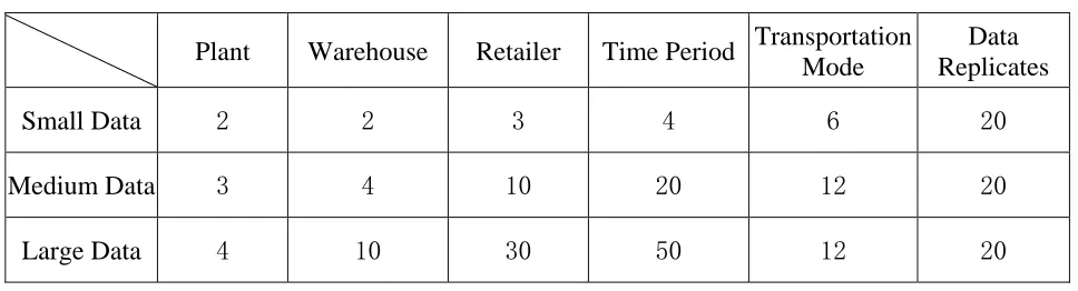
With increased data sizes, the model computation time increases correspondingly. We

categorize the data sets as “Large”, “Medium”, and “Small” size. All the coefficient data are

randomly generated out of MATLAB.

Table 3.1 Model Data Size

Plant Warehouse Retailer Time Period Transportation

Mode

Data Replicates

Small Data 2 2 3 4 6 20

Medium Data 3 4 10 20 12 20

Large Data 4 10 30 50 12 20

“Small” model consists of 2 plants, 2 warehouses, 3 retailers, 4 time periods and 6

transportation modes. The average running time for the small model is less than 1 second.

“Medium” model consists of 3 plants, 4 warehouses, 10 retailers, 20 time periods and 12

transportation modes. The running time for the medium model varies from 5 seconds to 3

minutes depending on the data. Its average is about 1 minute.

“Large” model consists of 4 plants, 10 warehouses, 30 retailers, 50 time periods and 12

10 warehouses / 30 retailer distributions appears to be relatively practical size for the

contemporary real business. 50 time periods are set as 50 weeks for one year. 12

transportation modes are set for air, sea, train and truck at high / medium/low shipping size.

20 “Large” data sets are randomly generated in MATLAB. The running time of these data

sets is much longer than the “Small” data and “Medium” data, which vary from 8 hours to 22

hours. It takes averagely about 13 hours to complete solving the model, which is not

4

Heuristic Development

4.1 Heuristic Solution I

Ideally, the best solution of mixed integer mathematical model is its optimal solution.

However, the excessive running time makes it less practical and less appealing in the real

business world. In order to solve the problem in a reduced computation time, we introduce the

heuristic solutions.

We run Linear Models in CPLEX, whose decision variables are all set as non-integer.

For the same data size, the running time for Linear Model is much less than that of Mixed

Integer Model. Hence, the idea of the heuristic solution is to assume all the decision variables

to be non-integer, solve this linear model first within a small amount of time, and then force

the non-integer result to integer number as per some conditions. The goal of the heuristic

solution is to shorten the model solving time in CPLEX.

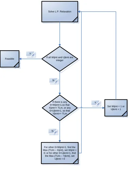
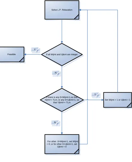
Heuristic Solution I is our first trial. The flow chart of the Heuristic Solution I is

shown as below in Figure 4.1.

1. Change the data type of all integer decision variables from integer to linear, solve

the linear model relaxation in CPLEX;

2. If all W_ijmt and U_jkmt are integer, then the result is feasible, we obtain the heuristic

solution;

* = 1 if products transported from Plant i to Warehouse j by mode

m at time t; 0, otherwise.

ijmt W

* = 1 if of products transported from Warehouse j to Retailer k

by mode m at time t; 0, otherwise

3. If any of W_ijmt are non-integer, and if there is any 0<W_ijmt<1, so that X_ijmt ≥ TL_m,

we set these W_ijmt = 1. If any of U_jkmt are non-integer, and if there is any

0<U_jkmt<1, so that Y_jkmt ≥ TL_m, we set these U_jkmt = 1.

4. For the rest of W_ijmt which is 0<W_ijmt<1, find out the Maximum (TU_m-X_ijmt), set

this W_ijmt = 0. For the rest of U_jkmt which is 0<U_jkmt<1, find out the Maximum

(TU_m-Y_jkmt), set this U_jkmt = 0.

5. Continue running the Linear Model until it yields feasible solution.

It takes hundreds of cycles to find the heuristic solution; therefore it becomes even

more time consuming if we change the data manually. We write OPL script to run the

heuristic solution automatically. The codes for Heuristic Solution I is attached in

Solve L.P. Relaxation

If all Wijmt and Ujkmt are integer

If there is any 0<Wijmt<1,so that Xijmt>= TLm, or any

0<Ujkmt<1, so that Yjkmt>= TLm

For other 0<Wijmt<1, find the Max.(TUm – Xijmt), set Wijmt =

0; or for other 0<Ujkmt<1, find the Max.(TUm – Yjkmt), set

Ujkmt = 0 Feasible

Set Wijmt = 1 or Ujkmt = 1 Y

N

Y

N

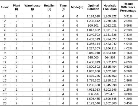
4.2 Heuristic Solution I Result

For consistency and later result comparison, we use the same data sets to run the

Heuristic Solution for all “Large”, “Medium” and “Small” size.

We run 20 “Small” data sets first. There is no large time difference between the optimal

solution running and heuristic solution running since the running time for both two is less

than 1 second, which is very short and could be ignored. The results are shown as below in

TABLE 4.1. We can see that the heuristic result is about 0.5% ~ 8% worse than the optimal

result.

Table 4.1 Result Comparison between Optimal and Heuristic I for Small Data Sets

Index Plant

(i) Warehouse (j) Retailer (k) Time

(t) Mode(m)

Optimal Solution Heuristic I Solution Result Difference Percentage

1 2 2 3 4 6 1,199,010 1,269,822 5.91%

2 2 2 3 4 6 1,238,612 1,270,634 2.59%

3 2 2 3 4 6 959,101 1,022,021 6.56%

4 2 2 3 4 6 1,047,602 1,071,014 2.23%

5 2 2 3 4 6 1,240,903 1,331,836 7.33%

6 2 2 3 4 6 1,402,313 1,424,627 1.59%

7 2 2 3 4 6 1,356,114 1,423,042 4.94%

8 2 2 3 4 6 1,217,303 1,266,211 4.02%

9 2 2 3 4 6 3,840,018 3,884,431 1.16%

10 2 2 3 4 6 935,000 964,808 3.19%

11 2 2 3 4 6 1,480,019 1,552,428 4.89%

12 2 2 3 4 6 2,800,503 2,815,404 0.53%

13 2 2 3 4 6 1,035,656 1,102,967 6.50%

14 2 2 3 4 6 1,465,285 1,526,453 4.17%

15 2 2 3 4 6 1,785,362 1,818,512 1.86%

16 2 2 3 4 6 1,250,320 1,345,298 7.60%

17 2 2 3 4 6 4,052,033 4,102,546 1.25%

18 2 2 3 4 6 856,256 925,475 8.08%

19 2 2 3 4 6 1,526,465 1,590,545 4.20%

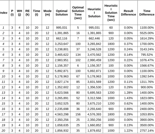
We then run 20 “Medium” data sets. The results are shown as below in TABLE 4.2.

We can see that the heuristic result is about 0.0% ~ 1.5% worse than the optimal result, which

is less damaged than the small data sets. However, the running time for the heuristic solution

is even much longer than that of the optimal solution. The sacrifice of the time varies from

800% ~ 5500%.

Table 4.2 Result Comparison between Optimal and Heuristic I for Medium Data Sets

Index P

(i) WH (j) RE (k) Time (t) Mode (m) Optimal Solution Optimal Solution Time (sec) Heuristic I Solution Heuristic I Solution Time (sec) Result Difference Time Difference

1 3 4 10 20 12 995,031 5 995,031 60 0.00% 1100.00%

2 3 4 10 20 12 1,391,865 16 1,391,865 900 0.00% 5525.00%

3 3 4 10 20 12 662,116 7 662,446 120 0.05% 1614.29%

4 3 4 10 20 12 3,253,647 100 3,265,842 1800 0.37% 1700.00%

5 3 4 10 20 12 3,238,801 37 3,246,528 1200 0.24% 3143.24%

6 3 4 10 20 12 3,465,622 134 3,470,562 1200 0.14% 795.52%

7 3 4 10 20 12 2,983,951 102 2,990,459 1200 0.22% 1076.47%

8 3 4 10 20 12 1,156,357 6 1,156,357 100 0.00% 1566.67%

9 3 4 10 20 12 5,892,871 100 5,892,871 1200 0.00% 1100.00%

10 3 4 10 20 12 5,178,963 67 5,178,963 1000 0.00% 1392.54%

11 3 4 10 20 12 3,827,174 85 3,831,569 1200 0.11% 1311.76%

12 3 4 10 20 12 1,352,602 12 1,356,530 120 0.29% 900.00%

13 3 4 10 20 12 5,623,566 80 5,695,563 1200 1.28% 1400.00%

14 3 4 10 20 12 3,265,891 52 3,312,566 1000 1.43% 1823.08%

15 3 4 10 20 12 3,652,525 80 3,675,210 1200 0.62% 1400.00%

16 3 4 10 20 12 2,235,698 36 2,255,640 900 0.89% 2400.00%

17 3 4 10 20 12 4,563,298 156 4,576,393 1800 0.29% 1053.85%

18 3 4 10 20 12 2,350,256 25 2,350,256 1000 0.00% 3900.00%

19 3 4 10 20 12 1,658,635 25 1,660,852 900 0.13% 3500.00%

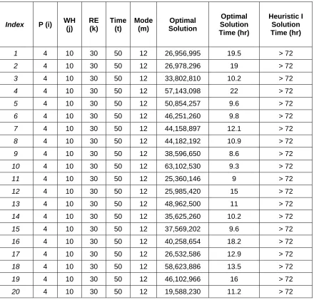
Finally, we run 20 “Large” data sets, which are the biggest bottleneck of optimal

solution running time. The results are shown as below in TABLE 4.3. Unfortunately, the

running time for the heuristic solution is much longer than that of the optimal solution. We are

not able to retrieve the solution even after 72 hours. We did not run all the models to the end

due to the time constrain.

Table 4.3 Result Comparison between Optimal and Heuristic I for Large Data Sets

Index P (i) WH (j) RE (k) Time (t) Mode (m) Optimal Solution Optimal Solution Time (hr) Heuristic I Solution Time (hr)

1 4 10 30 50 12 26,956,995 19.5 > 72

2 4 10 30 50 12 26,978,296 19 > 72

3 4 10 30 50 12 33,802,810 10.2 > 72

4 4 10 30 50 12 57,143,098 22 > 72

5 4 10 30 50 12 50,854,257 9.6 > 72

6 4 10 30 50 12 46,251,260 9.8 > 72

7 4 10 30 50 12 44,158,897 12.1 > 72

8 4 10 30 50 12 44,182,192 10.9 > 72

9 4 10 30 50 12 38,596,650 8.6 > 72

10 4 10 30 50 12 63,102,530 9.3 > 72

11 4 10 30 50 12 25,360,146 9 > 72

12 4 10 30 50 12 25,985,420 15 > 72

13 4 10 30 50 12 48,962,500 11 > 72

14 4 10 30 50 12 35,625,260 10.2 > 72

15 4 10 30 50 12 37,569,202 9.6 > 72

16 4 10 30 50 12 40,258,654 18.2 > 72

17 4 10 30 50 12 26,532,586 12.9 > 72

18 4 10 30 50 12 58,623,886 13.5 > 72

19 4 10 30 50 12 46,102,966 16 > 72

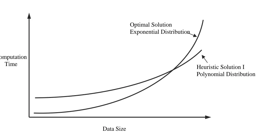
4.3 Issue with Heuristic I

Computation

Exponential Distribution Optimal Solution

Time _{Heuristic Solution I}

Polynomial Distribution

Data Size

Figure 4.2: Data Size vs. Computation Time (Optimal Solution & Heuristic Solution I)

As Figure 4.2 showed above, when we run Optimal Solution, the running time

exponentially increases with expanding of the data size. In contrast, it increases following the

polynomial distribution when we run Heuristic Solution.

The time constrain hasn’t be solved by Heuristic Solution I. The computation time for

Large Data is still not acceptable. And it is even much longer than the Optimal Model when

we run the Small data and Medium data. Therefore, we have to come up with another

Heuristic Solution. However, Heuristic Solution I only slightly impairs or distorts the solution

4.4 Heuristic Solution II

As noted above, Heuristic Solution I conducted earlier doesn’t distort the optimal

result significantly. The bottleneck of Heuristic Solution I is suspected as the running time to

force the fraction parameters to Zero only once each time. Heuristic Solution II is build up

onto Heuristic Solution I; however all fraction parameters are forced to Zero at one time.

The flow chart of the Heuristic Solution II is shown as below in Figure 4.3.

1. Change the data type of all integer decision variables from integer to linear,

solve the linear model relaxation in CPELX;

2. If all W_ijmt and U_jkmt are integer, then the result is feasible, we get the heuristic

solution;

* = 1 if products transported from Plant i to Warehouse j by mode

m at time t; 0, otherwise.

ijmt W

* = 1 if of products transported from Warehouse j to Retailer k

by mode m at time; 0, otherwise

jkmt U

3. If any of are non-integer, and if there is any 0< <1, so that ≥

, we set these = 1. If any of are non-integer, and if there is any

0< <1, so that , we set these = 1.

ijmt

W W_ijmt X_ijmt

m

TL W_ijmt U_jkmt

jkmt

U Y_jkmt ≥ TL_m U_jkmt

4. For the rest of which is 0< <1, set = 0; for the rest of

which is 0< <1, set this = 0.

ijmt

W W_ijmt W_ijmt U_jkmt

jkmt

U U_jkmt

It takes hundreds of cycles to get the heuristic solution II, which is very time

consuming if we change the data manually. We use OPL script once again to develop the

Solve L.P. Relaxation

If all Wijmt and Ujkmt are integer

If there is any 0<Wijmt<1,so that Xijmt>= TLm, or any 0<Ujkmt<1, so

that Yjkmt>= TLm

For other 0<Wijmt<1, set Wijmt = 0; or for other 0<Ujkmt<1, set

Ujkmt = 0 Feasible

Set Wijmt = 1 or Ujkmt = 1 Y

N

Y

N

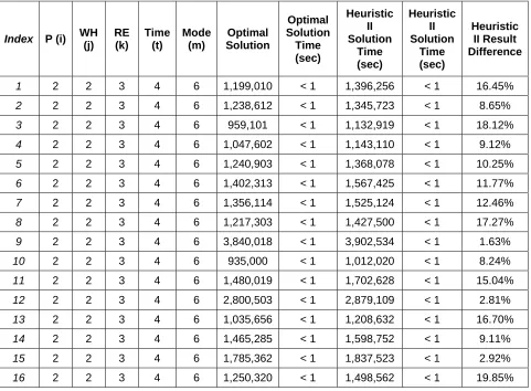
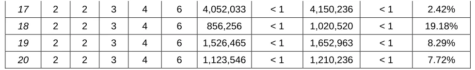
4.5 Heuristic Solution II Result

For consistency and later result comparison, we still use the same data sets to run the

Heuristic Solution II for all “Large”, “Medium” and “Small” size.

We run 20 “Small” data sets first. There is no meaningful time difference between the

optimal solution running and heuristic solution running since the running time for both two is

less than 1 second. The results are shown as below in TABLE 4.4. We can see that the

heuristic result is about 3% ~ 20% worse than the optimal result, which is considered as a

significant difference.

Table 4.4 Result Comparisons between Optimal and Heuristic II for Small Data Sets

Index P (i) WH

(j) RE (k) Time (t) Mode (m) Optimal Solution Optimal Solution Time (sec) Heuristic II Solution Time (sec) Heuristic II Solution Time (sec) Heuristic II Result Difference

1 2 2 3 4 6 1,199,010 < 1 1,396,256 < 1 16.45%

2 2 2 3 4 6 1,238,612 < 1 1,345,723 < 1 8.65%

3 2 2 3 4 6 959,101 < 1 1,132,919 < 1 18.12%

4 2 2 3 4 6 1,047,602 < 1 1,143,110 < 1 9.12%

5 2 2 3 4 6 1,240,903 < 1 1,368,078 < 1 10.25%

6 2 2 3 4 6 1,402,313 < 1 1,567,425 < 1 11.77%

7 2 2 3 4 6 1,356,114 < 1 1,525,124 < 1 12.46%

8 2 2 3 4 6 1,217,303 < 1 1,427,500 < 1 17.27%

9 2 2 3 4 6 3,840,018 < 1 3,902,534 < 1 1.63%

10 2 2 3 4 6 935,000 < 1 1,012,020 < 1 8.24%

11 2 2 3 4 6 1,480,019 < 1 1,702,628 < 1 15.04%

12 2 2 3 4 6 2,800,503 < 1 2,879,109 < 1 2.81%

13 2 2 3 4 6 1,035,656 < 1 1,208,632 < 1 16.70%

14 2 2 3 4 6 1,465,285 < 1 1,598,752 < 1 9.11%

15 2 2 3 4 6 1,785,362 < 1 1,837,523 < 1 2.92%

17 2 2 3 4 6 4,052,033 < 1 4,150,236 < 1 2.42%

18 2 2 3 4 6 856,256 < 1 1,020,520 < 1 19.18%

19 2 2 3 4 6 1,526,465 < 1 1,652,963 < 1 8.29%

20 2 2 3 4 6 1,123,546 < 1 1,210,236 < 1 7.72%

We then run 20 “Medium” data sets. The results are shown as below in TABLE 4.5.

We can see that the heuristic result is about 0.0% ~ 2% worse than the optimal result, which is

much better than the small data sets. In the meanwhile, the running time for the heuristic

solution is sometimes shorter than that of the optimal solution while sometimes longer than

that of optimal solution. The time difference percentage varies a lot from -90% ~ 170%.

Table 4.5 Result Comparisons between Optimal and Heuristic II for Medium Data Sets

Index P

(i) WH (j) RE (k) Time (t) Mode (m) Optimal Solution Optimal Solution Time (sec) Heuristic II Solution Heuristic II Solution Time (sec) Heuristic II Result Difference Heuristic II Time Difference

1 3 4 10 20 12 995,031 5 995,031 10 0.00% 100.00%

2 3 4 10 20 12 1,391,865 16 1,391,864 11 0.00% -31.25%

3 3 4 10 20 12 662,116 7 662,116 8 0.00% 14.29%

4 3 4 10 20 12 3,253,647 100 3,276,895 40 0.71% -60.00%

5 3 4 10 20 12 3,238,801 37 3,250,240 64 0.35% 72.97%

6 3 4 10 20 12 3,465,622 134 3,492,626 15 0.78% -88.81%

7 3 4 10 20 12 2,983,951 102 3,007,255 57 0.78% -44.12%

8 3 4 10 20 12 1,156,357 6 1,156,357 16 0.00% 166.67%

9 3 4 10 20 12 5,892,871 100 5,892,871 56 0.00% -44.00%

10 3 4 10 20 12 5,178,963 67 5,178,963 34 0.00% -49.25%

11 3 4 10 20 12 3,827,174 85 3,856,024 30 0.75% -64.71%

12 3 4 10 20 12 1,352,602 12 1,360,523 12 0.59% 0.00%

13 3 4 10 20 12 5,623,566 80 5,723,695 30 1.78% -62.50%

15 3 4 10 20 12 3,652,525 80 3,679,526 40 0.74% -50.00%

16 3 4 10 20 12 2,235,698 36 2,275,211 25 1.77% -30.56%

17 3 4 10 20 12 4,563,298 156 4,589,635 60 0.58% -61.54%

18 3 4 10 20 12 2,350,256 25 2,350,256 25 0.00% 0.00%

19 3 4 10 20 12 1,658,635 25 1,661,956 40 0.20% 60.00%

20 3 4 10 20 12 1,856,932 35 1,880,563 30 1.27% -14.29%

Finally, we run 20 “Large” data sets, with which Heuristic Solution I doesn’t work out

very well. The results are shown as below in TABLE 4.6. We can see that the heuristic result

is about 0.2% ~ 0.9% worse than the optimal result which is much better than the small data

sets. The best thing is the running time for Heuristic Solution II is much shorter than that of

the optimal solution and heuristic solution I. The time difference percentage between optimal

solution and heuristic solution II varies from -96% ~ -99%.

Table 4.6 Result Comparisons between Optimal and Heuristic II for Large Data Sets

P (i) WH (j) RE (k) Time (t) Mode (m) Optimal Solution Optimal Solution Time (hr) Heuristic II Solution Heuristic II Solution Time (hr) Heuristic II Result Difference Heuristic II Time Difference

1 4 10 30 50 12 26,956,995 19.5 27,005,708 0.25 0.18% -98.72%

2 4 10 30 50 12 26,978,296 19 27,033,882 0.3 0.21% -98.42%

3 4 10 30 50 12 33,802,810 10.2 33,933,464 0.3 0.39% -97.06%

4 4 10 30 50 12 57,143,098 22 57,303,828 0.35 0.28% -98.41%

5 4 10 30 50 12 50,854,257 9.6 51,042,089 0.3 0.37% -96.88%

6 4 10 30 50 12 46,251,260 9.8 46,505,826 0.3 0.55% -96.94%

7 4 10 30 50 12 44,158,897 12.1 44,546,182 0.25 0.88% -97.93%

8 4 10 30 50 12 44,182,192 10.9 44,421,371 0.3 0.54% -97.25%

9 4 10 30 50 12 38,596,650 8.6 38,900,685 0.2 0.79% -97.67%

10 4 10 30 50 12 63,102,530 9.3 63,678,530 0.3 0.91% -96.77%

12 4 10 30 50 12 25,985,420 15 26,102,343 0.25 0.45% -98.33%

13 4 10 30 50 12 48,962,500 11 49,056,230 0.25 0.19% -97.73%

14 4 10 30 50 12 35,625,260 10.2 35,686,996 0.25 0.17% -97.55%

15 4 10 30 50 12 37,569,202 9.6 37,769,658 0.25 0.53% -97.40%

16 4 10 30 50 12 40,258,654 18.2 40,410,326 0.3 0.38% -98.35%

17 4 10 30 50 12 26,532,586 12.9 26,586,028 0.2 0.20% -98.45%

18 4 10 30 50 12 58,623,886 13.5 58,812,005 0.3 0.32% -97.78%

19 4 10 30 50 12 46,102,966 16 46,389,665 0.25 0.62% -98.44%

20 4 10 30 50 12 19,588,230 11.2 19,754,622 0.25 0.85% -97.77%

4.6 Heuristic Solution II vs. Optimal Solution and Heuristic Solution I

Optimal Solution Exponential Distribution

Heuristic Solution II Polynomial Distribution

Heuristic Solution I Polynomial Distribution Computation

Time

Data Size

Figure 4.4: Data Size vs. Computation Time

(Optimal Solution & Heuristic Solution I & Heuristic Solution II)

As Figure 4.4 shown above, when we run Optimal Solution, the running time

exponentially increases with expanding of data size. In contrast, it increases following the

polynomial distribution when we run Heuristic Solution.

From the Heuristic Solution II curve, it is clear that its computation time for Large Data

indicates that Heuristic Solution II saves 96% ~ 99% amount of time comparing to Optimal

5

Result Analysis

5.1 Paired T-test

To compare the optimal results and heuristic result, we conduct the Paired T-tests with

Minitab.

Paired T-Test and CI: SMALL DATA SIZE - Optimal, SMALL DATA SIZE - Heuristic I

Paired T for SMALL DATA SIZE - Optimal - SMALL DATA SIZE - Heuristic I

N Mean StDev SE Mean

SMALL DATA SIZE - Optimal 20 1590571 905721 202525

SMALL DATA SIZE - Heuristic I 20 1643522 900727 201409

Difference 20 -52950.7 22691.6 5074.0

95% CI for mean difference: (-63570.6, -42330.7)

T-Test of mean difference = 0 (vs not = 0): T-Value = -10.44 P-Value = 0.000

Paired T-Test and CI: SMALL DATA SIZE - Optimal, SMALL DATA SIZE - Heuristic II

Paired T for SMALL DATA SIZE - Optimal - SMALL DATA SIZE - Heuristic II

N Mean StDev SE Mean

SMALL DATA SIZE - Optimal 20 1590571 905721 202525

SMALL DATA SIZE - Heuristic II 20 1728993 882540 197342

95% CI for mean difference: (-164827, -112016)

T-Test of mean difference = 0 (vs not = 0): T-Value = -10.97 P-Value = 0.000

Paired T-Test and CI: SMALL DATA SIZE - Heuristic I, SMALL DATA SIZE - Heuristic II

Paired T for SMALL DATA SIZE - Heuristic I - SMALL DATA SIZE - Heuristic II

N Mean StDev SE Mean

SMALL DATA SIZE - Heuristic I 20 1643522 900727 201409

SMALL DATA SIZE - Heuristic II 20 1728993 882540 197342

Difference 20 -85470.8 44762.0 10009.1

95% CI for mean difference: (-106420.1, -64521.5)

T-Test of mean difference = 0 (vs not = 0): T-Value = -8.54 P-Value = 0.000

Paired T-Test and CI: MED DATA SIZE - Optimal, MED DATA SIZE - Heuristic I

Paired T for MED DATA SIZE - Optimal - MED DATA SIZE - Heuristic I

N Mean StDev SE Mean

MED DATA SIZE - Optimal 20 2930290 1558717 348540

MED DATA SIZE - Heuristic I 20 2942258 1565987 350165

Difference 20 -11967.7 18371.2 4107.9

95% CI for mean difference: (-20565.7, -3369.7)

Paired T-Test and CI: MED DATA SIZE - Optimal, MED DATA SIZE - Heuristic II

Paired T for MED DATA SIZE - Optimal - MED DATA SIZE - Heuristic II

N Mean StDev SE Mean

MED DATA SIZE - Optimal 20 2930290 1558717 348540

MED DATA SIZE - Heuristic II 20 2950408 1570210 351110

Difference 20 -20117.7 25134.1 5620.2

95% CI for mean difference: (-31880.8, -8354.6)

T-Test of mean difference = 0 (vs not = 0): T-Value = -3.58 P-Value = 0.002

Paired T-Test and CI: MED DATA SIZE - Heuristic I, MED DATA SIZE - Heuristic II

Paired T for MED DATA SIZE - Heuristic I - MED DATA SIZE - Heuristic II

N Mean StDev SE Mean

MED DATA SIZE - Heuristic I 20 2942258 1565987 350165

MED DATA SIZE - Heuristic II 20 2950408 1570210 351110

Difference 20 -8150.00 9614.90 2149.96

95% CI for mean difference: (-12649.91, -3650.09)

T-Test of mean difference = 0 (vs not = 0): T-Value = -3.79 P-Value = 0.001

Paired T for LARGE DATA SIZE - Optimal - LARGE DATA SIZE - Heuristic II

N Mean StDev SE Mean

LARGE DATA SIZE - Optimal 20 39831792 12348167 2761134

LARGE DATA SIZE - Heuristic II 20 40021235 12425888 2778513

Difference 20 -189443 128825 28806

95% CI for mean difference: (-249735, -129151)

T-Test of mean difference = 0 (vs not = 0): T-Value = -6.58 P-Value = 0.000

The Minitab results show a very low P-value which indicates that there is significant

difference between Optimal Solution and Heuristic Solution.

5.2 One – Sample T- Test Analysis

Paired T-test shows that there is significant difference between Optimal Solution and

Heuristic Solution, the data shows a very small difference though. We then conduct

One-Sample T-Test on percentage difference between optimal and heuristic for both result and

Table 5.1 Percentage Difference between Optimal Solution and Heuristic Solution

Small

Data Size Medium Data Size Large Data Size

Index Heuristic I Result Difference Heuristic I Result Difference Heuristic I Time Difference Heuristic II Result Difference Heuristic II Time Difference Heuristic II Result Difference Heuristic II Time Difference

1 5.91% 0.00% 1100.00% 0.00% 100.00% 0.18% -98.72% 2 2.59% 0.00% 5525.00% 0.00% -31.25% 0.21% -98.42% 3 6.56% 0.05% 1614.29% 0.00% 14.29% 0.39% -97.06% 4 2.23% 0.37% 1700.00% 0.71% -60.00% 0.28% -98.41% 5 7.33% 0.24% 3143.24% 0.35% 72.97% 0.37% -96.88% 6 1.59% 0.14% 795.52% 0.78% -88.81% 0.55% -96.94% 7 4.94% 0.22% 1076.47% 0.78% -44.12% 0.88% -97.93% 8 4.02% 0.00% 1566.67% 0.00% 166.67% 0.54% -97.25% 9 1.16% 0.00% 1100.00% 0.00% -44.00% 0.79% -97.67% 10 3.19% 0.00% 1392.54% 0.00% -49.25% 0.91% -96.77% 11 4.89% 0.11% 1311.76% 0.75% -64.71% 0.49% -97.78% 12 0.53% 0.29% 900.00% 0.59% 0.00% 0.45% -98.33% 13 6.50% 1.28% 1400.00% 1.78% -62.50% 0.19% -97.73% 14 4.17% 1.43% 1823.08% 1.86% -51.92% 0.17% -97.55% 15 1.86% 0.62% 1400.00% 0.74% -50.00% 0.53% -97.40% 16 7.60% 0.89% 2400.00% 1.77% -30.56% 0.38% -98.35% 17 1.25% 0.29% 1053.85% 0.58% -61.54% 0.20% -98.45% 18 8.08% 0.00% 3900.00% 0.00% 0.00% 0.32% -97.78% 19 4.20% 0.13% 3500.00% 0.20% 60.00% 0.62% -98.44% 20 3.45% 1.22% 2757.14% 1.27% -14.29% 0.85% -97.77%

For Small Data Size, the mean of the result difference is 4.1%. As we noted before,

there is no noticeable time difference between the optimal solution running and heuristic

solution running since the running time for both is less than 1 second. Needless to say, there is

no significant advantage by implementing Heuristic Solution on Small Data Size Model.

Variable N Mean StDev SE Mean 95% CI

Heuristic I Resu 20 0.041019 0.023263 0.005202 (0.030132, 0.051906)

Heuristic I Result Diff-Small

0.09 0.08

0.07 0.06

0.05 0.04

0.03 0.02

0.01 0.00

_ X

Boxplot of Heuristic I Result Diff-Small

(with 95% t-confidence interval for the mean)

For Medium Data Size, we compare the results for both Heuristic Solution I and

Heuristic Solution II. As for Heuristic Solution I, the Mean value of the result difference is

0.36%, which can be considered a very small sacrifice from the optimal solution. However,

the trade off of Heuristic I is unacceptable. The Mean value of the running time is increased

by 1972.98%.

Variable N Mean StDev SE Mean 95% CI

Heuristic I Resu 20 0.003648 0.004681 0.001047 (0.001457, 0.005839)

He u r is t ic I R e s u lt Diff- M e d iu m

0.0 16 0 .01 4

0.0 12 0.0 10

0 .00 8 0.0 06

0 .00 4 0.0 02

0 .00 0

_ X

B o x plo t o f H e ur is tic I R e s ult D iff- M e dium (w ith 95 % t-co nfide nce inte r va l fo r the m e a n)

One-Sample T: Heuristic I Time Diff-Medium

Variable N Mean StDev SE Mean 95% CI Heuristic I Time 20 19.7298 12.2175 2.7319 (14.0118, 25.4477)

He urist ic I Time Diff-Me dium

60 50

40 30

20 10

_ X

Boxplot of Heuristic I Time Diff-Medium

We then look at Heuristic Solution II for Medium Data Size. The Mean value of the

result difference is 0.61%, which can be considered minor. The Mean value of the running

time difference is -11.95%, which means that the running time is decreased by applying

Heuristics Solution II. Standard Deviation and 95% Confidence Interval are calculated for

running time difference. Its Standard Deviation is 65.3%, and its 95% confidence interval

ranges from -42.5% to 18.6% which is not stable and too wide to be predicted.

One-Sample T: Heuristic II Result Diff-Medium

Variable N Mean StDev SE Mean 95% CI

Heuristic II Res 20 0.006081 0.006346 0.001419 (0.003111, 0.009051)

Heuristic II Result Diff-Medium

0.020 0.015

0.010 0.005

0.000

_ X

Boxplot of Heuristic II Result Diff-Medium

(with 95% t-confidence interval for the mean)

One-Sample T: Heuristic II Time Diff-Medium

Variable N Mean StDev SE Mean 95% CI

Heuristic II Time Diff-Medium

2.0 1.5

1.0 0.5

0.0 -0.5

-1.0

_ X

Boxplot of Heuristic II Time Diff-Medium

(with 95% t-confidence interval for the mean)

For Large Data Size, we only conduct Heuristic Solution II since Heuristic Solution I

takes way too long time to run through the end. The Mean value of the result difference is

0.47%, which can be considered minor trade off from the optimal solution. Moreover, the

Heuristic II substantially reduces the running time. The Mean value of the running time

decreasing is 97.8%. Its 95% confidence interval ranges from 98.1% to 97.5%, which is

considered reliable.

One-Sample T: Heuristic II Result Diff-Large

Variable N Mean StDev SE Mean 95% CI

Heuristic II Result Diff-Big

0.010 0.009

0.008 0.007

0.006 0.005

0.004 0.003

0.002 0.001

_ X

Boxplot of Heuristic II Result Diff-Big

(with 95% t-confidence interval for the mean)

One-Sample T: Heuristic II Time Diff-Large

Variable N Mean StDev SE Mean 95% CI

Heuristic II Time Diff-Big

-0.970 -0.975

-0.980 -0.985

-0.990

_ X

Boxplot of Heuristic II Time Diff-Big

6

Conclusion & Future Research

The supply chain model presented in this study consists of 3 layers of variables –

Plant, Warehouse and Retailer. We tested the Mathematical Model with Small Data Size,

Medium Data Size and Large Data Size, and apply Heuristic Solution I and Heuristic Solution

II on them respectively. Upon performing further statistic analysis on the test results, we draw

our conclusions as summarized in the following table:

Table 6.1 Summary and Conclusion

Optimal Solution Heuristic Solution I Heuristic Solution II

Result Time Result Time Result Time

Recommendations

Small

Data - < 1 sec

4.1%

worse < 1 sec

10.9%

worse < 1 sec Run Optimal

Medium

Data -

About 1 min 0.36% worse 20 min (1973% longer) 0.61% worse 40 sec (12% shorter) Run Optimal Large

Data -

About 13

hrs - >72 hrs

0.47% worse 15 min (98% shorter) Run Heuristic Solution II

i) Small Data Size -

(2 Plants, 2 Warehouses, 3 Retailers, 4 Time Periods and 6 Transportation

The run time for Optimal Solution is less than 1 second. When Heuristics

Solution is applied to data sets of this size, the deviation from optimal result is over

4.1% and 10.9% for Heuristic Solution I and II respectively. Hence the Optimal

Solution best fits data sets of this size.

ii) Medium Data Size -

(3 Plants, 4 Warehouses, 10 Retailers, 20 Time Periods and 12 Transportation

Modes)

The run time of Optimal Solution is about 1 minute. In the case of Heuristic

Solution I, the running time is about 15 minutes, much longer than the optimal

solution time. In the case of Heuristic Solution II, the average running time is about 30

seconds, and the heuristic result impairs by 0.61% on average. However, because the

standard deviation for both running time decreasing and result value increasing is

significant, Heuristic Solution II is less likely yield reliable results for Medium Data

Size either. Optimal Solution is the best choice for Medium data size as well.

iii) Large Data Size -

(4 Plants, 10 Warehouses, 30 Retailers, 50 Time Periods and 12 Transportation

Modes)

The optimal solution running time is about 13 hours, which is excessive. With

Heuristic Solution I, the running time is even much longer than the optimal solution

running time. Heuristic Solution I will clearly be rejected. In contrast, the running time

running time is about 15 minutes, and the heuristic result is impaired by 0.47%

averagely. Moreover, the standard deviation for both running time decreasing and

result value increasing is insignificant. Heuristic Solution II is therefore recommended

for large size of data.

Our proposed deterministic model clearly reflects a strategy of total supply chain

management. The result analysis demonstrates that our stepwise heuristic optimization with

CPLEX/OPL coding is novel and powerful in solving supply chain models of fairly large data

sets.

The research discussed in this thesis is the foundation for many potential areas of

future work,

i) More Layers –

The mathematical model in this paper consists of 3 layers, which are Plant,

Warehouse and Retailer. There could be more components in a real-world supply

chain, e.g. raw material supplier, sub-contract manufacturer, distribution center, etc.

These layers could be taken into account to make the model more realistic.

ii) More products –

There is only one product considered in this paper, which is not typical in real

manufacturing world. Realistic supply chains have multiple end products with shared

components, facilities and capacities. Multi-products could be investigated.

In this paper, only 1 cost coefficient is applied at each location and there is no

setup cost considered for all the operations. Operation cost at each location could be

broke down into more detailed level, like labor cost, material cost, etc. Setup cost for

each plant/warehouse/retailer could be considered as well.

iv) Safety inventory at each location –

In our model, there is no inventory stored at all plants, whatever produced are

shipped out. While, manufacturers always keep some safety stock to satisfy customer

needs better. Different safety inventory level could be applied to make the model more

practical.

v) User Interface –

We build all the model, data and script in CPLEX/OPL. It is not convenient to

be applied by any end-user. The customer interface could be build to make this model

7

Bibliography

Chung-Piaw, T. and Shu, Jia Warehouse-Retailer Network Design Problem Operations

Research, v 52, n 3, May/June, 2004, pp 396-408+497

Cohen, M.A. and Lee, H.L. Strategic Analysis of Integrated Production-Distribution Systems:

Models and Methods, Operations Research, v 36, n 2, Mar-Apr, 1988, pp 216-228

Cohen, M.A. and Lee, H.L. Resource Deployment Analysis of Global Manufacturing and

Distribution Networks, Journal of Manufacturing and Operations Management, v 2, n 2,

Summer 1989, pp 81-104

Geoffrion, A.M. and Graves, G.W. Multicommodity Distribution System Design by Benders

Decomposition, Management Science, v 20, n 5, Jan, 1974, pp 822-844.

Iida, T. A non-stationary periodic review production-inventory model with uncertain

production capacity and uncertain demand, European Journal of Operational Research, v

140, n 3, Aug 1, 2002, pp 670-683

Jack, G.A.J., Vorst, V.D., Beulens, A.J.M. and Beek, P.V. Modelling and Simulating

Multi-echelon Food Systems, European Journal of Operational Research, v 122, n 2, Apr, 2000, pp

Lee, H.L. and Billington, C. The Evolution of Supply Chain Management Models and

Practice at Hewlett-Packard, Interfaces, v 25, n 5, Sept.-Oct. 1995, pp 42-63

Lee, Y.H. and Kim, S.H. Production-Distribution Planning in Supply Chain Using a Hybrid

Approach, Production Planning and Control, v 13, n 1, January/February, 2002, p 35-46

Lee, Y.H. and Kim, S.H. Production-Distribution Planning in Supply Chain Considering

Capacity Constraints, Computers and Industrial Engineering, v 43, n 1-2, Jul, 2002, pp

169-190

Matta, Renato de and Miller, T. Production and inter-facility transportation scheduling for a

process industry, European Journal of Operational Research, v 158, n 1, Oct 1, 2004, pp

72-88

Simichi-Levi, D., Kaminsky, P. and Simichi-Levi, E. Designing and Managing the Supply

Chain: Concepts, Strategies, and Case Studies, 2001, Irwin/McGraw-Hill

Yang, Po-Chung and Wee, Hui-Ming Economic Ordering Policy of Deteriorated Item for

Vendor and Buyer: An integrated approach, Production Planning and Control, v 11, n 5,

2000, pp 474-480

Yang, Po-Chung and Wee, Hui-Ming The Optimal and Heuristic Solutions of A Distribution

Barbarosoglu, Gulay An Integrated Supplier-Buyer Model for Improving Supply Chain

Coordination,