Algorithms
.
White Rose Research Online URL for this paper:
http://eprints.whiterose.ac.uk/108877/
Version: Accepted Version
Article:
Bonilla Licea, D, McLernon, D and Ghogho, M orcid.org/0000-0002-0055-7867 (2017)
Mobile Robot Path Planners with Memory for Mobility Diversity Algorithms. IEEE
Transactions on Robotics, 33 (2). pp. 419-431. ISSN 1552-3098
https://doi.org/10.1109/TRO.2016.2636848
© 2017 IEEE. This is an author produced version of a paper published in IEEE
Transactions on Robotics. Personal use of this material is permitted. Permission from
IEEE must be obtained for all other uses, in any current or future media, including
reprinting/republishing this material for advertising or promotional purposes, creating new
collective works, for resale or redistribution to servers or lists, or reuse of any copyrighted
component of this work in other works. Uploaded in accordance with the publisher's
self-archiving policy.
[email protected] https://eprints.whiterose.ac.uk/ Reuse
Unless indicated otherwise, fulltext items are protected by copyright with all rights reserved. The copyright exception in section 29 of the Copyright, Designs and Patents Act 1988 allows the making of a single copy solely for the purpose of non-commercial research or private study within the limits of fair dealing. The publisher or other rights-holder may allow further reproduction and re-use of this version - refer to the White Rose Research Online record for this item. Where records identify the publisher as the copyright holder, users can verify any specific terms of use on the publisher’s website.
Takedown
If you consider content in White Rose Research Online to be in breach of UK law, please notify us by
Mobile Robot Path Planners with Memory for
Mobility Diversity Algorithms
Daniel Bonilla Licea, Des McLernon, Mounir Ghogho
Abstract—Mobile robots using wireless communications often experience small-scale fading and due to this the wireless channel gain can be low. If the channel gain is poor (due to fading) the robot can move (a small distance) to another location in order to improve the channel gain and so compensate fading. Techniques using this principle are called mobility diversity algorithms (MDAs). MDAs intelligently explore a number of points in order to find a location with high channel gain while using little mechanical energy during the exploration. Up until now the location of these points has been predetermined. In this paper, we show how we can adapt their positions by using channel predictors. Our results show that MDAs, which adapt the location of those points, can in fact outperform (in terms of the channel gain obtained and mechanical energy used) the MDAs that use predetermined locations for those points. These result will significantly improve the performance of the MDAs and consequently allow MRs to mitigate poor wireless channel conditions in an energy efficient manner.
Index Terms—Autonomous Agents, Robotics Communications, Fading
I. INTRODUCTION
A. Motivation and Overview
W
IRELESS communications is nowadays an important aspect of mobile robotics and we find in this research area various problems being studied. In [6] the authors de-sign a control law for a drone to follow a ground robot while maintaining a minimum data rate in an optical wireless communications link; in [9] and [10] the authors consider a team of autonomous robots in which a leader must perform a certain task while the other robots must optimize their position in order to maintain a certain quality in the wire-less end-to-end communications link from the leader to an access point; in [8] and [11] the authors consider a similar problem in which which an autonomous robotic network must attain a desired target position while maintaining a certain communications quality; then in [7] the authors maximize the coverage area of a mobile sensor network while ensuring wireless communications between its members; in [12] the authors consider a cooperative mobile sensor network and then design control laws so that at each iteration the sensor nodes gather a maximum amount of information. Another important problem in robotics communications (which is not treated inDaniel Bonilla Licea is with the University of Leeds, UK, e-mail:[email protected]. The author acknowledges the funding of CONACYT, Mexico.
Des McLernon is with the University of Leeds, UK, e-mail: [email protected].
Mounir Ghogho is with the University of Leeds, UK and the International University of Rabat, Morocco, e-mail: [email protected].
[6]-[12]) is the compensation of small-scale fading in wireless channels using the mobility of the robot [24]-[?].
Small-scale fading (also called multi-path fading) occurs in RF wireless links when, due to reflection and refraction, multiple copies of the transmitted signal arrive simultaneously at the receiver’s antenna each one with different phase and then create either constructive or destructive interference. In consequence the strength of the received signal is a random variable which varies significantly over very small distances (on the order of one wavelength). If small-scale fading is not compensated then it can degrade and even impede wireless communications. Therefore the need of compensating the small-scale fading. This can be done using classical diversity multi-antenna techniques [35] which have originally been devised in the communications community for transceivers that cannot control their location (e.g., mobile phones) or alternatively by using antennas with high directionality as in [13] and [14]. Nevertheless, it has been shown that we can by controlling the position of the robot we can compensate small-scale fading [17]-[?]. This class of techniques have been referred to as mobility diversity algorithms [21], spatial diversity [15], jittery movements [19] among other names. In this article we will refer to this class of techniques as mobility diversity algorithms (MDAs).
To the author’s knowledge the first work in which mobility was controlled in order to compensate small-scale fading is [15]. In that paper the authors consider an RF wireless link ex-periencing small-scale fading and they showed experimentally that: (i) when the channel gain is bad due to the small-scale fading individuals can move in the surroundings to alter the physical configuration of the scatterers and therefore to alter the small-scale fading in order to try to obtain high channel gains in the wireless channel; (ii) it is possible to move the transmitter very small distances in order to find a position in which the channel gain is high. In other words the authors showed that we can take advantage of the small-scale fading by either altering the physical configuration of the surroundings or by altering the position of the transmitter. In that paper, the authors provided mobility to a transmitter node by placing it on a motorized turntable and so the transmitter moves in a circular path. The channel is then measured at various points along that circular path and the node stops at a position when the channel gain is high. This technique was used by the same authors in [16] to compensate small-scale fading in a wireless sensor network.
must be added to the nodes which can result an expensive solution. Nevertheless note that in the context of robotics communications the transceivers are mounted on the mobile robots and thus they already posses this capacity. The main problem to be solved in MDAs is how to determine the location of the points to be explored by the robot. This is a relatively new problem and the amount of literature dealing with this it is scarce. Now, we present the most important works that have considered this problem.
In [17] the authors consider the problem of moving the robot to compensate small-scale fading but without deviating too much from its initial position. The authors suggest to make the robot explore a finite number of points and then make it return to the point that exhibits the best channel gain. Regarding the physical configurations of the points explored by the robot the authors propose two configurations: (i) points arranged in a circular path; (ii) points arranged in an hexagonal lattice contained into a circle. The size of both configurations are calculated in order to obtain independent wireless channels.
Then in [18] the authors corroborated experimentally that indeed we can improve the channel gain of wireless channels experiencing small-scale fading by controlling the position of the robot. In that paper the authors propose to move the robot in a straight, circular, spiral-like and random paths while taking samples of the wireless channel in order to find a position with high channel gain.
Other physical configurations for the points that the robot explore during an MDA execution are proposed. For example, in [19] the authors propose to compensate small-scale fading by exploringN points randomly distributed in a small circle centered around the robot’s initial position and then making the robot go to the point with highest channel gain. In that paper the number of points and the size of the circle are design parameters arbitrarily determined. In [20] the authors consider a robotic wireless network and they compensate small-scale fading using and MDA. In their experiments they made each robot to explore five positions arranged in a circular uniform array with central element and radiusλ/2and then it chooses the best position according to a network metric. That configuration for the explored points provides five statistically independent wireless channels. Finally in [21] we presented a technique to calculate the optimum position of the points in order to maximize the expected value of the channel channel gain obtained while minimizing the amount of mechanical energy used in motion during the MDA execution.
In [15]-[21] the authors propose different configurations for the points explored by the robot in order to compensate for the small-scale fading but another variant to this problem is the one considered in [23] and [24]-[27] where the authors consider that the mobile robot must follow a predefined path while communicating with a base station through an RF wireless channel experiencing small-scale fading. In this case, as opposed to [15]-[21], in order to compensate the small-scale fading the authors do not focus on determining the location of the points where the robot transmits but rather on determining its velocity profile. The solution in those articles is roughly based on the idea of following the predetermined path but spending more time at points (in the predefined path) with high
channel gain (due to constructive interference generated by the small-scale fading) and less time at points (in the predefined path) with poor channel gain (due to destructive interference generated by the small-scale fading). Note that this approach works due to the fact that in the presence of small-scale fading channel gain varies significantly over small distances.
In this current article we will focus on the variant of the problem considered in [15]-[21]. Thus the main problem considered in this article is to optimally determine the location of the points explored by the robot, in its close vicinity, in order to compensate for the small-scale fading. Note that in [15]-[21] the location of the explored points is predetermined. In other words, the location of the points is fixed at the beginning of the MDA execution. We will refer to this class of configurations for the explored points as predetermined geometries.
An alternative to predetermined geometries are the adaptive geometries. In this case the location of the points explored by the robot are determined online according to the measure-ments and locations of the previously explored points. This is achieved using path planners with memory. In [22] we proposed path planners with memory order one and two for the MDAs and we observed that, given the numberN of explored points, the performance of the MDA in terms of channel gain obtained and average distance travelled by the robot during the MDA execution was better when we used the path planner with memory order two than when we used the path planner with memory order one. This suggests that, in the context of MDAs, the higher the memory order of the path planner the better the performance of the MDA can be. Furthermore, since predetermined geometries can be interpreted as the result of memoryless path planners this would also suggest that MDAs using path planners with memory can outperform MDAs with predetermined geometries. In order to confirm this hypothesis and obtain better performance in the MDAs we need to develop path planners with higher memory order for the MDAs.
B. Contribution and Organization
In this paper we will develop path planners with arbitrary memory order for MDAs. We provide a solid theoretical foundation for these path planners and finally we will show that MDAs that use path planners with memory can outperform those that use predetermined geometries. Since the MDAs considered in [15]-[21] use predetermined geometries this last result imply that MDAs using the path planners with memory presented in this paper outperform the MDAs presented in all those articles. In more detail, the main contributions of this article are:
1) Showing the advantages of executing MDAs using path planners with memory respect to executing them using predetermined geometries. As mentioned above this result implies that the MDAs using the path planners with memory proposed in this paper can outperform the MDAs presented in [15]-[21].
points are explored. This analysis will allow us to gain insight into the general properties of the wireless channels obtained by using path planners with memory and then observe how these properties differ respect to the case when predetermined geometries are used. 3) General solutions for the path planner with an arbitrary
memory order. In [22] we proposed a path planner with memory order one and two. In this paper we first derive in a more rigourous way path planners with memory order one and two and then using that theory we develop path planners with arbitrary memory order. This is motivated by the fact that according to the results in [22] it would seem that path planners with higher memory order can perform better and thus by developing path planners with higher memory order we can validate this hypothesis.
4) It is widely known in the communications literature that correlation degrades the performance of all the classical diversity techniques ( see chapter 9 of [35]). In other words in all classical diversity techniques their performance is maximized when all the channels are independent. But in this article we show that by con-trolling in smart way channel correlation (with help of the path planners with memory) we can improve the performance of MDAs even respect to the case when all the wireless channels are independent. Thus showing that, unlike other classical diversity techniques, MDA is a unique type of diversity which can benefit from channel correlation.
In section II we state the mathematical model for the MR and the model for the wireless channel. We also describe in more detail the mobility diversity algorithm and we show how the path planner forms part of it. Then in section III we derive a path planner with memory one and in section IV we provide a detailed analysis of it for the special case when only two points are considered; in section V we derive path planners with memory order two and then in section VI we show how to derive path planners with an arbitrary memory order. Simulations of the path planners are given in section VII and finally we provide conclusions in section VIII.
II. SYSTEMMODEL
A. Wireless Channel Model
We consider that the MR is trying to communicate with a stationary node (e.g. another MR, a sensor node or a base station). We assume that there is no line of sight between the MR and the stationary node, the signal transmitted by the stationary node to the MR is narrowband, the environment is stationary (i.e., it does not change with time during the execution of the MDA) and there is a large number of scatterers. Consequently, the wireless channel between the MR and the stationary node is time-invariant (over the duration that the MR is stationary) and experiences Rayleigh flat-fading. Thus, the signal received by the MR when located at position
q at timet. is:
y(t,q) =s(p(t))h(q)x(t) +n(t) (1)
where x(t) is the narrowband signal transmitted by the stationary node, n(t) ∼ CN(0, σ2
n) is1 the additive white
Gaussian noise. Thens(p(t))andh(p(t))∼ CN(0,1)are the shadowing (also known as large-scale fading) [34] and small scale fading terms respectively (both depending on the MR’s position,p(t)). We will assume Jakes’ model [30] for the small scale fading and so h(q) can be considered a bidimensional homogenous and isotropic [31] random and complex scalar field with h(q) ∼ CN(0,1). So the following normalized spatial correlation function holds:
r(p,q) =E[h(p)h∗(q)] =J
0(2πkp−qk2/λ), (2)
whereλis the wavelength used in the RF transmission by the stationary node andp,q∈R2are any two points in the space. For the reader who may not be familiarized with the communications literature we clarify that the wireless channel refers to s(p(t))h(q) and the channel gain refers to its modulus.
B. Mobility Diversity Algorithm
In this article, we consider an omnidirectional MR2. In par-ticular we select a three-wheel omnidirectional mobile robot3 (TOMR) [28]. A TOMR is a MR with three omnidirectional wheels [29], each wheel driven by its own motor. The robot is equipped with an antenna installed on its geometrical center. The TOMR’s position at timetin the global coordinate frame isp(t).
For the MDA we consider the following version of the MDMTA [21], [?] that maximizes the power of the channel gain obtained. By definition the initial position of the MR is the stopping point q1. At time instant tk (with k =
1,2,· · · , N−1) the MR is located at the stopping pointqkand
it estimates the wireless channel at this point. Then, it invokes a path planner to calculate the position of qk+1 and moves
in straight line towards it. This stage is called the searching phase. Once the MR reachesqN thesearching phasefinishes.
Then, it invokes a selection rule to determine the ‘optimum stopping point’qoptas the explored stopping point with largest
channel gain and so moves to qopt. At time instant tN+1 it
reachesqoptand then the MDA terminates. This last stage is
called theselection phase. Once the MDA terminates the MR establishes communication with the stationary node.
The area explored by the MR during the execution of the MDA is small (on the order of a couple of wavelengthsλ) and so we will assumes(p(t))≈s. This means that the shadowing term in (1) will be the same for all the stopping points. This assumption on the shadowing term can be justified by the experimental results in [3].
As opposed to [21], in this paper we will consider that the location of the stopping points is adaptive rather than
1Note thatCN(0, σ2)means a complex normal random variable with zero
mean, varianceσ2and whose real and imaginary parts are independent and
identically distributed.
2An omnidirectional MR is a mobile robot that can move in any direction
at any time.
3Although we restrict our analysis to a TOMR, the technique presented in
predetermined. The general form of the path planner that we will use is:
qk+1=fM(k)
QM(k)(k),HˆM(k)(k), k
(3)
where M(k) is the memory order of the path plan-ner, QM(k)(k) = [qk−M(k)+1, qk−M(k)+2,· · · ,qk]T,
ˆ
HM(k)(k) = [ˆh qk−M(k)+1
, ˆh qk−M(k)+2
· · ·,ˆh(qk)]T,
ˆ
h(qk) is the estimation for h(qk) with estimation error
ˆ
h(qk)−h(qk)∼ CN(0, σ2
e)andfM(k)(·,·,·)is the iterative
path planner function with memory orderM(k)(IPPF-M(k)) to be developed and analyzed throughout this article. Note that the path planner (3) requires an estimate of the small-scale fading term. Nevertheless the channel estimation process estimates the productsh(q). Therefore to implement this path planner the MR needs to have an estimate of s in order to isolate the shadowing term from the estimate of the product
sh(q). The shadowing term s can be estimated prior to the MDA execution with a technique like the one stated in [4] (implemented by this MR or by a robotic network). Hence we will assume in this article that the MR has an estimate of s. In addition, since we assume that s is known and that it is constant for all the stopping points then it has no effect on the the results and analyses presented in this paper. Therefore, in order to simplify the notation, we will ignore it in the rest of the paper.
As mentioned previously, we assume that the MR moves from stopping point to stopping point in a straight line. In addition we assume that this is done using an optimal control law that minimizes the energy needed for motion [32]. So for the TOMR considered in this paper the energy used in moving in straight line fromqk toqk+1 in a timetk+1−tk is given
by [21]:
Em(k, k+ 1) =K(tk+1−tk)kqk+1−qkk22 (4)
whereK(tk+1−tk)is a function oftk+1−tkand its expression
can be obtained by matching (4) with the energy expression in [21]. For simplicity, over the rest of the paper we will restrict
tk+1−tk=T.
During the searching phase, at time instant tk the MR
knows {ˆh(qj)}kj=1 but the IPPF-M(k) has only access to
{ˆh(qj)}kj=k−M(k)+1because it has memory orderM(k)≤k.
Now, we define the followingM(k)×M(k)correlation matrix
C(k, M(k))with entries:
Cmn(k, M(k)) =r(qk−M(k)+m,qk−M(k)+n) (5)
and let˜hM(k)(qk+1)be the IPPF-M(k)’s predictor model for
h(qk+1)at time instanttk. It is not difficult to show that:
˜
hM(k)(qk+1) =
p(k+ 1, M(k) + 1)
P−1(k, M(k)) ˆH
M(k)(k)
gk+1
wheregk+1∼ CN(0,1)andgj andgk are independent ifk6=
j;C(k, M(k)) =P(k, M(k))PT(k, M(k))
withP(k, M(k))
being a lower triangular matrix andp(k+ 1, M(k) + 1)is the last row of the matrix P(k+ 1, M(k) + 1).
For mathematical simplicity we will assume that the esti-mation error is negligible and soˆh(qk) =h(qk). Then, in the
simulation section VII we will observe the effect of this error on the algorithms that have been developed.
III. PATHPLANNERS WITHMEMORYORDERONE
In this section we develop the iterative path planner in (3) with memory order one, i.e., with M(k) = 1. We will refer to this path planner as IPPF-1 and its general form is:
f1(qk, h(qk), k) = d1(h(qk))v(k) +qk, (6)
v(k) = [cos(ψ(k)) sin(ψ(k))]T
(7)
where d1(h(qk)) is a distance function that determines the
distance between thekth and thek+ 1th stopping points (i.e.,
kqk+1−qkk2) andψ(k)is the direction in which the MR has
to move to arrive atqk+1 departing fromqk.
The main objective of an MDA is to obtain high channel gain while using little mechanical energy. So, one way to op-timize the IPPF-1 in (6) is to solve the following optimization problem:
max
d1(h(qk)),ψ(k)
θE[|h(qopt)|]−(1−θ)E
"N
X
k=1
Em(k, k+ 1)
#
s.t.
qk+1=d1(h(qk))v(k) +qk k= 1,2,· · ·, N−1
q1=0,
qN+1=qopt
(8) The optimization target in (8) is a convex combination of the expected value of the channel gain at qopt and the negative
of the average mechanical energy used during the MDA execution. We remind to the reader thatqopt is the optimum
stopping point selected by the selection rule, see section II-B. The design parameterθ∈[0,1]defines the importance of one term over the other. The motivation for this optimization target is that we want a path planner that when used as part of the MDA provides the MR with a high channel gain while using little mechanical energy. So we can see this as an ‘investment problem’, where we want to maximize the profit given by the difference between the income (the optimum channel gain obtained) and the investment (the energy used in motion).
The first two equality restrictions in (8) refer to the fact that the stopping points are calculated using the IPPF-1 and that the first stopping point is at 0. The third equality restriction is added for notational convenience to simplify the expression of the term that represents the mechanical energy used during the whole algorithm execution (i.e., from time instantt1until
tN+1) in the optimisation target in (8).
This optimization target is a functional that depends on the functions d1(h(qk)) and ψ(k) and theoretically it could be
solved using dynamic programming [32]. But, in general there is no an analytical expression for the optimization target in (8)(specifically for the term E[|h(qopt)|]) so in practice we
must evaluate it by Monte Carlo simulations thus making the optimization process computationally expensive. This problem is accentuated by the fact that the optimisation target depends on two functions rather than a single one.
This can be alleviated by first optimisingd1(h(qk))
using the previously optimizedd1(h(qk)). This produces two
optimization problems with smaller search spaces which are simpler and computationally cheaper to solve than directly trying to solve (8).
We can further simplify the optimization of d1(h(qk))
by restricting it to be a specific parameterized function and then optimize its parameters. This is because optimizing a few parameters of a function is computationally cheaper than finding the optimal form of the function itself. To achieve this we first note that forM(k) = 1the predictor (6) can be written as:
˜
h1(qk+1) =gk+1
p
1−r2(q
k,qk+1) +h(qk)r(qk,qk+1),
(9) with power:
Eh|˜h1(qk+1)|2
i
= (1 +rk,k+1(|h(qk)|2−1)). (10)
For notational simplicity, we will use interchangeably
r(qk,qj)andrk,j in the rest of the paper. From (10) and (2)
we observe that if the MR wants to maximize the power of the predicted channel at qk+1 it must move near (far) fromqk to
experience a high (low) correlation factor rk,k+1 if |h(qk)|2
is high (low). Note that the implementation of this idea results in iterative path planner with memory order one in [22]. If we restrict d1(h(qk))to implement this idea then:
d1(h(qk)) =1R+∗(|h(qk)| −η)d+1R−(|h(qk)| −η)D,
(11) where1R+∗(·)is the indicator function andd < D andη are
the parameters to be optimized according to:
max
d,D,ηθE[|h(qopt)|]−(1−θ)E
"N
X
k=1
kqk+1−qkk22
#
s.t.
qk+1=d1(h(qk))v(k) +qk k= 1,2,· · · , N−1,
d1(h(qk)) =1R+∗(|h(qk)| −η)d+1R−(|h(qk)| −η)D,
q1=0, qN+1=qopt, ψ(k) =ψ(1).
(12) This optimization problem is obtained by restricting
d1(h(qk))to take the form in (11) and absorbing the term
K(T)of the mechanical energy term (see (4)) into the multi-plying factor 1−θ. This optimization problem can be solved numerically using simulated annealing. In general there is no an analytical expression for the cost function and so it must be evaluated by simulations but for the particular case ofN = 2
stopping points we are able to derive an analytical expression for the cost function, as shown in subsections IV-B and IV-D. Note that the cost function in (12) depends indirectly on the parameters d,D and η. This is because the cost function depends on the stopping points and these are calculated using those parameters as it can be seen from the first and second equality restrictions in (12).
Now, given d1(h(qk)), the function ψ(k) determines the
distance traveled by the MR during the selection phase4, the distance among the stopping points and so the correlation between their wireless channels and consequently it also
4The distance traveled during the searching phase depends only on d1(h(qk))and not onψ(k).
affects the statistics of h(qopt). So, a poor choice of ψ(k)
can significantly decrease E[h(qopt)|] and/or maximize the
amount of mechanical energy used during theselection phase. Therefore the necessity of optimizingψ(k)is clear. Given the number of stopping points (N) and the optimized function
d1(h(qk))we can optimizeψ(k)by solving the following:
max
ψ θE[|h(qopt)|]−(1−θ)E
kqopt−qNk22
s.t.
qk+1=d∗1(h(qk))v(k) +qk k= 1,2,· · · , N−1,
q1=0,
ψ(k+ 1)−ψ(k) =ψ k= 1,2,· · · , N−2,
(13) whered∗
1(h(qk))is the optimized distance function according
to (12). The first term in the cost function is the expected value of the maximum channel gain obtained by the MR and the second term is the expected value of the distance traveled during the selection phase. This is because, as mentioned previously, only the distance traveled during the selection phaseis affected by ψ(k). In the cost function, the first term will tend to spread out the stopping points to reduce the correlation among all the points and to increaseE[|h(qopt)|]
but the second term will tend to concentrate the stopping points around qN to reduce the distance traveled during the
selection phase. Now, the last equality restriction of (13) reduces the dimension of the search space fromN −2 to1. This is done because there is not an analytical expression for the cost function and so reducing the search space simplifies significantly the optimization process (although it also reduces the performance).
So now that we have shown how to optimized1(h(qk))and
ψ(k) in (6) we have concluded the design of the IPPF-1 in (6). In the next section we will analyze some of the properties of the IPPF-1 presented in this section for the particular case whenN= 2. We will also derive the analytical expression for the cost function in (12) for the particular case whenN = 2. Finally, it is important to mention that although the IPPF-1 will be executed online its optimization can be done off-line.
IV. IPPF-1 ANALYSIS
In this section we demonstrate some important properties of the IPPF-1 of the previous section which uses the distance function (11), we fully characterize it for N = 2 stopping points and also obtain, for N = 2, an analytical expression for the cost function in (12).
A. Channel Gain Distributions
When the location of the stopping points is predetermined as in [21] the channels at all the stopping points are identically distributed. But, when we use the IPPF-1 to calculate their location this property does not hold anymore. Now we proceed to prove this. Consider two stopping pointsq1andq2, where
q1 is explored first. So the p.d.f. of|h(q1)| is:
f1(x) = 2xexp −x2. (14)
We use (11) to calculateq2 so the correlation betweenh(q1)
if |h(q1)| ≥η. Sinceq2 depends on |h(q1)|, and in order to
avoid having a cumbersome notation, we will write in this section r(|h(q1)|) instead ofr(q1,q2(|h(q1)|)), whereq1 is
the arbitrary starting point, and so not a function of the channel gain.
Now, given h(q1) it is easy to demonstrate that
h(q2) is a complex Gaussian random variable with mean
r(|h(q1)|)h(q1)and variance1−r2(|h(q1)|). Thus, it is easy
to show that the conditional p.d.f. of|h(q2)|given|h(q1)|=x
is a Rician distribution:
f2|1(y|x) = 1−r2y2(x)exp
−y2
−r2
(x)x2
1−r2(x)
I0
2r(x)yx
1−r2(x)
(15) where I0(·) is the modified Bessel function of the first kind
and zeroth order. Now, combining (14) and (15) according to the total probability theorem and using the integrals of [1] we obtain the p.d.f. of |h(q2)|given by:
f2(y) =
1−Q1
√ 2r0y
p
1−r2 0
, √
2η
p
1−r2 0
!
+ Q1
√ 2r1y
p
1−r2 1
, √
2η
p
1−r2 1
!
2yexp −y2
,
(16)
where Q1(·,·)is the generalized Marcum Q-function of first
order. Comparing (14) with (16) we clearly observe that
|h(q1)|and|h(q2)| have different distributions. This
demon-strates that when the MR uses (11) to calculate the distance between stopping points the channels are not in general identically distributed. This occurs because the correlation between the channels depends on the realization of |h(q1)|
-see (11).
We have to mention that in [22] a model for the path planner of memory order one was derived under the assumption that the channel gain at all the stopping points are identically distributed. But as we have just demonstrated in this subsection such a statement is not valid for the when the distance function (11) is used. Therefore the model derived in [22] to describe the path planner of memory order one proposed in the same paper is not totally precise. Nevertheless the main results of that article are not affected by this.
B. Optimum Channel Gain Properties
In this subsection we derive the c.d.f. of|h(qopt)|which is
the maximum of both channel gains|h(q1)|and|h(q2)|. It is
not difficult to see that5:
Pr (|h(qopt)|< z) =
Z z
0
Z z
0
f1,2(x, y)dxdy
=
Z z
0
Z z
0
f2|1(y|x)f1(x)dxdy(17)
wheref1,2(x, y)is the joint p.d.f. of the channel gains|h(q1)|
and|h(q2)|,f2|1(y|x)already used in (15) is the conditional
p.d.f. of|h(q2)|conditioned on|h(q1)|=xgiven by (15) and
f1(x)is the marginal p.d.f. of|h(q1)|given by (14). Now, for
5Pr (|h(q
opt)|< z)is the probability that|h(qopt)|< zis satisfied.
z < η, doing some simple algebra and using the integrals of [1], we obtain:
Pr(|h(qopt)|< z) = 1−e−z
2
−e−z2
Q1
√
2z
√1
−r2 0
,√√2r0z
1−r2 0
+e−z2
Q1
√
2r0z
√1
−r2 0
,√√2z
1−r2 0
(18) and forz≥η we have:
Pr(|h(qopt)|< z) =e−z
2 Q1 zr1 √ 2 √
1−r2 1
,√z√2 1−r2
1
−e−η2
Q1 ηr1 √ 2 √
1−r2 1
,√z√2 1−r2
1
+e−η2
Q1
r0η
√
2
√
1−r2 0
,√z√2 1−r2
0
−e−z2
Q1
η√2
√
1−r2 0
, r0z
√
2
√
1−r2 0
+e−z2
Q1
η√2
√
1−r2 1
, zr1
√
2
√
1−r2 1
−e−z2Q
1
z√2
√
1−r2 1
, zr1
√
2
√
1−r2 1
+ 1−e−z2.
(19) And its expected value can easily be calculated as:
E[|h(qopt)|] =
Z ∞
0
(1−P(|h(qopt)|< z))dz. (20)
This gives us an analytical expression to calculate the first term in the cost function of (12) for N = 2. Now, when the location of both stopping points is predetermined (and so
r0=r1) we haveE[|h(qopt)|]≤√π
1−√1
8
and the upper bound is reached whenr1,2= 0. Nevertheless, if we optimize
the parameters of d1(h(qk)) in (11) according to (11) with
θ = 1 then, for N = 2, we have E[|h(qopt)|] ≈ 1.561 >
√π
1−√1 8
≈1.458. In other words,if we use the distance function (11) in the IPPF-1 we can surpass the expected value of the maximum channel gain obtained when both channels are independent (note that this is a new and very significant result). Even if for N = 2 the expected value E[|h(qopt)|]
is just slightly larger with respect to the case in which both channels are independent this is an important result from a theoretical perspective and we shall see the implications of this interesting property later in section VII.
Although we have demonstrated this result for the case of only two stopping points it is intuitive to see that this result holds for higher number of stopping points. In addition, since path planners with higher order memory use more information in the determining the location of the stopping points it is also intuitive to see that this result can also hold for path planners with higher memory order.
C. qopt distribution
When the location of the N stopping points is predeter-mined it is not difficult to show that the p.m.f. of qopt is
Pr (qopt=qi) = 1/N. But when the MR uses the
IPPF-1 with the distance function (IPPF-1IPPF-1) this property does not hold anymore. From the joint p.d.f.f1,2(x, y), given by the product
by simple integration:
Pr(qopt=q1) = 12e−η
2
Q1
η√2
√
1−r2 1
, ηr1
√
2
√
1−r2 1
−1 2e−
η2 Q1 ηr1 √ 2 √
1−r2 1
,√η√2
1−r2 1
+Q1
η√2
√
1−r2 0
, ηr0
√
2
√
1−r2 0
+12e−η2
Q1 ηr0 √ 2 √
1−r2 0
,√η√2
1−r2 0
+12
(21) and Pr(qopt = q2) = 1−P(qopt = q1). It is easy to see
that in general Pr(qopt = q1) 6= Pr(qopt = q2) which
demonstrates that when the MR uses the IPPF-1 with the distance function (11) different stopping points (in general) have different probabilities of exhibiting the maximum channel gain as opposed to the case in which the location of the stopping points is predetermined.
D. Mechanical Energy
The mechanical energy is proportional to the squared dis-tance traveled by the MR between stopping points (see (4)). So, we first derive the statistics of the distance traveled and then we derive the statistics for the mechanical energy.
The distance l1 traveled during the searching phase can
easily be shown to have the following p.m.f.:
Pr (l1=d) = Pr (|h(q1)| ≥η) = exp(−η2)
Pr (l1=D) = Pr (|h(q1)|< η) = 1−exp(−η2). (22)
Then we derive the p.m.f. for the distance l2 traveled during
the selection phase. For Pr (l2=D)we have:
Pr (l2=D) = Pr (qopt=q1, |h(q1)|< η)
= Pr (η >|h(q1)|>|h(q2)|)
= Pr (η >|h(q1)|, η >|h(q2)|)/2
= 1
2e
−η2
Q1
ηr0
√ 2
p
1−r2 0
, η
√ 2
p
1−r2 0
!
− 12e−η2Q1
η√2
p
1−r2 0
, ηr0 √
2
p
1−r2 0 ! + 1 2 − 1 2e
−η2
.
(23)
ForPr (l2=d)we have:
Pr (l2=d) = Pr (qopt=q1, |h(q1)| ≥η)
= Pr(qopt=q1)−Pr (l2=D) (24)
where Pr(qopt = q1) is given by (21). Now, regarding
Pr (l2= 0)it is easy to see that:
Pr (l2= 0) = Pr (qopt=q2) (25)
wherePr (qopt=q2) = 1−Pr(qopt=q1). And the p.m.f. of
the normalized mechanical energy (see (4)) Em(1,3)/K(T)
used during the MDA execution is:
Pr
E
m(1,3)
K(T) =D
2 = Pr (q
opt=q2, |h(q1)|< η)
= Pr (l1=D)−Pr (l2=D)
(26)
Pr
E
m(1,3)
K(T) =d
2 = Pr (q
opt=q2, |h(q1)| ≥η)
= Pr (l1=d)−Pr (l2=d)
(27)
Pr
E
m(1,3)
K(T) = 2D
2 = Pr (l
2=D) (28)
Pr
E
m(1,3)
K(T) = 2d
2
= Pr (l2=d). (29)
Finally we can easily calculate E[Em(1,3)] from (22), (23),
(24) and the above equations. So now together with (18), (19) and (20) we have analytical expressions for both terms of the cost function in (12) forN = 2.
V. PATHPLANNERS WITHMEMORYORDERTWO
In this section we derive the IPPF-2. Now, as mentioned during the design of the IPPF-1, the maximization of an opti-mization target which does not have an analytical expression is complicated and computationally expensive. So, in order to derive the optimum IPPF-2 we will first develop an analytical optimization target with an analytical expression.
This optimization target must have two elements: the first element must take into account the optimum channel gain obtained and the second element must consider the mechanical energy used for obtaining the optimum channel. In general, due to the complexity of the problem it is not possible to obtain an analytical expressions either for E[|h(qopt)|]or for
E[Emech(1, N+ 1)] but there are alternative choices as we
shall see later.
Now, if we try to optimize f2
Q2(k),Hˆ2(k), k
off-line then we need to optimize this function over its whole domain. On the other hand, if we optimize f2
Q2(k),Hˆ2(k), k
online at time instant tk thenqk,qk−1,h(qk)andh(qk−1)
are all known and therefore we just need to optimize the value of f2
Q2(k),Hˆ2(k), k
at a single point rather than finding the whole optimal function, thus making the optimization process much simpler. Thus for designing the IPPF-2 we are going to use the predictor (6) withM(k) = 2. It is easy to see that in this case (M(k) = 2) the predictor (6) can be written as:
˜
h2(qk+1) =gk+1
r
1−r
2
k−1,k+1+r 2
k,k+1−2rk−1,krk,k+1rk−1,k+1
1−r2
k−1,k
+h(qk)
r
k,k+1−rk−1,krk−1,k+1
1−r2
k−1,k
+h(qk−1)
r
k−1,k+1−rk−1,krk,k+1
1−r2
k−1,k
˜
h2(qk+1)is a complex Gaussian random variable with mean:
µ = h(qk)
rk,k+1−rk−1,krk−1,k+1
1−r2
k−1,k
!
+ h(qk−1)
rk−1,k+1−rk−1,krk,k+1
1−r2
k−1,k
!
, (31)
and variance:
σ2= 1−r
2
k−1,k+1+rk,k2 +1−2rk−1,krk,k+1rk−1,k+1
1−r2
k−1,k
. (32)
This implies that |˜h2(qk+1)| is Rician distributed and
conse-quently its first two moments are given by:
Eh|˜h2(qk+1)|
i
=
σ√π
2
e−|µ|
2 2σ2
· 1 + |µ|
2
σ2
I0
|µ|2
2σ2
+
|µ|2
σ2
I1
|µ|2
2σ2 ,
(33)
and:
Eh|h˜2(qk+1)|2
i
=σ2+|µ|2.
(34)
As mentioned previously, to design the IPPF-2 we need to construct a cost function that takes into account both the optimum channel gain obtained and the mechanical energy used. So, for the first term we can use either (33) or (34) and for the second term we can use kqk+1−qkk2, which
corresponds to the normalized mechanical energy that will be used in moving from qk to qk+1. So, one way to calculate
qk+1 by optimizing the IPPF-2 at Q2(k) and Hˆ2(k) is to
solve:
IPPF-2-A.
max qk+1
θEh|h˜2(qk+1)|n
i
−(1−θ)kqk+1−qkk2
s.t. (−1)koT
k (qk+1−qk)≥0
ok= [−(yq(k)−yq(k−1)), xq(k)−xq(k−1)]
(35)
where xq(k) and yq(k) are the x and y components of the pointqk andn= 1,2is a design parameter. The cost function
of this optimization problem is symmetric with respect to the vectorqk−qk−1meaning that if the cost function is evaluated
at a particular qk+1 and also at its mirrored image respect to
qk−qk−1then the cost function will produce the same value in
both cases. Thus, we can restrict6the search space to one semi-plane7without eliminating any possible solution. This is done by the equality restriction. The vectorokdefined in the second
restriction (in (35)) is orthogonal to qk−qk−1 and the first
restriction ensures that all the points qk+1 are situated in the
correct semi-plane with respect toqk−qk−1. The term(−1)k
in the second restriction produces a semi-plane “alternation”. In other words if at the time instant tk the search space is in
the left semi-plane then when invoked again attk+1the search
space is in the right semi-plane. This semi-plane alternation
6This restriction makes smaller the searching space and so helps to
accelerate the optimization process.
7Defined with respect to vectorq
k−qk−1.
avoids the MR following an inwards spiral-like trajectory that clusters the stopping points, increases the correlation between the wireless channels and so reducesE[|h(qopt)|]as we will show in section VII.
Through experimentation we found that if we re-place the term Eh|˜h2(p(ti+1))|2
i
in the cost function of
IPPF−2−AwithEh|˜h2(qk+1)|2
i
+σ2= 2σ2+
|µ|2then
we obtain an IPPF-2 that performs significantly better in terms of E[|h(qopt)|] as we shall see later in the section VII. This change produces:
IPPF-2-B.
max qk+1
θ 2σ2+|µ|2
−(1−θ)kqk+1−qkk2
s.t. (−1)kqT
k (qk+1)−qk)≥0
ok = [−(yq(k)−yq(k−1)), xq(k)−xq(k−1)].
(36)
Although calculating qk+1 by optimizing online
ei-ther IPPF−2−A or IPPF−2−B is computationally cheaper than doing it offline it still remains expensive for a MR with low computational capabilities. Thus a different approach which is computationally cheaper is desirable for these types of MRs. This approach can be derived from the superposition of the the distance function (11) which produces the rule-based path planner with memory order two originally derived in [22].
Now, for convenience, we re-state in a more practical way the rule-based path planner with memory order two. We first assume thatq2is calculated using the IPPF-1 with the distance
function (11) and so eitherkq2−q1k2=dorkq2−q1k2=D.
This rule-based path planner is described by the following set of rules:
1) If |h(qk)| < η and|h(qk−1)| < η then qk+1 must be
chosen so thatrk,k+1andrk−1,k+1are small. To achieve
this we need kqk+1−qkk2 =kqk+1−qk−1k2 =D.
There will be two solutions: one to the left of the vector
qk−qk−1 and one to its right. We choose the left side
solution ifkis odd and the right side solution otherwise. 2) If |h(qk)| ≥ η and|h(qk−1)| < η then qk+1 must be
chosen so that rk,k+1 is large but rk−1,k+1 is small.
To do this we need kqk+1−qkk2 = d and kqk+1−
qk−1k2=D, withd < D. There will be two solutions:
one to the left of the vector qk−qk−1 and one to its
right. We choose the left side solution if k is odd and the right side solution otherwise.
3) If |h(qk)| ≥ η and|h(qk−1)| ≥ η then qk+1 must be
chosen so thatrk,k+1andrk−1,k+1are large. To do it we
needkqk+1−qkk2=kqk+1−qk−1k2=d. There will
be two solutions: one to the left of the vectorqk−qk−1
and one to its right. We choose the left side solution if
k is odd and the right side solution otherwise.
4) If |h(qk)| < η and|h(qk−1)| ≥ η then qk+1 must be
chosen so that rk,k+1 is small but rk−1,k+1 is larger.
This is achieved by kqk+1−qkk2 =D and kqk+1−
qk−1k2=D−d.
then this set of four rules is complete. Meaning that ifkq2−
q1k2=dor kq2−q1k2=D we can calculate all the future
stopping pointsqk withk= 3,4, ...using only the four set of
rules which compose the rule-based path planner with memory order two. This is because under the conditions mentioned above this set of rules consider all the possible scenarios and so at any time instanttk we will havekqk−qk−1k2=d or
kqk−qk−1k2=D and consequently we will always be able
to calculate qk+1 using one of the four rules composing this
path planner.
We have already shown how to obtain path planners with memory order one and two. So, in the next section we show how to derive path planners with an arbitrary memory order, IPPF-M(k)
VI. PATHPLANNERS WITHMEMORYORDERM In this section to simplify the notation we will make no difference betweenM(k)andM. To derive the path planners with memory order M we first note that according to (6) the prediction model ˜hM(qk+1) is a complex Gaussian random
variable with mean:
µM =pM+1,1:M(k+ 1, M+ 1)P−1(k, M) ˆHM(k), (37)
and variance:
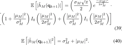
σ2M =p2M+1,M+1(k+ 1, M+ 1), (38)
where pM+1,1:M(k + 1, M+ 1) is a vector containing the
first M entries of the last row of the matrixP(k+ 1, M+ 1)
and pM+1,M+1 is the last entry of the the last row of the
same matrix P(k+ 1, M+ 1). Since˜hM(qk+1)is a complex
Gaussian random variable then first two moments of its modulus are:
Eh|˜hM(qk+1)|
i
=
σM√π
2
e −|µM|2
2σ2
M ·
1 + |µM|
2
σ2
M
I0
|µM|2
2σ2
M
+
|µM|2
σ2
M
I1
|µM|2
2σ2
M
(39)
Eh|h˜M(qk+1)|2
i
=σ2M+|µM|2. (40)
It is interesting to note (compare (39) and (40) with (33) and (34)) that the first two moments of the channel predictor of order M (|˜hM(qk+1)|) have the same form as the two first
moments of the channel predictor of order2(|h˜2(qk+1)|). The
only differences are thatµM 6=µandσM2 6=σ2, see (31), (32),
(37) and (38). Therefore, we can use this similarity to extend the IPPF-2 to derive the IPPF-M with an arbitrary memory order M using the same approach. So we can optimize the IPPF-M atQM(k)andHˆM(k)by solving:
IPPF-M.
max qk+1
θEh|˜hM(qk+1)|n
i
−(1−θ)kqk+1−qkk2
s.t.
2< M ≤k, n= 1,2
(41)
whereθ ∈[0,1], nandM are design parameters. Regarding the memory order parameter M we must mention that to
use the IPPF-M with full memory order we must choose
M(k) =k−1 and so the memory order of the path planner increases at each iteration. Now, similar toIPPF−2−Aif this optimization problem is solved online rather than off-line it becomes easier to solve. But as opposed toIPPF−2−A
the cost function ofIPPF−M(k)has no symmetries and so we do not reduce the search space in the same way. Another difference with IPPF−2−A is that the cost function is computationally more expensive to evaluate8 but as we shall see in section VII its performance is significantly better.
VII. SIMULATIONS
In the simulations, we selected the robot parameters to fit the TOMR used in [2] which describes a real robot. We consider the estimation error to have a varianceσ2
e= 0.05, we
select a wavelengthλ= 14.02cm, corresponding to a carrier frequency of2.14GHz, andT = 833.775ms.
We will first test the path planners with memory order one and compare them with memoryless path planners. So we first consider the following MDAs:
1) MDA1(N): In this MDA the stopping points are prede-termined. They are uniformly distributed along a straight line and the distance between adjacent stopping points is kqk−qk+1k2≈0.3827λ.
2) MDA2(N): This MDA uses an IPPF-1. The distance function used is obtained by solving off-line (12) for
N = 2 withθ= 0.99. In addition we select ψ(k) = 0
so the stopping points will lie into a straight line. 3) MDA3(N): Similar to MDA2(N) but the angle ψ is
optimized according to (13) with θ= 0.9 and for each different number of stopping points variable N. In addition, for reference purposes we plot the upper bound for E[|h(qopt)|2]for the case when the MDA uses predetermined
geometries. This upper bound is reached when all the N
wireless channels considered are independent. This can be confirmed by first taking into account that, from a communica-tions point of view, MDAs with predetermined geometries are mathematically equivalent to the selection combining multi-antenna diversity technique [34] and then taking into account that the performance of such diversity technique is degraded by channel correlation [35].
First of all, the most striking aspect that we observe in Fig. 1 is that the MDA’s using the IPPF-1 surpass E[|h(qopt)|2]
for the case when all the channels are independent. In section IV-B we demonstrated that forN = 2if we use the distance function (11) then the channel gain obtained can be higher than when all the wireless channels are independent. The results in Fig 1 confirm this result and show that this is actually true for any number of stopping points.
Since all the MDAs in [15]-[21] use predetermined ge-ometries then their performance respect to the channel gain obtained is maximized when all the channels are independent. In addition, as we have just observed from Fig. 1 the MDA2
8Because the cost function of IPPF-M(k)depends onµ
M, see (37), and to
calculate this term we first need to calculate the correlation matrixC(k, M)
[image:10.612.52.301.450.542.2]and MDA3 produce higher values ofE[|h(qopt)|2]than when
all the channels are independent. Therefore the MDAs using our path planner with memory order one outperform all the MDAs in [15]-[21] respect toE[|h(qopt)|2]. Also note that the
improvement in E[|h(qopt)|2] for the MDAs 2 and 3 respect
to the case in which all channels are independent comes from the use of the path planner with memory order one that introduces correlation between the channels only in certain cases. Thus showing that unlike most diversity techniques in which correlation degrades their performance [35] MDAs can improve their performance by controlling the correlation in an intelligent way as we did in the development of the IPPF-1. To the authors knowledge this is the first diversity technique in which correlation has been shown to be beneficial.
From Figs. 1-2 we observe that the MDA2(N)outperforms in terms of E[|h(qopt)|2] and the mechanical energy used
the MDA1(N)(which uses predetermined stopping points ar-ranged along a straight line). Now, the MDA3(N)also uses an IPPF-1 with the same distance function as the MDA2(N)but instead of moving in a straight line it optimizes the direction vectors (seeDirection−OP) and therefore reduces the dis-tance traveled during the selection phase. As we can observe in the figures, in terms of E[|h(qopt)|2] both the MDA2(N)
and the MDA3(N)have practically the same performance but the MDA3(N) uses significantly less mechanical energy due to the reduction in the distance traveled during the selection phase. Now, we observe that for the special case of N = 3
stopping points MDA3(N)produces higherE[|h(qopt)|2]than
MDA2(N). This is because the optimal angle ψ for this particular case is around 120 degrees and so in some cases the resultant geometries match the geometries that would be produced by a path planner with memory order two. Therefore, in this particular case for N = 3, the IPPF-1 used by the MDA2(N)acts as an approximation for an IPPF-2 and this is why MDA3(N)produces betterE[|h(qopt)|2]than MDA3(3).
2 4 6 8 10 12
1.4 1.6 1.8 2 2.2 2.4 2.6 2.8 3 3.2
N
E
[
j
h
(
qo
p
t
)
j
2]
[image:11.612.335.535.55.211.2]Independent channels CP MDA1 CP MDA2 CP MDA3
Figure 1. E[|h(qopt)|2]obtained by the MDAs as a function of the number
(N) of stopping points.
Now, to evaluate the performance of the path planners with memory order two we consider the following MDAs:
1) MDA4(N): This MDA uses an IPPF-2. The IPPF-2 is obtained by solving online IPPF−2−A with θ = 0.99 andn= 1.
2 4 6 8 10 12
0 0.5 1 1.5
N
E
[
Em
ec
h
]
MDA1
MDA2
[image:11.612.74.271.490.644.2]MDA3
Figure 2. E[Em(1, N+ 1)]for different MDAs as a function of the number
(N) of stopping points.
2) MDA5(N): Similar to MDA4(N)but withn= 2. 3) MDA6(N): Similar to MDA5(N)but without the
‘semi-plane alternation’ mechanism mentioned in section V. 4) MDA7(N): This MDA uses an IPPF-2. The IPPF-2 is
obtained by solving online IPPF−2−B with θ = 0.99.
5) MDA8(N): This MDA uses the rule-based path planner with memory order two and the values of its parameters (d,Dandη) are the same ones used for the MDA3(N). Note that this is the path planner with memory order two that we proposed in [22].
Note that IPPF-2s require two stopping points to start working so in order to calculate the second stopping point in the MDAs 4-8 we use the IPPF-1 used in the MDA2(N)and to calculate the remaining stopping points we will use the corresponding IPPF-2.
We observe first in Figs 3-4 that they can outperform the MDAs using IPPF-1. The MDA4(N) uses an IPPF-2 that at time instant tk maximizes E[|˜h(p(tk+1))|]. We observe that
for N = 3 produces approximately the same E[|h(qopt)|2]
as MDA1(3) while using less mechanical energy but then for N > 3 its performance in terms of E[|h(qopt)|2] is
lower than the simple MDA1(N) which uses a memoryless path planner. Now, the MDA5(N) uses a similar IPPF but instead of maximizing at time instant tk E[|˜h(p(tk+1))|]
it maximizes E[|˜h(p(tk+1))|2]. This small difference has a
significant impact on the performance as we can see in Figs. 3-4. For a small number of stopping points it outperforms the MDAs using the IPPF-1 in terms of E[|h(qopt)|2] as
well as in terms of the mechanical energy used. But then for
N > 6 its performance in terms of E[|h(qopt)|2] becomes
lower than the MDAs using the IPPF-1 and even lower than the MDA1(N). Now, the only difference between the MDA5(N)
and MDA6(N)is that the MDA6(N)does not use the ‘semi-plane alternation’ mechanism mentioned in section V. In Fig. 3 we observe that the lack of this ‘semi-plane alternation’ mechanism reduces the performance in terms ofE[|h(qopt)|2]
that increases the correlation among the channels and therefore reducesE[|h(qopt)|2]. This shows the benefits of introducing
the ‘semi-plane alternation’ mechanism into the IPPF-2. As we mentioned, MDA4(N) uses an IPPF-2 that maxi-mizes the gain of the channel predictor while MDA5(N)uses an IPPF-2 that maximizes the power of the channel predictor but MDA7(N)uses an IPPF-2 that maximizes a cost function slightly differently, see IPPF−2−B, that does not have a physical interpretation. Nevertheless we can observe in Fig. 3 that in terms of the channel power it outperforms all the previously considered MDAs and in terms of the mechanical energy it uses less energy than the MDAs using the IPPF-1. This suggests that we might find more cost functions for IPPF−2−B that do not necessarily have a physical interpretation but produce better results.
To finish with the analysis of the IPPF-2s we consider the MDA8(N)which uses a rule-based path planner. As we can observe from Figs 3-4 the MDA8(N)has a good performance in terms of E[|h(qopt)|2] and of the mechanical energy used.
For a higher number of stopping points it produces a slightly lowerE[|h(qopt)|2]than the MDAs using the IPPF-1 but uses
considerably less mechanical energy. Now, the MDA8(N)
(which we proposed in [22]) is only outperformed in both aspects by the MDA7(N). Nevertheless the MDA8(N) uses a rule based IPPF-2 which does not require any complex calculation during the MDA execution while the MDA7(N)
uses an IPPF which requires solving an optimization problem at each stopping point thus making it computationally more expensive.
2 4 6 8 10 12
1.6 1.8 2 2.2 2.4 2.6 2.8 3 3.2
N
E
[
j
h
(
qo
p
t
)
j
2]
[image:12.612.335.534.55.212.2]Independent channels CP MDA1 CP MDA3 CP MDA4 CP MDA5 CP MDA6 CP MDA7 CP MDA8
Figure 3. E[|h(qopt)|2]obtained by the MDAs as a function of the number
(N) of stopping points.
Finally we consider MDAs using path planners with arbi-trary memory order:
1) MDA9(N): This MDA uses an IPPF-M(k). The
IPPF-M(k) is obtained by solving online at time instant tk
IPPF−M(k) with θ = 0.99, n = 1 and M(k) = k−1.
2) MDA10(N): Similar to MDA10(N)but withn= 2. As we can observe in Figs. 5-6 the MDA9(N) and MDA10(N) outperform significantly all the previous MDAs in terms ofE[|h(qopt)|2]as well as in terms of the mechanical
energy used. By comparing these MDAs with those using
2 4 6 8 10 12
0 0.5 1 1.5
N
E
[
Em
ec
h
]
Emech MDA1
Emech MDA3
Emech MDA4
Emech MDA5
Emech MDA6
Emech MDA7
Emech MDA8
Figure 4. E[Em(1, N+ 1)]for different MDAs as a function of the number
(N) of stopping points.
an IPPF-2 and an IPPF-1 we note that in general an IPPF with higher memory can have better performance. We also note that MDA10(N)performs better than MDA9(N). From the perspective of E[|h(qopt)|2] this means that the higher
is the memory of the path planner the higher the expected value of the channel power atqopt can be. It is interesting to
note that the IPPFs that maximize the power of the channel predictor perform better than those which optimize the gain of the channel predictor –compare MDA9(N)with MDA10(N)
and MDA4(N)with MDA5(N).
2 4 6 8 10 12
1.5 2 2.5 3 3.5 4
N
E
[
j
h
(
qo
p
t
)
j
2]
[image:12.612.336.535.396.552.2]Independent channels CP MDA3 CP MDA7 CP MDA8 CP MDA9 CP MDA10
Figure 5. E[|h(qopt)|2]obtained by the MDAs as a function of the number
(N) of stopping points.
[image:12.612.73.274.417.572.2]0 2 4 6 8 10 12 0
0.05 0.1 0.15 0.2 0.25 0.3 0.35 0.4
N
E
[
Em
ec
h
]
Emech MDA3 Emech MDA7
[image:13.612.70.273.56.213.2]Emech MDA8 Emech MDA9 Emech MDA10
Figure 6. E[Em(1, N+ 1)]for different MDAs as a function of the number
(N) of stopping points.
network. The channel exhibits small-scale fading and the robot cannot move far from its initial position. Then the robot can execute an MDA using a path planner with memory in order to compensate small-scale fading without moving too much from its initial position. Assume that after some minutes the environment changes then the channel gain observed by the robot may be poor now but it can execute once again the MDA to compensate the small-scale fading.
VIII. CONCLUSIONS
For mobile robots, we showed that mobility diversity algo-rithms (MDAs) using path planners with memory can outper-form (both in terms of mechanical energy used and the channel gain obtained at the optimum stopping point) the MDAs using predetermined stopping points. This important result confirms the superiority of our adaptive path planners. We also derived path planners for any memory order and showed that as the memory of the path planner increases so does the performance of the MDA using it. We also showed that MDAs can take advantage of channel correlation to improve their performance unlike all the other diversity techniques. Future work will extend these results to consider multiples wireless links simultaneously.
REFERENCES
[1] A. H. Nuttall, “Some integrals involving the Q-function” Naval Under-water Systems Center (NUSC) technical report, April 1972.
[2] H. Kim ,B.K. Kim ,“Minimum-energy trajectory planning and control on a straight line with rotation for three-wheeled omni-directional mobile robots”, Proceedings of the IEEE/RSJ International Conference on Intelligent Robots and Systems (IROS), 2012, pp 3119 - 3124. [3] A. Algans, K. I. Pedersen and P. E. Mgensen, “Experimental Analysis
of the Joint Statistical Properties of Azimuth Spread, Delay Spread, and Shadow Fading”, IEEE Journal on Selected Areads in Communications, vol. 20, no. 3, April 2002.
[4] M. Malmirchegini and Y. Mostofi, “On the Spatial Predictability of Com-mucation Channels”, IEEE Transactions on Wireless Communications, vol. 11, no. 3, March 2012.
[5] Y. Mostofi, M. Malmirchegini, and A. Ghaffarkhah, “Estimation of communication signal strength in robotic networks”, in IEEE Inter-national Conference on Robotics and Automation, Anchorage, Alaska, May 2010, pp. 1946â ˘A ¸S1951.
[6] Cruz, Patricio J., and Rafael Fierro. “Towards optical wireless commu-nications between micro unmanned aerial and ground systems”, IEEE International Conference on Unmanned Aircraft Systems (ICUAS), 2015
[7] Kantaros, Yiannis, and Michael M. Zavlanos, “Distributed communication-aware coverage control by mobile sensor networks”, Automatica 63 (2016) pp. 209-220.
[8] Zavlanos, Michael M., Alejandro Ribeiro, and George J. Pappas, “Net-work integrity in mobile robotic net“Net-works”, IEEE Transactions on Automatic Control, vol. 58 no.1, 2013, pp. 3-18.
[9] J. Fink, Jonathan, Alejandro Ribeiro, and V. Kumar, “Robust control of mobility and communications in autonomous robot teams”, IEEE Acces vol. 1, 2013, pp. 290-309.
[10] J. Fink, A. Ribeiro, and V. Kumar, “Robust Cyber-Physical Control of Mobility and Communication in Autonomous Robot Teams”, Proceed-ings of the IEEE, vol. 100, iss. 1, pp. 164-178, 2012.
[11] J. Le Ny, A. Ribeiro and G. J. Pappas, “Adaptive Communication-Constrained Deployment of Unmanned Vehicle Systems”, IEEE Journal on Selected Areas in Communications, Vol. 30 (5), June 2012. [12] F. Meyer et al., “Distributed Estimation with Information-Seeking
Con-trol in Agent Networks”, IEEE Journal on Selected Areas in Commu-nications, vol. 33, no. 11, 2015, pp. 2439-2456.
[13] A. Gonzales-Ruiz and Y. Mostofi, “Cooperative Robotic Structure Map-ping Using Wireless Measurements â ˘A ¸S A Comparison of Random and Coordinated Sampling Patterns”, IEEE Sensors Journal vol. 13, no. 7, July 2013.
[14] A. Gonzalez-Ruis, A. Ghaffarkhah and Y. Mostofi, “An Integrated Framework for Obstacle Mapping With See-Through Capabilities Using Laser and Wireless Channel Measurements”, IEEE Sensor Journal vol. 14, no. 1, January 2014.
[15] D. Puccinelli and M. Haenggi, “Spatial Diversity Benefits by Means of Induced Fading”, 3rd Annual IEEE Communications Society on Sensor and Ad Hoc Communications and Networks, 2006. SECON ’06. [16] D. Puccinelli, M. Brennan and M. Haenggi, “Reactive Sink Mobility
in Wireless Sensor Networks”, Proc. of the 1st international MobiSys workshop on Mobile opportunistic networking 2007.
[17] M. Lindhe, K. H. Johansson abd A. Bicchi, “An experimental study of exploiting multipath fading for robot communications”, Proc. Robotics Science and Systems, Atlanta, GA (June 2007).
[18] J. M. Smith, M. P. Olivieri, A. Lackpour and N. Hinnerschitz, “RF-mobility gain: concept, measurement campaign, and explotation”, IEEE Wireless Communications, vol. 16, no. 1, February 2009.
[19] A. Ghaffarkhah and Y. Mostofi, “Path planning for networked robotic surveillance”, IEEE Transactions on Signal Procesing, vol. 60, no. 7, July 2012.
[20] M.A.M. Vieira, et al., “Mitigating multi-path fading in a mobile mesh network”, Ad Hoc Networks archive Vol. 11, no. 4, June, 2013, pp. 1510-1521.
[21] D. Bonilla Licea, D. McLernon, M. Ghogho and S. A. Raza Zaidi, “Mo-bility Diversity-Assisted Wireless Communication for Mobile Robots”, IEEE Transactions on Robotics, vol. 32, no. 1, 2016.
[22] D. Bonilla Licea, D. McLernon and M. Ghogho,“A mobility diversity algorithm with Markovian trajectory planners”, Proc. of the 23rd IEEE International Workshop on Machine Learning for Signal Processing (MLSP), 2013.
[23] Y. Yuan and Y. Mostofi, “Co-Optimization of Communication and Mo-tion Planning of a Robotic OperaMo-tion under Resource Constraints and in Fading Environments”, IEEE Transactions on wireless communications vol. 12, no. 4, April 2013, pp. 1562-1572.
[24] M. Lindhe and K. H. Johansson,“Communication-Aware Trajectory Tracking”, Proc. IEEE International Conference on Robotics and Au-tomation, Pasadena, CA, USA, May 2008.
[25] M. Lindhe and K. H. Johansson, “Using robot mobility to exploit multipath fading”, IEEE Wireless Communications, vol. 16, no. 1, February 2009.
[26] M. Lindhe and K. H. Johansson,“Adaptive Exploitation of Multipath Fading for Mobile Sensors”, Proc. IEEE International Conference on Robotics and Automation (ICRA), Achorage Convention District, May 2010.
[27] M. Lindhe and K. H. Johansson,“Exploiting multipath fading with a mobile robot”, The International Journal of Robotics Research February 1, 2015 34: 173-200.
[28] S. G. Tzafestas,Introduction to Mobile Robot Control, Elsevier, 2014. [29] R. Siegwart., I.R. Nourbakhsh and D. Scaramuzza, Introduction to
autonomous mobile robots, MIT Press, 2011.
[30] W.C. Jakes, Microwave Mobile Communications, Wiley. IEEE Press, 2011.
[31] D. R. Brian,Spatial Statistics, Wiley Series in Probability and mathe-matical statistics.
[33] G. Dudek and M. Jenkin,Computational Principles of Mobile Robotics. Cambridge University Press, 2000.
[34] A. Goldsmith,Wireless Communications, Cambridge University Press, 2005.
[35] M. K. Simon, M. Alouini,Digital Communication over Fading Chan-nels, John Wiley & Sons, In., 2005.
PLACE PHOTO HERE
Daniel Bonilla Licea received his telematics en-gineering degree from the Unidad Profesional In-terdisciplinaria en Ingenieria y Tecnologias Avan-zadas, UPIITA, Mexico, in 2009. He received his M.Sc. degree in communications from the Centro de Investigacion y Estudios Avanzados, CINVESTAV, Mexico City, in 2011. From May 2011 until June 2012, he did an internship in the signal processing team of Intel Labs in Guadalajara, Mexico. From September 2012 to the present day he has been doing a PhD at the School of Electronics and Electrical Engineering, University of Leeds, U.K.
PLACE PHOTO HERE
Des McLernonreceived his B.Sc in electronic and electrical engineering and his M.Sc. in electronics, both from Queen’s University of Belfast,N. Ireland. He then worked on radar research and development with Ferranti Ltd. in Edinburgh, Scotland, and later joined the Imperial College, University of London, where he received his Ph.D.in signal processing. After first lecturing at South Bank University, Lon-don, UK, he moved to the School of Electronic and Electrical Engineering at the University of Leeds, UK, where he is a Reader in Signal Processing. His research interests are broadly within the domain of signal processing for communications, in which area he has published over 280 journal and conference papers.
PLACE PHOTO HERE
![Figure 2. E([Em (1, N + 1)] for different MDAs as a function of the numberN) of stopping points.](https://thumb-us.123doks.com/thumbv2/123dok_us/7732536.163119/11.612.74.271.490.644/figure-em-different-mdas-function-numbern-stopping-points.webp)
![Figure 4. E([Em (1, N + 1)] for different MDAs as a function of the numberN) of stopping points.](https://thumb-us.123doks.com/thumbv2/123dok_us/7732536.163119/12.612.335.534.55.212/figure-em-different-mdas-function-numbern-stopping-points.webp)
![Figure 6. E([Em (1, N + 1)] for different MDAs as a function of the numberN) of stopping points.](https://thumb-us.123doks.com/thumbv2/123dok_us/7732536.163119/13.612.70.273.56.213/figure-em-different-mdas-function-numbern-stopping-points.webp)
