data
.
White Rose Research Online URL for this paper:
http://eprints.whiterose.ac.uk/131840/
Version: Published Version
Article:
Barthorpe, R.J. orcid.org/0000-0002-6645-8482 and Worden, K.
orcid.org/0000-0002-1035-238X (2017) On multi-site damage identification using
single-site training data. Journal of Sound and Vibration, 409. pp. 43-64. ISSN 0022-460X
https://doi.org/10.1016/j.jsv.2017.07.038
© 2017 The Authors. Published by Elsevier Ltd. This is an open access article under the
CC BY license (http://creativecommons.org/licenses/by/4.0/).
[email protected]
https://eprints.whiterose.ac.uk/
Reuse
This article is distributed under the terms of the Creative Commons Attribution (CC BY) licence. This licence
allows you to distribute, remix, tweak, and build upon the work, even commercially, as long as you credit the
authors for the original work. More information and the full terms of the licence here:
https://creativecommons.org/licenses/
Takedown
If you consider content in White Rose Research Online to be in breach of UK law, please notify us by
On multi-site damage identification using single-site training
data
R.J. Barthorpe
n, G. Manson, K. Worden
Dynamics Research Group, Department of Mechanical Engineering, University of Sheffield, Mappin Street, Sheffield S1 3JD, United Kingdom
a r t i c l e
i n f o
Article history:
Received 7 December 2016 Received in revised form 30 June 2017
Accepted 21 July 2017 Available online 29 July 2017
Keywords:
Structural health monitoring Support vector classification Multi-site damage identification Statistical pattern recognition
a b s t r a c t
This paper proposes a methodology for developing multi-site damage location systems for engineering structures that can be trained using single-site damaged state data only. The methodology involves training a sequence of binary classifiers based upon single-site damage data and combining the developed classifiers into a robust multi-class damage locator. In this way, the multi-site damage identification problem may be decomposed into a sequence of binary decisions. In this paper Support Vector Classifiers are adopted as the means of making these binary decisions. The proposed methodology represents an advancement on the state of the art in the field of multi-site damage identification which require either: (1) full damaged state data from single- and multi-site damage cases or (2) the development of a physics-based model to make multi-site model predictions. The potential benefit of the proposed methodology is that a significantly reduced number of recorded damage states may be required in order to train a multi-site damage locator without recourse to physics-based model predictions. In this paper it is first demonstrated that Support Vector Classification represents an appropriate approach to the multi-site damage location problem, with methods for combining binary classifiers discussed. Next, the proposed methodology is demonstrated and evaluated through application to a real engineering structure–a Piper Tomahawk trainer aircraft wing–with its performance compared to classifiers trained using the full damaged-state dataset.
&2017 The Authors. Published by Elsevier Ltd. This is an open access article under the CC
BY license (http://creativecommons.org/licenses/by/4.0/).
1. Introduction
Structural Health Monitoring (SHM) refers to the process of measuring and interpretingin situdata acquired from a structural system in order to objectively quantify the condition of the structure. SHM has the potential to offer substantial economic and life-safety benefits for aerospace and civil structures in applications as diverse as civil and military aircraft, civil infrastructure, energy generation and offshore structures. The three motivating aspects for SHM that are recurrently mentioned in the literature are: (1) the life-safety benefits achievable through being able to continuously monitor safety-critical components. (2) the economic benefits achievable through avoiding unplanned down-time and increasing the ef-ficiency of inspection and maintenance, and (3) the ability to optimise newly designed structures for which the current health condition is known through monitoring[1]. The damage identification problem can usefully be considered as a hierarchical process, developed from that discussed by Rytter[2], that progresses from the detection of the occurrence of
Contents lists available atScienceDirect
journal homepage:www.elsevier.com/locate/jsvi
Journal of Sound and Vibration
http://dx.doi.org/10.1016/j.jsv.2017.07.038
0022-460X/&2017 The Authors. Published by Elsevier Ltd. This is an open access article under the CC BY license (http://creativecommons.org/licenses/by/4.0/).
n
Corresponding author.
damage; to localisation of where damage has occurred; to classification of the type of damage that is present; assessment of the damage extent; and finally prediction of the residual life of the system in light of the damage.
The focus of this study is on the second level of this hierarchy - localisation - and in particular the problem of identifying changes in the structure that have occurred at multiple locations. Multi-site damage identification represents an important and challenging problem in SHM but one that has received comparatively little dedicated attention in the literature, with the majority of approaches presented in the literature (see, for example, the extensive reviews in[3,4]) focusing on the identification of single-site damage. The impact of this restriction is clear given that anin situstructure would be expected, over time, to exhibit degradation from its baseline state concurrently at multiple locations. Any practical application of SHM should be able to account for this fact, with systems that do not do so potentially unable to accurately describe the true health state of the structure.
Approaches to Structural Health Monitoring may be broadly separated into two classes: data-basedapproaches that follow a statistical pattern recognition paradigm and rely solely on experimental data; andmodel-basedapproaches that make use of the predictions of a representative physics-based model of the structure, typically by applying a Finite Element (FE) model updating procedure. While the problem of multiple damage location from a purely data-based perspective has received very little dedicated attention in the literature, FE model updating is, at least in principle, appropriate to the multiple damage location task. The solution procedure typically involves minimisation of residuals between damage-sen-sitivefeaturesdrawn from the experimental structure and the predictions of the model. Ruotolo and Surace[5]presented an early study of this type focusing on multiple damage location and assessment in a cantilever beams, with a weighted sum of modal features (natural frequencies, modal curvatures and mass-normalised modeshapes) adopted as the objective function to be minimised. A similar approach, the Multiple Damage Location Criterion (MDLAC), is presented by Contursi et al[6], with the cross-correlation between measured and theoretical natural frequencies adopted as the objective function and applied to multi-site damage. An incremental development of the MDLAC approach is presented in[7]with damage location pursued using Dempster-Shafer evidence theory, allowing fusion of the results of frequency MDLAC and modeshape MDLAC outcomes, and a micro-search genetic algorithm used to estimate damage extent.
Dealing with the uncertainty that arises from physical variability, experimental variability and model-form error presents a major issue for FE updating approaches. In recent years this has led to increased interest in methods that explicitly account for uncertainty, with both probabilistic methods (for example Bayesian updating[8,9]), and non-probabilistic methods (for example fuzzy updating[10]) methods demonstrating considerable success for single-site damage location. Nonetheless, challenges remain. The principal drawback of the approach is that developing a finite element model of a complex en-gineering structure sufficient to reliably predict response changes due to damage is a difficult and potentially expensive task, as evidenced by growth of interest in the fields of model validation and uncertainty quantification within structural dy-namics. Secondly, a potentially onerous number of model executions may be required to fully explore the parameter space during the updating step, although approaches such as parameter subset selection may go some way towards addressing this[11]. It is noted that in cases where experimental examples have been used to illustrate approaches they have typically exhibited a low level of complexity, for example cantilever beams and truss-type structures. It is also noted that appro-priately thorough consideration of the impact of numerical and experimental uncertainty remains comparatively rare.
Data-based methods–as typically applied–initially appear less well suited to the multi-class damage location task than model-based methods. Damage location via a statistical pattern recognition (SPR) paradigm requires the adoption of a supervised learning approach, thus requiring the gathering of data from the structure in both its undamaged and damaged state [12]. Localisation is pursued by evaluating the difference between the current state of the structure and an initial baseline state that is representative of the undamaged structure. A feature vector is thus formed that may be compared to previously acquired, labelled observations in order to diagnose the state of the structure by applying a classification algo-rithm. The major drawback of the data-based approach to SHM is the requirement to have access to structural data for all damage states of interest, which is rarely available even for single-site damage. However, a major advantage of this approach is in the handling of uncertainty. Provided the training set contains data representative of the variability that will be seen in the monitoring phase, this variability will be accounted for be any appropriately trained classifier. Manson et al[13]present one such successful example of single-site damage location based upon features drawn from transmissibility spectra, with classification performed using artificial neural networks (ANNs). It is noted that there is a caveat to the requirement for damage state data in cases where the adopted feature exhibits sensitivity to local damage, and some success has been reported using, for example, modeshape curvatures[14]. Nonetheless, such features exhibit disadvantages alongside ad-vantages (susceptibly to experimental noise being an example in the case of modeshape curvatures) and there is clear motivation for developing methods for multi-site damage location that maintain generality of feature choice.
continuous structure or discrete components of an assembled structure. In order to locate single site damage, a supervised learning algorithm would require data from all ten damage states, plus the normal condition. If, instead, data were required to train a classifier capable of locating damage at up to three sites, test data from 175 combinations of damage states would be required. A classifier capable of handling all 210combinations would require data from all 1024 damage states. As
da-maged state data for even single site damage is very rarely available, it would appear unwise to rely on the availability of damage data for all possible combinations of damage location in the general case. It is apparent that the lack-of-data problem, a major obstacle in the diagnosis of single-site damage, is a potentially critical issue in multiple-site damage location.
The contribution of the current study is to present a purely data-based approach to multi-site damage location that dramatically reduces the number of states for which training data is required. This is pursued by constructing a data-driven classifier that is capable of distinguishing occurrences of single-site damage, and evaluating the success of this classifier when presented with multiple-site damage data. The study is experimental in nature with the structure used for illustration being the wing of a Piper Tomahawk trainer aircraft. The features used are discordancy measures associated with trans-missibility measurements, and Support Vector Machines (SVMs) are employed for classification. The layout of the paper is as follows: the experimental structure and data acquisition process are described inSection 2; an approach for reducing the gathered high-dimensional response data into a low-dimensional feature set is developed inSection 3; the performance of the selected feature set when presented with observations of multi-site damage is evaluated inSection 4; and the use of these features as the basis of a multi-site damage classifier is explained inSection 5. Results and conclusions are presented inSections 6and7.
2. Experimental data acquisition
This section describes the experimental structure used in the study and the test sequence adopted. The raw data used in this study consisted of accelerance frequency response functions (FRFs) gathered from 15 locations on the structure in response to single point excitation. The accelerance FRFs are first converted into acceleration transmissibility spectra, de-scribed further inSection 3.2. A key motivation for the use of transmissibility spectra is that they can, in principle, be estimated without measuring the excitation applied to the structure. This makes them an attractive proposition for eventual practical application where load records are unlikely to be available. Finally, multivariate discordancy measures derived from sections of the transmissibility spectra are adopted as candidate damage sensitive features, described further inSection 3.3.
Throughout the study a great deal of attention was paid to test sequencing, as it is known that decisions made here can have a substantial bearing on the quality of the training dataset, and thus the performance of any classifier trained using this set. Care was taken throughout in order to produce a training dataset that is representative of the conditions under which classification will be sought. For the structure under study, it was felt that the boundary condition variability associated with the removal and replacement of inspection panels was likely to represent the most significant source of random variation in the response spectra. Accordingly, care was taken both to reduce this variability to as great an extent as possible by using a torque-controlled screwdriver and taking care over screw tightening, and to account for the outstanding variability in the recorded data through randomisation.
2.1. Experimental structure and data acquisition
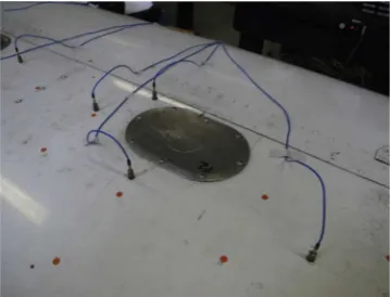
The experimental structure considered in this study is an aluminium aircraft wing, tested in laboratory conditions. The main spar of the wing was bolted in cantilevered fashion to a substantial, sand-filled steel frame that was purpose built for the study as shown inFig. 1. Achieving a truly rigid mounting is non-trivial. However, given the focus on monitoringchanges
in dynamic response as a result of the introduction of damage, it was felt that any small degree of flexibility in the mounting should have minimal effect on the outcome of the study. The wing is mounted upside-down in order to allow access to the inspection panels mounted on the underside of the wing. Mounting the wing in this fashion also ensures that it is preloaded in the correct direction.
Fifteen PCB 353B16 piezoelectric accelerometers were mounted on the upper (as mounted) surface of the wing using ceramic cement. The sensors are denotedS1−S15, with their location plus those of the inspection panels and sub-surface
stiffening elements (dotted lines) shown schematically inFigs. 2and3. The sensors were placed so as to form transmis-sibility paths between sensor pairs, with sensorS14acting as a reference output for sensorsS1-S5andS15performing this
role for sensorsS6-S13. The thirteen resulting paths are indicated inFig. 3and specified in full in Section 3. Placement
directly above stiffening elements was avoided as it was believed that such locations would offer poor observation of localised changes in structural flexibility.
of efficiently delivering low frequency excitation to the structure under test. Five-samples averages were recorded in all cases as this was found to offer a good compromise between noise reduction and acquisition time.
2.2. Damage introduction
In order to introduce damage in a repeatable, and in some sense realistic, way advantage was taken of the presence of inspection panels on the underside of the wing. Five such panels, denotedP1toP5, were employed in the present study, all
of the same dimension and orientation. Through removal of these panels a gross level of damage could be introduced at each location. These damage states are denoted byD{ }. where{ }. indicate the set of panels removed i.e.D{1,5}refers to the
removal of panelsP1andP5. The undamaged case, with all intact panels in place, is referred to asN(normal condition).
Superscripts are used to distinguish repeat realisations of the same damage state e.g.N2refers to the second realisation if
the normal state. Examples of the normal state Nand the damage stateD{ }2 for panel P2 are shown in Figs. 4 and 5
respectively.
[image:5.544.183.365.56.301.2]The advantages of using the removal of a panel as a proxy for damage are that it is non-destructive, repeatable, and the primary effect of panel removal (a localised reduction in structural stiffness) is expected to be similar to the effect of introducing gross damage at the same location. The disadvantage is that the repeatability is not perfect. During preliminary
[image:5.544.164.384.411.500.2]Fig. 1. Piper Tomahawk aircraft wing.
Fig. 2.Schematic of wing inspection panels and stiffening elements.
studies it was found that the removal and reattachment of the panel led to substantial variability in the FRF observations. This and other sources of variability were considered in greater detail prior to the specification of the test sequence in
Section 2.4.
2.3. Sources of experimental variability
Consistent with the aims of the statistical pattern recognition (SPR) paradigm[12], consideration is given to potential sources of variability at the test planning stage. The ultimate aim is to develop a classifier that will generalise well to data unseen during training. By identifying and allowing for sources of variability at an early stage, the prospects of achieving good generalisation at a later stage may be increased. With regard to variability, the objectives of the current study are to reduce variability to whatever extent is possible, and to ensure the remaining variability is appropriately represented in the dataset. Preliminary testing indicated that the panel boundary conditions represented the dominant source of systematic experimental variability, with minimal effects from operational and environmental variation. This is in addition to random variation between runs (i.e. noise).
[image:6.544.180.360.56.193.2]The inspection panels are attached using eight screws. It has been observed in previous studies that the measured FRFs may display marked sensitivity to the boundary condition variability that arises from the removal and reattachment of the panels[13]. The degree of variability observed can be problematic when attempting to construct a sensitive, robust classifier to identify damage states. In the experimental portion of the study, emphasis was placed upon gathering an improved representation of states that would be used for training and validating the developed classifier. To this end, systematic randomisation is applied in the development of the training set test sequence in order to incorporate the effect of panel removal and replacement in the data used for classifier training. In order to reduce the random variability associated with the panel boundary conditions, a torque-controlled electric screwdriver was used for removing and replacing the panels. The order in which the bolts were replaced was also taken into account, with a consistent sequence of attachment main-tained throughout the test. These efforts to reduce random variability were consistently applied for both the training and testing sets. In practical applications, this level of consistency would not be expected. The training dataset should be structured so as to capture the true level of variability as fully as possible, in order that a classifier that generalises well to new data may be built.
Fig. 4.Wing with PanelP2in place.
[image:6.544.180.359.231.369.2]2.4. Test sequencing
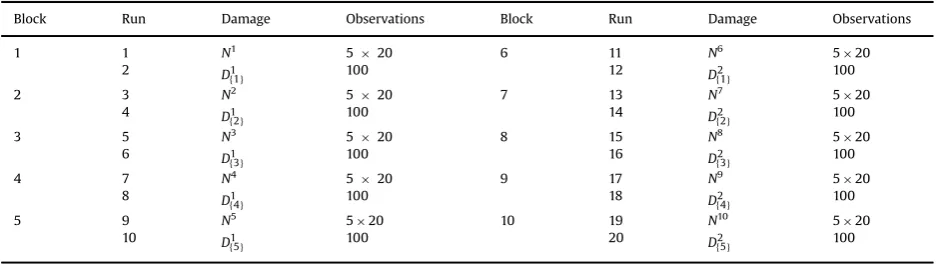
Two tests were conducted, resulting in two data sets being available with which to develop and test classifiers. A test sequence was developed for each test to reflect the differing testing objectives. Randomisation and blocking were applied in the specification of the test sequences in order to account for the effects of measurement noise and panel boundary con-dition variability.
Dataset A comprises 1000 normal state observations and 1000 single-site damage state observations. The primary purpose of Dataset A was to provide training and validation data with which to develop a classifier, with the intention that this classifier then be capable of generalising to identifying multi-site damage for an independent test set. This is a de-manding objective and particular attention was paid to full randomisation of the panel boundary condition in order to fully represent the variability that arises from this effect.Randomisation, as used here, refers to the removal and replacement of panels to ensure that the latent boundary condition variation (that which is present despite the use of a torque controlled screwdriver and care over the order of screw tightening) be represented in the dataset.
The test sequence used for gathering Dataset A is summarised inTable 1. The test consists of 10blocks, each comprising a normal condition run and a single-site damage condition run. For each of the single-site damage states, each block con-tained 20 normal condition runs alternated with 20 damaged condition runs. Eachruncontains 100 observations of five-sample averaged response data. The use of blocks of testing allowed two levels of boundary condition randomisation to be introduced. In order to evaluate the variability arising from single-panel removal within each block, the panel of interest was removed and replaced after every 20 observations for the normal condition runs. Within each block only the panel of interest is removed - the remaining four panels remain in place. For the panel-off case, where there are no single-plate boundary condition effects to consider, a straight run of 100 observations was recorded. Between blocks, all five panels were removed and replaced. This introduced full randomisation of the boundary conditions. In order to add further information, blocks were executed for each of the five panels, and then the sequence repeated.
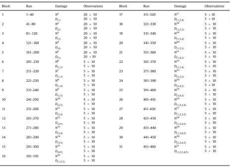
The test sequence used for gathering Dataset B is summarised inTable 2. The primary purpose of Dataset B was to provide a training set to allow the evaluation of the performance of the developed classifiers when presented with new data comprising normal, site and multi-site data. It contains all possible damage states (1 normal condition and 5 single-site damage states plus 26 multi-single-site damage states) plus a number of repetitions for each state with various degrees of randomisation, particularly of the normal condition.
The test was conducted in blocks comprising a number of normal condition runs and runs from one of the damaged state conditions. For each of the single-site damage states, each block contained 20 normal condition runs alternated with 20 damaged condition runs. For the multiple-site damage states, each run contained five normal and five damaged condition runs. Each run contains 10 observations of five-averaged data. Within each block only the panel (or panels) of interest are removed and replaced. For example in the first block, Run 1 compromised 10 observations of the normal conditionN1. Panel
P1was then removed and Run 2, comprising 10 observations of the damaged conditionD1, was recorded. The panel was
then replaced and Run 3, a further 10 observations ofN2, was performed.
Systematic randomisation of boundary conditions through removal and replacement of all panels between blocks was not pursued, although gradual randomisation was introduced as panels were removed and replaced during the test se-quence. This is of some importance to any conclusions drawn with regard to the approach. The primary objective of Dataset B is to provide a training set to allow the evaluation of the performance of the developed classifiers when presented with new data comprising normal, single-site and multi-site data. It is not intended to be the basis of an exhaustive examination of how the developed classifiers perform across the full domain of possible observations, in the presence of variability. Any conclusions drawn must thus include the caveat that they are valid only for the data with which the classifiers were tested; and caution should be employed in drawing general conclusions on the basis of a limited testing dataset.
[image:7.544.40.511.77.209.2]Total testing time was approximately 15 hours distributed over a five day period for Dataset A and 34 hours distributed Table 1
Datatset A test sequence.
Block Run Damage Observations Block Run Damage Observations
1 1 N1
520 6 11 N6 520
2
{ }
D11 100 12 D{ }21 100
2 3 N2 5
20 7 13 N7 520
4
{ }
D12 100 14 D{ }22 100
3 5 N3
520 8 15 N8 520
6
{ }
D13 100 16 D{ }23 100
4 7 N4 5
20 9 17 N9 520
8
{ }
D14 100 18 D{ }24 100
5 9 N5
520 10 19 N10 520
10
{ }
over an eleven day testing period for Dataset B. The observed temperature range was reasonably consistent between the two tests, being 19.2-21.9°C for Dataset A and 19.1-24.8°C for Dataset B. It was not expected that this range of temperatures would have a significant effect on the measured data. In practice, it is to be expected that damage identification would be conducted in the presence of operational and environmental variation, with temperature being among the key drivers in aerospace applications. The robustness of the method in the face of temperature variation was not studied in the current work. In general, three approaches are available for handing confounding influences in data-based SHM: seeking features that are sensitive to damage but insensitive to benign variation; pre-processing the data in such a way that the confounding influences will be filtered out; or including data representative of the confounding influences within the training set. Any practical application of the approach would involve one or more of these approaches to be adopted, and it is the opinion of the authors that every effort should be put into data normalisation where possible with any residual variation subsequently
‘learnt’within the training process. This approach is equally valid whether training is conducted using single-site or multi-site data.
3. Feature extraction and selection
The aim of this section is to describe the reduction of the high-dimensional data recorded inSection 2into a set of low-dimensional features suitable for the training of statistical classifiers inSection 5, and to evaluate the individual performance of the chosen feature set. The objectives of the feature selection and evaluation task may be summarised in several steps.
Extraction of a candidate feature set from raw experimental data. Selection of a low-dimensional feature set containing features that are sensitive to single-site damage, using a training set drawn from Dataset A. [image:8.544.39.510.74.411.2] Evaluation of these features for the identification of single-site damage and multi-site damage using a testing set drawn from Dataset B.Table 2
Datatset B test sequence.
Block Run Damage Observations Block Run Damage Observations
1 1–40 N1
2010 17 311-320 N17 510
{ }
D1 2010 D{1,2,4} 510
2 41–80 N2
2010 18 321-330 N18 510
{ }
D2 2010 D{1,2,5} 510
3 81–120 N3
2010 19 331-340 N19 510
{ }
D3 2010 D{1,3,4} 510
4 121–160 N4
2010 20 341-350 N20 510
{ }
D4 2010 D{1,3,5} 510
5 161–200 N5 20
10 21 351-360 N21 510
{ }
D5 2010 D{1,4,5} 510
6 201–210 N6
510 22 361-370 N22 510
{ }
D1,2 510 D{2,3,4} 510
7 211–220 N7 5
10 23 371-380 N23 510
{ }
D1,3 510 D{2,3,5} 510
8 221-230 N8
510 24 381-390 N24 510
{ }
D1,4 510 D{2,4,5} 510
9 231-240 N9 5
10 25 391-400 N25 510
{ }
D1,5 510 D{3,4,5} 510
10 241-250 N10
510 26 401-410 N26 510
{ }
D2,3 510 D{1,2,3,4} 510
11 251-260 N11
510 27 411-420 N27 510
{ }
D2,4 510 D{1,2,3,5} 510
12 261-270 N12
510 28 421-430 N28 510
{ }
D2,5 510 D{1,2,4,5} 510
13 271-280 N13
510 29 431-440 N29 510
{ }
D3,4 510 D{1,3,4,5} 510
14 281-290 N14 5
10 30 441-450 N30 510
{ }
D3,5 510 D{2,3,4,5} 510
15 291-300 N15
510 31 451-460 N31 510
{ }
D4,5 510 D{1,2,3,4,5} 510
16 301-310 N16 5
10
{ }
Each of these steps is covered in turn. The hypothesis of this section is that it may be possible to find features that offer a good level of discrimination between multiple-site damage states, despite only single-site damage states being available for feature selection.
3.1. Feature extraction
Damage leads to the dynamic response of the structure deviating from that observed when it is in its initial, undamaged condition. The structural response features considered in this study are transmissibility spectra. By comparing examples of undamaged and damaged spectra, regions of the spectra that are sensitive to particular damage states may be identified. These regions form the basis of features that may subsequently be used to train a statistical damage classifier. In the in-terests of developing a statistical classifier, it is desirable that the feature set used is of low dimension. Achieving a suitably concise feature set requires further condensation of the identified spectral region. In this study the additional data reduction is performed using a discordancy measure - the Mahalanobis squared distance (MSD) - between the newly presented and therefore potentially damaged state, and the previously recorded undamaged state. The resulting features are the dis-cordancy values associated with damage sensitive regions of the transmissibility spectra. InSection 5, classifiers are trained using observations of the resulting concise set of damage sensitive features.
The raw data recorded inSection 2comprised 15 accelerance FRFs, each containing 4097 spectral lines. The procedure undertaken for reducing this high-dimensional data to a low-dimensional set of features in this study is as follows. The FRF data are first converted into transmissibility spectra, which have been shown to perform well in similar damage identifi-cation scenarios[15,16,13,17]. In this study, log magnitude transmissibility spectra are employed, which exhibit further useful properties when employed for feature selection, as discussed below. Next, regions of the transmissibility spectra that are sensitive to damage at a particular location are selected. In this instance, feature selection is performed manually on the basis of a principled set of objectives and aided by visual tools. Finally, the identified low-dimensional spectral ranges are reduced to a scalar feature value through the application of the MSD measure.
3.2. Transmissibility data
The raw test data comprised real and imaginary components of the accelerance FRFs between the 15 response locations and the single force input from the shaker. Prior to further processing, this data was converted to transmissibility spectra using the relationship,
ω ω
ω ( ) = ( )
( ) ( )
T H
H 1
ij ik
jk
whereHik( )ω is the FRF between input location kand response locationi,Hjk( )ω is the FRF between input locationkand
response locationj, andTij( )ω is the resulting transmissibility spectra between response locationiand response locationj.
Log magnitude transmissibility spectra were generated for the 13 transmissibility pathsT1 5,14− andT6 13,15− .
The sensors were placed so as to form transmissibility‘paths’between sensor pairs. The sensors are arranged into two groups, the first covering panelsP1andP2and the second covering panelsP3,P4andP5. Each group contains areference
sensor which is common to all transmissibility paths within the group and a number ofresponsesensors. For the first group the reference sensor isS14and the response sensors areS1-S5; for the second group the reference sensor isS15and the
response sensors areS6toS13, resulting in 13 transmissibility paths. Each panel has either two or three transmissibility paths
associated with it. It is expected that the effects of removing a panel may observed in all spectra to some extent, but that the effect will be most apparent in the spectra associated with that panel.
3.3. Dimensionality reduction
The resulting transmissibility data is very high-dimensional. Each observation comprises 13 spectra, each of which contains 4097 spectral lines, giving a 53261-dimensional dataset. In order to alleviate the curse of dimensionality[18], some degree of dimensionality reduction must be pursued prior to applying pattern recognition methods. In this study, di-mensionality reduction is realised as the selection of damage-sensitive regions of the transmissibility spectra, and the reduction of these multivariate regions to univariate features using a discordancy measure.
Selection of damage-sensitive windows of the spectra is the first stage in reducing the dimension of the recorded data. Further dimensionality reduction is achieved through outlier analysis using a discordancy measure. The discordancy measure employed is the Mahalanobis squared distance, which is a multivariate extension of the univariate discordancy measure. Discordancy measures allow deviations from normality to be quantitatively evaluated.
A brief summary of the technique is given here: the technique is described in[19]and validated for an experimental structure in[15,16,13]. For a multivariate data set consisting ofnobservations inpvariables, the MSD may be used to give a measure of the discordancy of any given observation. The scalar discordancy valueMSDξis given by,
Σ
= ( − ¯ ) ( − ¯ ) ( )
ξ ξ ⊤ − ξ
wherexξis the potential outlier,x¯ is the mean of the sample observations and
Σ
is the sample covariance matrix. The MSDapproach offers a measure of the extent by which a sample differs from the population. The mean and covariance matrix may be deemed either inclusive or exclusivemeasures dependent upon whether they are computed using data where outliers are already present. In this study an exclusive measure in adopted, withx¯ and
Σ
calculated using data from thestructure in its undamaged condition only.
3.4. Feature selection from single-site training data
Feature selection from a spectrum can be done in several ways. It may be performed manually, on the basis of en-gineering judgement; algorithmically, primarily by applying some form of combinatorial optimisation; or a combination thereof. The three approaches are illustrated in[20], with outlier analysis performed on transmissibility spectra from an experimental structure subjected to damage. The aim was to select a set of nine features as inputs to a multi-layer per-ceptron (MLP) classifier. First a manual approach was taken to select 44 candidate features from the full spectral dataset, and from these a further reduction to the required nine features was made on the basis of engineering judgement. Secondly, a Genetic Algorithm (GA) was employed to select an‘optimal’subset of nine features from the manually selected set of 44: an example of a manual/algorithmic approach. Finally, a GA was run to select nine features from the full spectral dataset, with no prior selection of feature ranges. The broad conclusion was that the manual/algorithmic approach worked‘best’for the application presented, followed by the fully algorithmic approach and the fully manual approach. The great benefit of the fully algorithmic approach is in removing the requirement for an exhaustive manual search for candidate features.
In this section, the objective is to select features that are robustly indicative of the removal of panels using observations from Dataset A. Objectively optimal feature selection is not pursued in this instance, although this is discussed as an area of future work. The feature selection method is instead performed manually. This process is guided by a series of con-siderations, and aided by appropriate visualisations. In total, 10 features were selected for each of the five panels.
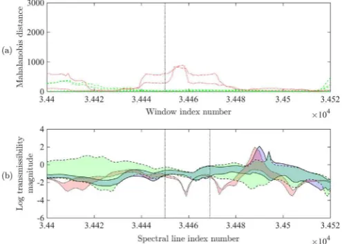
The aim of the feature selection step is to identify features that discriminate between the normal condition and the removal of a single panel, for each of the five panels in turn. For the present work, a predominantly manual feature selection approach was employed, guided by evaluation of the discordancy values of all possible 20-spectral-line windows of the spectra. As each spectrum contains 4097 lines, 4078 such windows existed for each of the 13 spectra, resulting in a total of 53014 candidate features. Discordancy values for each of these features were evaluated using the mean-averaged data recorded for each of the 20 runs in Dataset A. Plotting the discordancy values across the feature set for each of the structural states allows the sensitivity of the features to be visualised. An example for a limited range of the candidate feature set is given inFig. 6(a). The two repetitions of removal of panelP1are shown as red dotted lines. The remaining 18 damage states
(10 normal condition runs and eight other single panel removal runs) are shown as green dashed lines. Four criteria were considered when assessing the strength of a candidate feature.
1. The feature should be sensitive to the removal of the specified panel.
2. In the interests of promoting robustness there should be consistency in the feature values between the two available repetitions.
3. Preferably, the feature should be insensitive to the removal of panels other than that specified. The success of the clas-sifier is predicated upon the discriminative ability of the combined feature set; however, it is expected that if features that are capable of discriminating between damage classes individually can be identified, the discriminative ability of the combined set will also be increased.
4. Preferably, there should be a degree of consistency in the above considerations between the selected feature and those in the immediate vicinity. The feature selection process is guided by a desire to attribute some degree of confidence to the performance of the feature when presented with new data. It would appear, at the very least intuitively, that more confidence may be placed in a feature that is one of several contiguous features that perform well, rather than a feature that performs conspicuously better than its neighbours.
An extended list of candidate features was identified using the MSD plots, with between 15 and 20 features identified for each panel. Each of these features was manually assessed in order to reduce the feature set to a final size of 10 features per panel. Inspection was aided by employing visualisations of the form given inFig. 6.
Fig. 6(a) gives an expanded view of MSD values for the identified feature and for those in its vicinity. The values plotted as red dotted lines are the discordancy values for the window when the panel of interest is removed (panelP1 in the
example plot inFig. 6); the values plotted as green dashed lines are for the normal conditions and removals of the other four panels individually (i.e. panelsP2-P5in the example). The dashed vertical line denotes the selected feature, with the window
index number corresponding to the index of the first spectral line in the 20-line window used to form the feature.Fig. 6
shown in blue and bounded by solid lines. The suitability of candidate features was manually evaluated on the basis of the selection criteria specified above. Through visual inspection of the full range of 4078 candidate windows for each of the 13 spectra, an initial feature set comprising 50 damage sensitive windows was selected.
Returning to the transmissibility plots after initially assessing the features on the basis solely of discordancy values allowed the information set available for making a final decision to be expanded. In several cases, considering the spectra led to some adjustment of the originally identified feature. One example of this is where a greater level of apparent ro-bustness may be achieved through a small adjustment of the window. A second example is where the window returning the highest MSD values is found to contain multiple characteristic structures, such as peaks or troughs in the spectra. In such cases, it may be desirable for the window to span a single peak well, rather than partially span two or more such peaks.
As an example, consider the feature identified inFig. 7. The original feature window, denoted by dotted vertical bars, contained two peaks. In the interests of promoting robustness in the feature set the window illustrated in Fig. 8was preferred to that shown inFig. 7. Despite a lower discordancy value than that for the initially identified feature, plus a lower level of consistency between the two observed repetitions, the feature shown inFig. 8was adopted due to the presence of only one characteristic in the defined window.
Through the process of assisted manual selection detailed above, the feature set was reduced from a candidate set of 53014 features to a final set of 50 features. The results of the feature selection exercise using single-site training data are given inTable 3. For conciseness, only the average discordancy value across the two repetitions is included. Discordancy values were a primary consideration for feature selection, and the values returned in these columns allow the reader some insight into the relative sensitivity of the features to damage on the allotted panel, and to the consistency in values between repetitions.
4. Feature evaluation for single-site and multi-site damage
[image:11.544.149.398.55.238.2]multi-site damage is introduced into the structure. Secondly, the discordancy values associated with each feature are evaluated for all 4600 observations contained in Dataset B. Finally, a summary statistic is applied to allow the discriminative capability of each feature to be concisely stated both for single-site and multi-site panel removal observations.
4.1. Qualitative feature evaluation
An initial assessment of the performance of the features selected inTable 3, when applied to the test set, was made through a qualitative examination of the spectra and through the calculation of discordancy values for every observation in the test set. First, spectral plots were produced to allow the behaviour of the transmissibility spectra in the region of the selected features to be assessed. In order to reduce the number of spectra to be visualised, averaging was applied in a manner consistent with that previously applied for feature selection. For each of the 62 runs (31 normal condition, five single-panel removals and 26 multiple-panel removals) named in the test sequence inTable 2, one mean-averaged spectra was calculated. To aid the clarity of presentation, the interval bounded by the minima and maxima of these averaged runs will be used for illustration inFigs. 9and10in place of the full set of averaged spectra.
Secondly, the feature values returned for each of the 4600 observations in the testing set were quantitatively evaluated. The discordancy valueMSDξfor each feature and for each observation is evaluated using Eq.(2), with the mean vectorx¯and
[image:12.544.148.394.56.236.2]covariance matrix
Σ
representing the normal condition data from Dataset A. Note that while this requires a large number of discordancy evaluations to be made (4600 observations for each of the 50 features in this case, requiring a total of 230000Fig. 7.Feature selection plots for Window Index Number 34456, proposed for identifying removal of panelP4.
[image:12.544.146.394.268.445.2]evaluations), comparative computational efficiency is maintained as the most computationally costly term - the inversion of the covariance matrix–need only be performed once per feature.
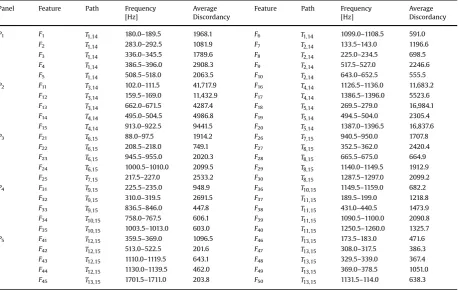
The transmissibility and discordancy outcomes for two of the 50 features are presented inFigs. 9and10. For each feature, four plots are given. The first plot presents the discordancy value data used for selecting features from Dataset A. Removal of the panel of interest is shown using red dotted lines and the removal of the other four panels are shown using green dashed lines. The second plot shows the portion of the transmissibility spectra corresponding to the chosen feature for each of the runs in Dataset A. The intervals spanning single-site removal of the panel of interest is denoted in red; single-site removal of the other panels is shown in green; and normal condition data is given in blue. The third plot shows transmissibility spectra from Dataset B for the chosen feature window. The colour scheme used is as for the second plot, but the intervals now span both single-site and multi-site panel removal. The final plot gives discordancy values for the feature, evaluated for all observations of Dataset B. The plot is divided according to the state of the structure using dashed vertical lines. Observations 1-2300 are for the normal condition; 2301-3300 correspond to single-panel removal; and 3301-4600 correspond to mul-tiple-panel removal. These groups are further delineated using solid vertical lines. Damage states that include removal of the specified panel are highlighted in green.
Fig. 9illustrates featureF32, which performed well in identifying both single-site and multiple-site removals involving
panelP4.Fig. 9(b) illustrates the clear distinction between the removal of panelP4(in red) and the other states included in
Dataset A, and this distinction led to the selection of the feature. Fig. 9(c) illustrates the same feature window for the transmissibility spectra of Dataset B. It is observed that the spectra behave in a very similar fashion to that found for Dataset A, both for the removal of panelP4alone and where panelP4was one of several removed. The clear distinction between the
removal of panelP4and other states is maintained. This is reflected in the discordancy values illustrated inFig. 9(d). The
feature fires strongly for the observations of single panel removal, and similarly strongly for each of the states in which it was one of several panels removed (highlighted with a green background). This very encouraging level of performance was observed for the majority of the 50 identified features, and supports the hypothesis that a good degree of multi-site dis-crimination may be achieved.
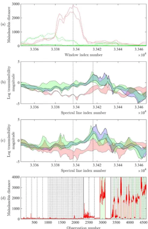
Fig. 10illustrates featureF49, which performed less well in identifying removal of panelP5. While the feature fired to a
reasonable degree for the single-site removals, it was unable to distinguish all of the multiple site damage removals. It was in general found to be more challenging to identify features that performed well for panelP5. However, the reason for
[image:13.544.49.508.78.368.2]featureF49performing less well is likely to be attributable to the nature of the spectra captured within the identified feature
Table 3
Selected feature set.
Panel Feature Path Frequency Average Feature Path Frequency Average
[Hz] Discordancy [Hz] Discordancy
P1 F1 T1,14 180.0–189.5 1968.1 F6 T1,14 1099.0–1108.5 591.0
F2 T1,14 283.0–292.5 1081.9 F7 T2,14 133.5–143.0 1196.6
F3 T1,14 336.0–345.5 1789.6 F8 T2,14 225.0–234.5 698.5
F4 T1,14 386.5–396.0 2908.3 F9 T2,14 517.5–527.0 2246.6
F5 T1,14 508.5–518.0 2063.5 F10 T2,14 643.0–652.5 555.5
P2 F11 T3,14 102.0–111.5 41,717.9 F16 T4,14 1126.5–1136.0 11,683.2
F12 T3,14 159.5–169.0 11,432.9 F17 T4,14 1386.5–1396.0 5523.6
F13 T3,14 662.0–671.5 4287.4 F18 T5,14 269.5–279.0 16,984.1
F14 T4,14 495.0–504.5 4986.8 F19 T5,14 494.5–504.0 2305.4
F15 T4,14 913.0–922.5 9441.5 F20 T5,14 1387.0–1396.5 16,837.6
P3 F21 T6,15 88.0–97.5 1914.2 F26 T7,15 940.5–950.0 1707.8
F22 T6,15 208.5–218.0 749.1 F27 T8,15 352.5–362.0 2420.4
F23 T6,15 945.5–955.0 2020.3 F28 T8,15 665.5–675.0 664.9
F24 T6,15 1000.5–1010.0 2099.5 F29 T8,15 1140.0–1149.5 1912.9
F25 T7,15 217.5–227.0 2533.2 F30 T8,15 1287.5–1297.0 2099.2
P4 F31 T9,15 225.5–235.0 948.9 F36 T10,15 1149.5–1159.0 682.2
F32 T9,15 310.0–319.5 2691.5 F37 T11,15 189.5–199.0 1218.8
F33 T9,15 836.5–846.0 447.8 F38 T11,15 431.0–440.5 1473.9
F34 T10,15 758.0–767.5 606.1 F39 T11,15 1090.5–1100.0 2090.8
F35 T10,15 1003.5–1013.0 603.0 F40 T11,15 1250.5–1260.0 1325.7
P5 F41 T12,15 359.5–369.0 1096.5 F46 T13,15 173.5–183.0 471.6
F42 T12,15 513.0–522.5 201.6 F47 T13,15 308.0–317.5 386.3
F43 T12,15 1110.0–1119.5 643.1 F48 T13,15 329.5–339.0 367.4
F44 T12,15 1130.0–1139.5 462.0 F49 T13,15 369.0–378.5 1051.0
window. The spectra comprise two‘peaks’, only one of which demonstrates a marked shift as a result of damage. This was apparent to some degree from the observations of Dataset A inFig. 10(b), but is more strongly evident inFig. 10(c) for the observations of Dataset B.
The visual assessment of the selected feature windows suggests that there is similarity in the behaviour of spectra due to single-site and multi-site panel removal over some portions of the frequency ranges, and that this behaviour is reflected in the returned feature values. However, the visual assessment of a large number of features is a somewhat onerous task. A concise method for presenting the quantitative evaluation results for the selected features is instead introduced. It should be reiterated that the multiple-site damage data were not used for feature selection.
4.2. Quantitative feature evaluation
The evaluation process generates a large amount of graphical data, and a summary statistic was sought with which to evaluate the discriminatory effectiveness of the selected features. Receiver Operating Characteristic (ROC) curves offer such a measure, providing a simple benefit (true-positive rate) vs. cost (false-positive rate) analysis for two-class data. The area under the ROC curve (AUC) was adopted as a summary statistic for quantifying the discriminative ability of the selected features. A brief introduction to ROC curves and their application to the feature evaluation problem are given here. A more complete introduction to ROC analysis is given in[21].
[image:14.544.146.393.53.433.2]enables the plotting of an ROC curve. The ROC curve may be employed to evaluate the discriminative ability of the data or to select a level for the threshold that is appropriate to the problem.
It is for the first of these functions that it is applied here. As an example, the curve inFig. 11offers an insight into the discriminatory performance of the featureF46, intended to detect the removal of panelP5. A negative class label implies the
panel has not been removed and a positive class label implies that it has. The data used is from the multiple-site damage case. The dashed line corresponds to a classifier offering no discrimination. The further the curve corresponding to a classifier lies above and to the left of this line, the greater its discriminatory performance. In this case, the discriminatory performance of this feature for the data presented may qualitatively be described as good. A quantitative evaluation of the level of discrimination comes from considering the area under the ROC curve.
The area under the ROC curve (AUC) is a simple means of further summarising classifier performance. As the name suggests, the AUC is given by the area lying below the plotted Receiver Operating Characteristic curve (seeFig. 11). The AUC characteristic takes a value in the range [0 1] and has a useful interpretation as the probability that the classifier will rank a randomly selected positive instance higher than a randomly chosen negative instance. For the example of featureF46given
inFig. 11, the AUC value when discriminating between panel-on and panel-off data for Dataset B was 0.778. This is taken to represent a comparatively poor level of discrimination between classes.
For the data considered, the two classes arespecified panel removedandspecified panel not removed. The AUC is adopted as a summary statistic for comparing the classification performance of the individual features in separating normal con-dition data first from single-site data and then from multi-site data.
[image:15.544.149.396.55.430.2]calculated for the discrimination of single-site and multi-site damage for each feature, plus a summary of the overall outcome for each panel, are presented inTable 4.
4.3. Summary of feature evaluation outcomes
The outcome of applying the features selected using the training dataset to the testing dataset may be summarised thus:
A mean AUC value of 0.977 across all features was achieved for the single-site panel removal. A mean AUC value of 0.966 across all features was achieved for the multi-site panel removal. Perfect classification was achieved by 18 of the 50 individual features for single-site panel removal. Perfect classification was achieved by 19 of the 50 individual features for multi-site panel removal.The overall performance of the identified features was deemed to be excellent, with some individual exceptions. Some of the features‘fired’unexpectedly when presented with normal condition observations. A small degree of inter-test variability between Datasets A and B is observed through comparison of normal condition spectra for these features. This finding serves to reiterate the importance of gathering a training set that is truly representative of the conditions that may be encountered.
It is also found that the removal of some of the panels is distinctly more easily detected than the removal of others, and that while some transmissibility paths provide a rich source of features, others offer little discrimination between states. It is notable that transmissibility paths comprising response sensors that are separated from the damage location by a stringer appear to be less successful than those for which the reference sensor is close to the damage. This leads to the suggestion that it may be beneficial to position sensors to be proximal to the expected damage location. In principle, regions of high stress could be predicted via numerical modelling. Of greater practical relevance in situations where such predictions are not available is the further suggestion that for stiffened-panel structures such as the aircraft wing considered, it may be beneficial to place at least one sensor within each panel (panelin this sense being a region of the wing top-sheet bounded on all sides by stiffening elements) that is to be monitored for damage. While these suggestions are perhaps somewhat unsurprising, this is nevertheless a useful demonstration of the importance of sensor placement, and gives some insight into how an extended network of sensors for detecting top sheet damage in similar structures may be formed.
Overall, it was found that the individual features selected on the basis of the training Dataset A (comprising normal and single-site panel removal data) performed very well when presented with single-site panel removal data from a previously unobserved dataset. This result, while expected, serves to validate the test sequencing introduced inSection 2.4.
Of primary interest, however, is the finding that the features also performed very well when presented with multi-site panel removal data, despite no multi-site data being used for feature selection. The multi-site performance of the classifiers averaged over the 50 selected features is very close to that when presented with single-site data, and is evidenced both through visual inspection and through applying quantitative measures. The conclusion drawn is that there is support for the stated hypothesis: for the structure states investigated, it has been possible to find features that offer a high degree of discrimination between multiple-site damage states despite only the single-site damage states having been observed. The significance of this result is the suggestion that the problem of the explosion in the number of damage states that must be observed in order to build a classifier capable of identifying multiple-site damage may be circumvented in some circum-stances. It is, of course, not possible to draw general conclusions on the basis of a single case study, and further investigation into the validity of the approach is warranted.
[image:16.544.179.360.56.200.2]It should be remembered that while evaluating features, the primary concern is that they should fire when damage occurs at the specified location and not fire when the structure is undamaged. It is of only secondary concern that the feature should not fire when damage is not present at the specified location, but is present at other locations on the
structure. If such features are found, it is intuitively easier to interpret the patterns of firing features. However, the appli-cation of statistical pattern recognition methods is specifically intended to reveal underlying patterns within the observed data that would at the very least be challenging for a human observer to interpret.
Having identified features that are individually capable of discriminating between damage states to a good degree, focus moves to the application of statistical pattern recognition in order to employ the features for damage classification. The expectation is that combining the features should offer a further improvement in discriminatory performance. In the fol-lowing section, the features identified form the basis of statistical classification using support vector machines.
5. Multiclass Support Vector Machines
The final stage of the SPR paradigm is the statistical modelling of the selected features. Multiclass support vector ma-chines (SVMs) are investigated for this purpose. The hypotheses to be tested are that:
1. Multiclass SVMs may be an effective option for the classification of multi-site damage data, where observations of each class are available for training, and;
2. That a classifier trained using observations of normal and single-site damage data may offer a level of classification accuracy approaching that of a classifier trained using observations of all damage states. when applied to a testing set that includes multi-site damage observations.
To address these hypotheses two classifiers are constructed and tested. Classifier 1 is trained using data from the structure in all its damage states, including observations of multi-site damage (Dataset B). Classifier 2 is trained using data from the structure only in its normal and single-site damaged states (Dataset A). The objective for both classifiers is to achieve a high rate of correct classification when presented with a testing set of previously unseen data, which contains observations from the structure in single-site, multiple-site and undamaged states. The same architecture is used for both classifiers, and they differ only in the data used for training and validation.
SVMs have been demonstrated to possess several properties that make them well-suited to the damage identification task. They have been shown to generalise well from the small datasets often encountered in damage identification problems, and have the attractive property that they can support different classes of discriminant function (for example linear, polynomial or radial basis functions) without requiring substantial modification of the basic learning algorithm. The multiclass SVM strategy employed in this study is to train a‘one-against-one’binary SVM to identify the occurrence of damage, and an ensemble of
[image:17.544.42.507.78.335.2]‘one-against-all’binary SVMs to locate damage. The structure of the classifier system is described in the following section. Table 4
Area under ROC curve results for Dataset B.
Panel Feature AUC AUC Feature AUC AUC Mean AUC Mean AUC
Single Multi Single Multi Single Multi
P1 F1 0.994 0.989 F6 0.902 0.893
F2 1.000 1.000 F7 1.000 1.000
F3 0.896 0.922 F8 0.999 0.998 0.970 0.970
F4 1.000 1.000 F9 1.000 1.000
F5 0.913 0.901 F10 0.998 0.998
P2 F11 1.000 1.000 F16 0.994 1.000
F12 1.000 1.000 F17 1.000 0.999
F13 1.000 1.000 F18 1.000 1.000 0.999 1.000
F14 1.000 1.000 F19 0.999 1.000
F15 1.000 1.000 F20 0.993 1.000
P3 F21 0.998 0.999 F26 0.999 0.998
F22 0.986 0.984 F27 1.000 1.000
F23 0.996 0.997 F28 0.947 0.983 0.991 0.993
F24 1.000 0.983 F29 0.985 0.991
F25 1.000 1.000 F30 1.000 0.999
P4 F31 1.000 1.000 F36 0.990 0.999
F32 1.000 1.000 F37 0.999 0.999
F33 0.979 0.988 F38 0.994 0.997 0.993 0.997
F34 0.991 0.996 F39 1.000 1.000
F35 0.981 1.000 F40 0.996 0.995
P5 F41 0.999 0.998 F46 0.972 0.986
F42 0.846 0.760 F47 0.991 0.778
F43 0.966 0.983 F48 0.975 0.976 0.933 0.867
F44 0.687 0.794 F49 0.975 0.537
F45 0.973 0.919 F50 0.946 0.941
5.1. Classifier architecture
The classifiers used in this study were created using the MATLAB Support Vector Machine Toolbox. The classification architecture is based upon the binary Support Vector Machine (SVM) extended to the multi-class problem, with each
‘classifier’in fact comprises an ensemble of 6 binary SVM classifiers. The first SVM (labelled SVM1) seeks to separate
da-maged state data from normal state data and thus acts as a damage detection step. SVM1 is unique among the 6 SVMs
employed in being trained using all 50 features identified inTable 3; as all 50 features are sensitive to damage, it is logical to include them all when training the classifier. In principle down-selection could be pursued in order to reduce the dimension of the feature set, but this was not found necessary in the current study.
Five further binary SVMs (labelled SVM2-6) seek to indicate whether removal has occurred for each of the five panels in
turn. Each SVM seeks to class an individual location as‘undamaged’or‘damaged’- SVM2seeks to classify panel 1 as on or off,
SVM3relates to panelP2etc. The classes and features used are summarised inTable 5. During initial development, it was
found that the performance of the individual classifiers SVM2-6was substantially diminished if normal condition data was
included in the training set. As such, training of these classifiers was conducted using a training set comprising damaged state data only. It was also found that greatly improved results were achieved for classifiers SVM2-6 when only the 10
features selected for each panel were used for classification, instead of making use of all 50 features. This agrees with the expectation that the performance of these‘damage location’SVMs may be promoted by restricting them to a space con-taining only those features deemed sensitive to damage at the location of interest.
A key decision in the application of support vector classification is the choice of SVM kernel. The choice of kernel effectively acts as a form of regularisation during training, preventing overfitting to the training data. An initial survey of the feature data indicated that there was a clear argument for adopting a non-linear kernel. In the absence of specific knowledge on the form of the classifying hyperplane, the radial basis function (RBF) kernel was adopted in the discriminant function. This choice was made due to the low degree of parameterisation of the RBF kernel (only two hyperparameters must be set) and its consequent preference for selecting a smooth classification bound. In principle, cross validation could be employed to select between competing kernel options. This was not employed in the current work as it was felt that given the relatively high degree of separability of the data considered this would be unlikely to influence the quality of classification. The data presented to the classifier are log discordancy values. Normalisation of the data is recommended to aid the conditioning of the optimisation problem. In this instance, each feature was normalised to the interval [0 1], with 1 being the maximum value of the feature observed in Dataset A. Where the outcomes of SVM1-6are contradictory, for example
where SVM1indicates no damage has occurred but damage is nevertheless indicated by the location SVMs, precedence is
given to the prediction of the detection classifier SVM1. In cases that damage is indicated to have occurred to the structure,
but damage is not identified at any of the five locations monitored, observations are labelled‘Unclassified’. Classifier 1 and Classifier 2 differ only in the data that is used in their development: all other factors (classifier architecture, validation procedure and features employed) are kept the same. With the structure of the classifiers specified, attention is turned to the data used to train, validate and test the classifiers.
5.2. Training, validation and testing sets
Two experimental datasets are used for developing and testing the classifiers. The first, referred to as Dataset A, com-prises 1000 normal state and 1000 single-site damage state observations of the wing structure. The second dataset, referred to as Dataset B, comprised 2300 normal, 1000 single-site damage and 1300 multi-site damage state observations. Con-ducting supervised learning in a principled fashion necessitates separating the data into three, non-overlapping sets: the testing set, validation set and training set. Each serves a purpose in the development and testing of the classifier.
The training set is used to set the values of the classifier parameters The validation set is used to set the values of the classifier hyperparameters. The testing set is used to verify that the developed classifier works for an independent set of observations.For the RBF kernels employed in this study, two hyperparameters must be set: the misclassification tolerance parameter
[image:18.544.36.504.615.691.2]C, and the radial basis kernel width
α
. The validation step allows an informed decision as to the most appropriate values ofTable 5
Classes and features employed for binary SVMs.
SVM Features employed Positive class Negative class
SVM1 F1 50 All Undamaged Data All Damaged Data
SVM2 F1 10 Damaged,P1removed Damaged,P1not removed
SVM3 F11 20 Damaged,P2removed Damaged,P2not removed
SVM4 F21 30 Damaged,P3removed Damaged,P3not removed
SVM5 F31 40 Damaged,P4removed Damaged,P4not removed