Modeling Steel Corrosion in Concrete Structures - Part 1: A New Inverse Relation between Current Density and Potential for the Cathodic Reaction

Int. J. Electrochem. Sci., 5 (2010) 302 - 313

International Journal of

ELECTROCHEMICAL

SCIENCE

www.electrochemsci.org

Modeling Steel Corrosion in Concrete Structures - Part 1: A

New Inverse Relation between Current Density and Potential

for the Cathodic Reaction

Luc The Ngoc Dao1,*, Vinh The Ngoc Dao2, Sang-Hyo Kim1 and Ki Yong Ann1 1

School of Civil and Environmental Engineering, Yonsei University, Seoul 120-749, Republic of Korea

2

School of Civil Engineering, The University of Queensland, Australia *

E-mail: [email protected]

Received: 6 January 2010 / Accepted: 15 March 2010 / Published: 31 March 2010

Corrosion of steel reinforcement can seriously compromise the service life of reinforced concrete structures. Hence, service life prediction and enhancement of concrete structures under corrosion attack are of significant importance. As a result, numerical methods that can reliably predict the service life of concrete structures have attracted increasing attention. In this, the first of two companion papers, a simple and significantly improved inverse relation relating the current density with potential for the cathodic reaction is proposed. This enables the current densities to be determined accurately from the measured potentials. Equally importantly, the proposed inverse relation also enables the efficient and straight-forward nonlinear algorithm for modeling of steel corrosion in concrete structures to be developed. Such an algorithm is presented in the companion paper of this.

Keywords: Corrosion, Concrete, Numerical modeling, Inverse relation, Cathodic reaction

1. INTRODUCTION

In recent years, numerical methods that simulate the corrosion processes of reinforcing steel in concrete and allow parametric studies in addition to laborious experimental investigations have gained increasing attention [3-6]. This is mainly due to the considerably improved understanding of the basic processes underlying reinforcement corrosion and the significantly increased possiblities for modelling complex electrochemical processes involved in corrosion. However, much remains to be investigated further to fully realise the potentials of current numerical models. Specifically, because of the concentration polarization, the polarized potential of the cathodic reaction expressed as a function of the current density is nonlinear and cannot be solved for explicit inverse relations, which have to be approximated instead. Current approximate inverse relations, however, do not represent well the exact solution. This paper thus aims to propose a new inverse relation between the current density and potential for the cathodic reaction.

2. KINETICS OF CORROSION

2.1. Potential-current density relations for anodic and cathodic reactions

The potential-current density relations for the anodic and cathodic reactions of steel corrosion are well-established [7, 8].

The corrosion of steel in concrete is caused by the dissolution of iron into the pore water at the anode [9], which can be represented by the following half-cell reaction

− +

+

→Fe e

Fe 2 2

(1)

In order for electrical neutrality to be preserved, the electrons produced in this anodic reaction must be consumed at the cathodic sites on the steel surface [9]. The cathodic reaction is given by

− −_→ +

+ H O e OH

O2 2 2 4 4 (2)

2.1.1. Polarization of anodic reaction

The activation polarization of the anodes can be determined by

0 log a a a a i i β η = (3)

where βa is the Tafel slope of the anodic reaction (V/dec), ia is the anodic current density (A/mm2) and

ia0 is the exchange current density of the anodic reaction (A/mm2).

Hence the polarized potential φa (V) of the anodic reaction can be written as [10]

0 0 0 log a a a a a a a i i β φ η φ

φ = + = +

(4)

where φa0 is the equilibrium potential of the anodes (V).

2.1.2. Polarization of cathodic reaction

If the amount of oxygen at cathode is not sufficient, the concentration polarization controls the polarization of cathodes. Concentration polarization at the cathodes can be calculated as

c L L cc i i i zF RT − −

= 2.303 log

η

(5)

where R is the universal gas constant (8.314 J/K.mol), T is the absolute temperature (K), F is Faraday’s constant (9.65.104 C/mol), z is the number of electrons exchanged in the cathodic reaction, ic is the

cathodic current density (A/mm2) and iL is the limiting current density of the cathodic reaction

(A/mm2).

The limiting current density iL of the oxygen reduction at the cathodic sites can be calculated as

follows [7] 3 10 2 2 − = O n O L C t zF D i

δ

where

2 O

D (m2/s) is the effective oxygen diffusion coefficient in concrete, δ (= 0.005 mm) is the thickness of the stagnant layer of electrolyte around the steel surface, tn (=1) is the transference number

of all ions in the solution except for the reduced species, and

2 O

C (mol/l of pore solution) is the concentration of oxygen around the steel.

The activation polarization of the cathodes can be determined as

0 log c c c ca i i β η = −

where βc is the Tafel slope of the cathodic reaction (V/dec) and ic0 is the exchange current density of

the cathodic reaction (A/mm2).

Thus the polarized potential of the cathodic reaction can be written as [10]

0 0

0 log log

303 . 2

c c c c L

L c

ca cc c c

i i i

i i zF

RT

β φ

η η φ

φ −

− −

= + + =

(8)

where φc is the potential (V), and φc0 is the equilibrium cathodic potential (V) under a certain

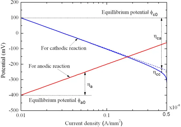
environment. Fig. 1 illustrates the relation between potentials and the current densities for anodic and cathodic reactions given in Eqs. 4 and 8.

Figure 1. Potential-current density relations for anodic and cathodic reactions.

2.2. Inverse relations for anodic and cathodic reactions

In Eqs. 4 and 8, the polarized potentials φa and φc of the anodic and cathodic reactions are

expressed as functions of the current densities. However, in reality, the potentials are usually measured and inverse relations are therefore required to enable the current densities to be determined from the obtained potentials.

in a straight-forward algorithm for modeling of steel corrosion in concrete structures. In addition, the incorporation of a suitable inverse relation also enables a unified algorithm for different types of corrosion modeling, e.g. to solve macro-cell modeling [12-14] and macro-and-micro-cell modeling [11] in one single algorithm. This is presented in detail in the companion paper [15].

2.2.1. For the anodic reaction

The inverse relation of Eq. 4 is the same as the Butler-Volmer relation for the anodic reaction

a a a

e

i

i

φ φ ) ( 303 . 2 0 0 −

=

2.2.2. For the cathodic reaction

Without the concentration polarization term ηcc, the inverse relation of Eq. 8 is similar to the

Butler-Volmer relation for the cathodic reaction

c c c

e

i

i

φ φ ) ( 303 . 2 0 0−

=

However, the effect of concentration polarization on the cathodic reaction often cannot be ignored due to the low oxygen concentration around the cathodic sites on the steel surface. As a result, Eq. 8 becomes nonlinear and cannot be solved for explicit inverse relations, which have to be approximated instead.

Kranc and Sagues [16] attempted to incorporate the concentration polarization into Butler-Volmer equation as follows

c c c

e

i

C

C

i

O O c β φ φ ) ( 303 . 2 0 0 2 2 −

















=

2 are the concentrations of oxygen in the concrete pore solution and at the steel surface,

respectively. This relation, however, is overly simplistic. Among various shortcomings, the relation fails to reflect the asymptotic nature of the curve at limiting current density iL, an important

characteristic of the current density-potential curve for cathodic reaction.

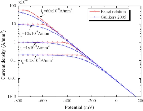
A comparison of Gulikers’ proposed relation and the exact solution for iL between 0.2x10-8 and

60x10-8 (A/mm2) is given in Fig. 2. The exact solution for the current density is obtained by solving Eq. 8 numerically with known values of ic0, φc0, βc, iL, φc using Brent method [17]. It is clear from Fig.

2 that Gulikers’ relation overcomes the non-asymptotic shortcoming of that proposed in [16]. However, Gulikers’ relation still does not completely represent the inverse relation of Eq. 8, especially in the regions of significant change of slope in the current density-potential curve for cathodic reaction. A better relation that represents more fully the inverse relation of Eq. 8 is therefore needed.

Figure 2. Gulikers’ relation with exact inverse relation.

3. NEW INVERSE RELATION BETWEEN CURRENT DENSITY AND POTENTIAL FOR THE CATHODIC REACTION

Upon close examination of the potential-current density relation for cathodic reaction in Eq. 8 and Fig. 2, the following features can be observed

i. When the limiting current density iL of the cathodic reaction is significantly larger than the

cathodic current density ic, i.e. iL/(iL-ic)≅ 1, the concentration polarization is negligible,

resulting in the familiar Butler-Volmer relation for cathodic reaction as in Eq. 10.

ii. When the polarized potential of the cathodic reaction φc approaches the equilibrium cathodic

potential φc0, the cathodic current density ic approaches the exchange current density of the

cathodic reaction ic0.

iii.When the polarized potential of the cathodic reaction φc approaches negative infinity, the

cathodic current density ic reaches the limiting current density iL (asymptotic nature of the

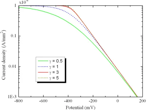
Based on the above observations, a number of modified current density-potential relations for cathodic reaction have been investigated, among which the following relation provides the desired shape of the cathodic curves

γ γ β φ φ γ β φ φ 1 ) ( 303 . 2 0 ) ( 303 . 2 0 0 0 1                                 +         = − − L c c c i e i e i i c c c c c c (13)

where γ is a curvature-defining constant. Fig. 3 illustrates the change of curvatures of the cathodic curves with different values of γ.

Figure 3. Effect of γ constant on the curvature of cathodic curves.

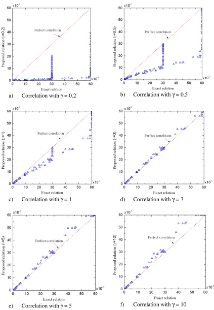
In order to determine the appropriate value for the constant γ, a sensitivity analysis is carried out by comparing the current densities determined by the exact relation and the proposed relation for a typical input data set and for a range of γ. Again, the exact solution for the current density is obtained by solving Eq. 8 numerically with known values of ic0, φc0, βc, iL, φc using Brent method.

Based on the common values of parameters ic0, φc0, βc, iL and φcfor steel corrosion in concrete

structures (Table 1), the input parameters for the sensitivity analysis are selected and given in Table 2. The resulting current densities determined by the exact and proposed relations for different values of γ

a) Correlation with γ = 0.2 b) Correlation with γ = 0.5

c) Correlation with γ = 1 d) Correlation with γ = 3

e) Correlation with γ = 5 f) Correlation with γ = 10

Table 1. Review of parameters for cathodic curve.

ic0(A/mm2) φc0(mV) βc(mV/dec)

Kim and Kim [11] 0.0006x10-8 160 176.3

Isgor and Razaqpur [12] 0.0006x10-8 160 160

Ghods, Isgor and Pour-Ghaz [18] 0.001x10-8 160 160

Kranc and Sagues [16] 0.000625x10-8 160 160

Pour-Ghaz, Isgor and Ghods [13] 0.001x10-8 160 180

Warkus, Raupach and Gulikers [19] - - 200

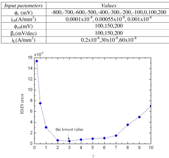
Table 2. Selected input parameters for sensitivity analysis.

(Note: the combination of different values of ic0, φc0, βc, iL, φc provided in following table

gives 891 data points)

Input parameters Values

φc (mV) -800,-700,-600,-500,-400,-300,-200,-100,0,100,200 ic0(A/mm2) 0.0001x10-8, 0.00055x10-8, 0.001x10-8

φc0(mV) 100,150,200

βc(mV/dec) 100,150,200

iL(A/mm2) 0.2x10-8,30x10-8,60x10-8

Figure 5. Variation of Root-Mean-Square error with γ.

In order to find the optimal value of γ, the variation of Root-Mean-Square error, defined in Eq. 14, with γ is plotted in Fig. 5.

(

)

n i i error

RMS

n

proposed c exact c

∑

= 1

2

where i_cexact and i_cproposed are current densities determined by the exact and proposed relations, respectively, and n is the number of data points (n=891).

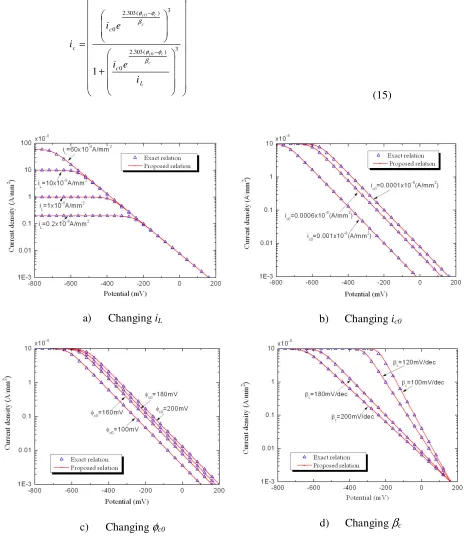
It is clearly evident from Fig. 5 that the optimal value of γ is 3, and hence the proposed relation becomes 3 1 3 ) ( 303 . 2 0 3 ) ( 303 . 2 0 0 0 1                                 +         = − − L c c c i e i e i i c c c c c c β φ φ β φ φ (15)

a) Changing iL b) Changing ic0

c) Changing φc0 d) Changing βc

The validity of this proposed relation is further demonstrated by the following illustration. Let’s consider a typical base case (Table 1) of ic0 of 0.001x10-8 (A/mm2), φc0 of 160 (mV), βc of 180

(mV/dec), and iL of 10x10-8 (A/mm2). Each of these parameters is varied in turn within its common

range (Table 1), while the others remain unchanged. The resulting potential-current density curves are presented in Fig. 6. In all cases, the prediction by the proposed relation correlates very well with the exact solution, confirming the capability of the new relation between current densities and potentials for cathodic reaction.

4. CONCLUSIONS

In this paper, a new inverse relation that relates the current density with potential for the cathodic reaction has been proposed. Besides its desirable simple nature, the proposed inverse relation has been clearly shown to correlate very well with the exact solution.

The significantly improved inverse relation proposed enables the current densities to be determined accurately from the measured potentials. Equally importantly, the proposed inverse relation also enables the efficient and straight-forward nonlinear algorithm for modeling of steel corrosion in concrete structures to be developed. Such an algorithm is presented in the companion paper of this.

ACKNOWLEDGEMENTS

The authors would like to thank Concrete Corea for the support in finance for this research. Mr L.T.N. Dao specially thanks Prof H.W. Song for his sincere support and valuable advice in setting up this study.

References

1. S.L. Amey, D.A. Johnson, M.A. Miltenberger, and H. Farzam, ACI Structural Journal, 95 (2) (1998) 205.

2. K.Y. Ann and H.-W. Song, Corrosion Science,. 49 (11) (2007) 4113.

3. J. Gulikers, Corrosion in reinforced concrete structures, CRC Press (2005) 71. 4. S.C. Kranc and A.A. Sagüés, Corrosion Science, 43 (7) (2001) 1355.

5. H.-W. Song, H.-J. Kim, V. Saraswathy and T.-H. Kim, Int. J. Electrochem. Sci., 2 (2007) 341. 6. R.R. Hussain and T. Ishida, Int. J. Electrochem. Sci., 4 (2009) 1178.

7. H.H. Uhlig and R.W. Revie, Corrosion and corrosion control: an introduction to corrosion science and engineering, John Willey and Sons (2008).

8. M.G. Fontana, Corrosion Engineering, McGraw-Hill (1985).

9. J.P. Broomfield, Corrosion of Steel in Concrete: Understanding, Investigation and Repair, E. & F.N. Spon, London (1997).

10.M. Stern and A.L. Geary, Journal of the Electrochemical Society, 104 (1957) 7. 11.C.-Y. Kim and J.-K. Kim, Construction and Building Materials, 22 (6) (2008) 1129. 12.O.B. Isgor and A.G. Razaqpur, Materials and Structures, 39 (3) (2006) 291.

13.M. Pour-Ghaz, O.B. Isgor and P. Ghods, Corrosion Science, 51 (2) (2009) 415. 14.J. Ge and O.B. Isgor, Materials and Corrosion, 58 (8) (2007) 573.

16.S.C. Kranc and A.A. Sagues, Journal of The Electrochemical Society, 144 (8) (1997) 2643. 17.J.D. Hoffman, Numerical methods for engineers and scientists, Marcel Dekker, New York (2001). 18.P. Ghods, O.B. Isgor and M. Pour-Ghaz, Materials and Corrosion, 58 (4) (2007) 265.

19.J. Warkus, M. Raupach and J. Gulikers, Materials and Corrosion, 57 (8) (2006) 614.