18. (p.26, Para. 2) Note that a different interpretation is introduced for w, to aid understanding of the derivation of Eqs. (2.27a) and (2.27b), however, w, remains a normalised weight function.
19. (p.27) Replace the lowest energy o f all such configurations is added to the data set with the geometry, energy and derivatives o f the configuration with the lowest such energy are added to the data set.
20. (p.30) The confidence radius crad(i) is a defined in Para. 1. Note that this parameter refines the concept expressed in Eq. (2.28) using rad(i).
21. (p.35, Para. 2) Append [8] and found suitable fo r the systems where it is used in this thesis after determined empirically.
22. (p.37) Note to the reader: The numerical trick where the B matrix is
“augmented by zeroes” is used to deal with non-square matrices using SVD because values less than a tolerance (determined by machine accuracy) are set to zero by the procedure (because the reciprocal is too large). Usually, at least one non-zero element on each row would be required to obtain an inverse, however, the SVD procedure is used here to avoid taking the inverse of B or even B’ directly.
23. (p. 39) Note in Section 2.1 that the distortion required to ensure that B’ is invertible is used whenever necessary. As a further note, internal coordinates ensure rotational and translational invariance of the PES.
24. (pp. 41-42) Displacement has been denoted by the vector r in the remaining sections of this chapter, to remove confusion for readers more familiar with conventions used in the references in these sections. Also, note that the
subsections in Section 2.4 define the symbols in order of use, so referring back to an earlier subsection may be necessary.
25. (pp.43-44) Specific references to the Verlet, velocity-Verlet, and shake
algorithms are needed: Use [28], [39] and references therein to review these techniques. Verlet: See L. Verlet, Phys Rev. 159, 98 (1967) and L. Verlet, Phys Rev. 165, 201 (1967). Velocity-Verlet: W. C. Swope, H. C. Andersen, P. H. Berens and K. R. Wilson, J. Chem. Phys. 76, 637 (1982). Shake: W. F. Gunsteren and H. J. C. Berendsen, Mol. Phys. 34, 1311 (1977); and, J. -P. Ryckaert, G. Ciccotti and FI. J. C. Berendsen, J. Comput. Phys. 23, 327 (1977).
26. (pp.45^16) SHAKE should be typeset in small caps: shake.
27. (p.46, Para. 4) Replace whihc with which.
28. (p.46, Para. 4) Append: The prime notation in Eq. (2.74) (and later in Eq. (2.76)) is used to indicate that the summation only includes the constrained bondlengths.
Chapter 3
29. (p.55) Replace reason why with reason that.
30. (p.67) Figure 3.10 has the Intermolecular Separation in Ä.
31. (p.67) Note that the use of J for angular momentum is introduced with the notion of binning trajectories.
32. (p.68) A description of action variables may be found in Ref. 34 (Goldstein, 1980) at the end of Chapter 2.
34. (p.69) Figure 3.11 is shown only as an example of binning, but represents actual results for the vdAWJ PES using 5000 trajectories. The actual number of trajectories is only important for calculating the statistical error using the statistics of proportions defined in any elementary statistical text [20]. The equation for the standard error is represented by (Ne (Nt-N e) / N,3) 12 where Nt is the total number of trajectories and Ne is the number of events. An estimate of the number of trajectories could therefore be deduced from the lengths of the error bars, which is a clearer method of representing the results. 35. (p.71) Sampling of initial conditions is described in Chapter 1, and applies to
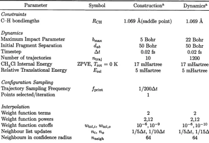
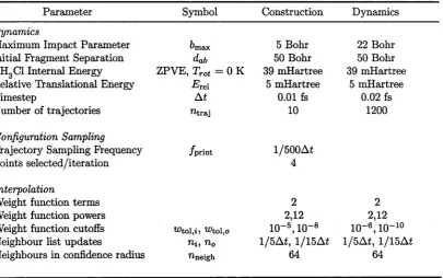
all subsequent chapters. Note that relevant parameters are presented in Table 3.1, and that similar tables are used in subsequent chapters.
36. (p.72, Para. 2) It was sensible to re-use initial conditions (positions and
velocities of the atoms) generated using the analytic PES to run trajectories on the interpolated PES because the interpolated PES would approximate the analytic PES when converged.
37. (p.73) Parameters used in Table 3.1 are described in the text — the Dynamics parameters apply to both the interpolated and the analytic PES.
38. (p.74) Figure 3.15: Note that undulations are due to undulations in the total number of counts.
39. (p.74) The generated MEP is for association of the two monomers. Note that the number of points chosen for the MEP is arbitrary. It is sensible to choose at least a point on the repulsive wall, a point at the minimum and a point at long range. It is also sensible to add further points that were derived while running the minimisation algorithm (in this case steepest descents). Because it is difficult to know, a priori, how the choice of MEP points will affect the number of points required to reach convergence, it makes sense to choose a number that can be feasibly be calculated, including second derivatives, without wasting time that could be spent calculating points constructing the PES. If the MEP point is important to the PES, the methodology should add the point, otherwise it is a waste of computational effort. This PES was deliberately inexpensive to calculate to test the methodology, however, to be a realistic test case, a number that would be sensibly chosen for a modest level of ab initio theory was used: 33. Similar logic is applied to this choice in later chapters.
40. (p.74) The methodology for running the dynamics in Cartesian coordinates using rattle has been provided in Chapter 2.
41. (p.75, Para. 1) Trajectories were inexpensive to run on this system. Thus, only one point is added per iteration. The sampling method was alternated in order to study the effect of each individual point. For this system, a PES was constructed using only RMS sampling and using /?-weight sampling, however, better results were obtained using the alternating method. Until the Bayesian sampling methodology was developed, prior papers for the iterative
construction scheme by Collins and co-workers (see references in Chapters 1 and 2) indicated that a mixed sampling method produced better results, probably because the advantages of each method would offset the
methods and combinations of sampling methods when embarking on a new system. This was done for systems in this work. Results were not presented for initial experimentation because it was not the purpose of this work is not to examine the differences between the sampling methods. As a final
recommendation, if such initial experimentation cannot be afforded, the Bayesian methodology appears to be the state-of-the-art sampling mechanism available at the conclusion of this work.
42. (p.75) Note that points sampled from trajectories for the purpose of estimating errors in the interpolated surface at different times during construction are obtained by performing calculations at configurations printed every fixed number of time steps. The number of time steps between printing
configurations is irrelevant because “enough” trajectories are run. Enough trajectories are run for sampling purposes when the number of samples appears to lead to convergence in the average error. The odd number of geometries, 3481, is simply due to not knowing how many geometries will be sampled for each trajectory (which has a unique set of initial conditions). The number of geometries used to estimate the error is in excess of the number required for the average error to converge. However, since the points had been calculated anyway, there was no harm in using all of them since the remaining calculations are inexpensive because the number of interpolation calculations was only equivalent to a trajectory run for 3481 timesteps or 0.6962 ps for this system.
43. (p.77) Table 3.2: The numbers of points in the interpolated PES chosen to determine cross-sections were simply arbitrary places to stop. Only enough results are shown to demonstrate convergence (for example, results between 255 and 565 added points are clearly not required). A regular spacing was avoided in order to attach any significance to the spacing. It is also obvious that more convergence testing is advisable early in the construction to better estimate the rate of convergence and therefore how often it will be necessary to check convergence afterwards. Note that the rate of convergence,
particularly for reactive systems later in this work, should not be assumed to be a monotonically decreasing function of the number of data points until enough convergence testing has been performed for this conclusion to be likely.
44. (p.77, Para. 2) The error limits for the smaller cross-sections may be “quoted as too small” because the statistics are determined from such a small number of trajectories.
45. (p.78) The accuracy demanded o f the interpolated PES should be interpreted as the error in the PES in dynamically important regions demanded for particular applications. This point is used to raise questions in the following two sentences and is intended to be expanded further in the following chapter where these questions are answered.
Chapter 4
cross-sections that result from exploration of classically forbidden regions of the PES.
47. (p.84, Para. 1) Replace datapoints with data points.
48. (p.85) Note that the spacing of MEP points is shown in Figure 4.3. Again, the number of MEP points was arbitrary. However, a smaller number was chosen than for the previous system because the PES was less anisotropic.
Apparently, this was a good choice because the results in Table 4.1 demonstrate more rapid convergence than was observed in the previous
chapter. It may have been interesting to choose a much more aggressive MEP, such as one containing only three points. Unfortunately, an examination of the behaviour of the methodology under such conditions was not within the scope of this thesis.
49. (p.86) Replace ofspherical with o f spherical.
50. (p.86) m l and m2 in Eq. (4.2) should read niA and mg respectively. 51. (p.88) RATTLE should be typeset in small caps: rattle.
52. (p.88) The RMS sampling method was thought to be more useful in the repulsive wall region of the PES where many closely spaced points would be required to reduce the error in the PES because the energy varies greatly with small changes in configuration. It was also known that anisotropy in the PES in this region at translational energies significantly greater than the depth of the minimum (below infinite separation) would be important to the dynamics
[2]-53. (p89) HYBRIDON should be typeset in small caps: hybridon.
54. (p.89, Para. 4) Green’s work was referenced in the previous paragraph. It is assumed that the reader should again see Ref. 3.
55. (p.90) Replace cases(a) and (b) with cases (a) and (b) (i.e., add space).
56. (p.90) Energies were chosen for comparison with previous work, although the results of previous work are recalculated here with tighter quantum scattering convergence criteria.
57. (p.92) Note that coordinates used in Fig. 4.4 are defined in Fig. 4.2. All coordinates are defined in the introductory section of each chapter. 58. (p.93) Insert space into case(c).
59. (p.95) See (31) for why an odd number (2433) of configurations were sampled. Instead of using classical trajectories, partial wave analysis was used, but the principle behind regular sampling is the same.
60. (p.98) Table 4.4: Replace Ec with Erei for consistency with other chapters. 61. (p.99) A detailed comparison with methods that involved placement of a 40
points on a grid is not provided because the results are quantitatively the same. However, the strengths of the Shepard interpolation that were addressed in Chapter 2 apply here. In addition, it is clear that calculations at grid points will not scale well to larger systems, as described in Chapter 2.
Chapter 5
63. (p. 111, Para. 3) Replace an potential energy with a potential energy.
Chapter 6
64. (p.l 17, Para. 1, last sentence) For clarity, append than HF/3-21+G(d). 65. (p.l 18, Para. 1) Reference for Hase and co-workers: L. Sun, K. Song and
W.L. Hase, Science, 296, 875 (2002).
66. (p.l 19) Reference for Igarashi and Tachikawa: See Ref. [5] and [6].
67. (p. 120) Replace As in previous chapters with in this and subsequent chapters. 68. (p. 121) ZPVE: Zero Point Vibrational Energy.
69. (p. 122) The same parameters were used for unconstrained trajectories as for constrained trajectories because these were still found to be suitable through experimentation.
70. (p. 123,124) More points were selected per iteration for the “unconstrained PES” because it was anticipated that the unconstrained system would be slower to converge. It was also possible to apply additional intuition after the constrained PES was partially constructed.
71. (p. 123,124) ???Alternating sampling was used again to compare the effect of each type of sampling as the PES construction progressed (no significant conclusions could be drawn so such comparisons have not been presented). Note that a discussion of the theory, including the discussion of the generation of initial conditions is discussed in Chapter 2.
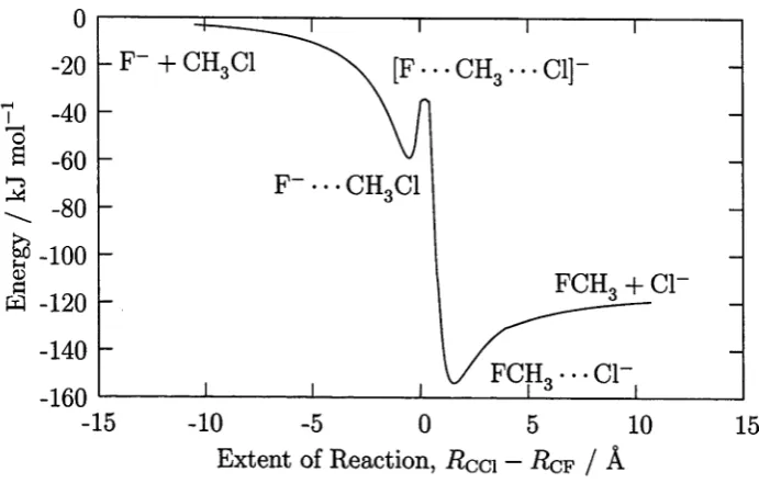
72. (p. 125) For clarity, the data on Fig. 6.2 is shown as a continuous function because there were a large number of points (120 along the MEP). A larger number of points were used than for previous systems because more points were required at long range and it was anticipated that a larger system than previously attempted may require more points in the converged surface. Note that software versions are only listed in the references for brevity.
73. (p. 126) Table 6.3 caption: Replace is shown with are shown. 74. (p.l29, Para. 1) Replace Cl- with Cl'.
75. (p. 130) Figure 6.3 was generated using interpolated energies everywhere on the displayed grid.
76. (p. 137, Para. 1) Ensure that fo r this system is surrounded by commas.
77. (p. 140, p. 141) Figures 6.10 and 6.11: All dynamical parameters, including the number of trajectories (1200) are shown in Tables 6.1 and 6.2. Explicit mention in the text is provided as a reminder, but note that the number of trajectories can be simply derived from the size of the cross-section and the length of the corresponding error bar.
79. (p. 146) Figure 6.15 caption: Replace Langevin cross-section with Langevin rate constant (which does not depend on relative translational energy). 80. (p. 146) Figure 6.15 caption: Add, after the first sentence, The “Total
Reaction” rate constant represents results from this work (with error bars). 81. (p. 147) Note that running backward trajectories was not required for the
unconstrained system because early trajectories sampled the reactive channel very well.
82. (p. 149) Note that for all figures in this chapter (including Fig. 6.17) it has been noted that errors bars are displayed and errors are quoted for two standard deviations.
83. (p. 150) Leaving out ZPVE in the initial conditions for the unconstrained trajectories would not provide a meaningful comparison in this work, because previous studies have investigated the effect o f ZPVE for Sn2 reactions. 84. (p. 152) Space is required to separate terms as in CH3CI + CL.
85. (p. 152) Add after sentence about energy disposal: From the current understanding o f IVR (See Nesbitt and Field, J. Phys. Chem., 100, 12735 (1996)), lowest frequency modes are the best sinks (higher density o f states), however, any energy that should be transferred into the C-H stretching motions is obviously ignored when constraints are used.
86. (p. 153) For clarity: Add. The validity o f the “constrained” PES refers to the fact that the “constrained" PES is always valid fo r performing simulations
that apply the same constraints.
Chapter
787. (p. 161) Software versions (e.g. Gaussian) are provided in the references. 88. (p. 162) Figure 7.3: Note that the direct channel between HOC* and HCO+
should be removed.
89. (p. 163) Note that all necessary theory to understand Table 7.1, including the method o f sampling initial conditions, is provided in Chapter 2. Trajectory end tests check whether or not the fragments are moving apart and if any o f the intemuclear distances exceed
dab-90. (p. 164) ZPVE was defined in (49).
91. (p. 166, 167) Figures 7.4 and 7.5: Note that the number o f MEP points has been included in the legend o f each figure and is therefore not included in each caption. Note that there is a long-range charge-dipole interaction for this system. However, the scales are chosen in these figures to better display the distribution o f points in the interaction region.
92. (p. 168) Figure 7.8: Replace RcF for the x-axis label with Rco- Add: fo r the final PES (1389 points) to the sentence in the caption. The x-axis o f Figure
7.9 was truncated so that the distribution o f points could be more clearly seen (note that it will be shown, later in the chapter, that the PES is already
converged before the maximum extent o f the x-axis).
93. (p. 172) Note that the number o f trajectories used to check convergence has not been included in the figures because this can easily be determined from Table 7.1, and is reflected by the size o f the error bars.
94. (p. 172, Para. 1) Replace less after with more after.
96. (p. 175) Captions for Figures 7.15 and 7.16: Add Results are for the final PES.
97. (p. 181) Figure 7.26 caption: Add Error bars refer to two standard deviations.
98. (p. 185) Add Inspection of the distributions of energy and angular momentum unfortunately yields few clues as to which degrees of freedom are more important to the dynamics.
99. (p. 186, Para. 2) Replace H-H bonds with H-H distances.
Chapter 8
Corrigenda
Chapter 1
Chapter 2
1. (p. 13) Replace “abinitio” with “ab initio” (note use of italics).
2. (p. 13) The reader is encouraged to review Ref. 3 at the end of Chapter 1 for a thorough account of the ab initio methods used in this thesis.
3. (p. 14) Symbols in Eqs (2.6), (2.6) and (2.7) not fully described: • h= Planck’s Constant (h) divided by 2n
• t= time
• y/, </) are wavefunctions; lower case has been used to distinguish these wavefunctions from the total wavefunctions that are additionally a function of the electronic coordinates in Eqs (2.3) and (2.4).
• £n = energy eigenvalue associated with the lower case wavefunctions whereas E was used for the eigenfunctions that were written as a function of electronic coordinates.
Other variables are described earlier in Section 2.1 or in the succeeding paragraph.
4. (p. 16, Para. 3) Remove the comma after When.
5. (p. 16) Ri in Eq. (2.14) is a component of the internal coordinate vector R. 6. (p. 18, Para. 1) Replace the figure with Fig. 2.1.
7. (p. 18) A space is required after the first full stop in Fig.2.1.
8. (p. 19, Para. 1) Remove full stop after previously in previously. [2], 9. (p. 19) Replace E with Erei for consistency.
10. (p.20, Section 2.2.1) Italicise ab initio (latin). 11. (p.21) Replace italicised Z(i) with boldface Z(/).
12. (p.21) Replace in internal coordinates with in internal coordinates, R,j. Other symbols can be deduced by where the defining equations occur in the
corresponding sentences.
13. (p.21) The reader is referred Ref. 18 of Chapter 1 for a description of the relevance of using reciprocal distances for their asymptotic properties. In the same paper, the authors discuss a description of the redundant coordinate problem that is not fundamentally relevant to this thesis, yet is relevant to a description of the PES construction methodology.
14. (p.22) Para. 1. Replace equation reference in normalised weight function in Eq. (2.21) with (2.22).
15. (p.23) Para. 2. Note that i and o are used to distinguish between parameters corresponding to inner and outer neighbour lists, respectively. This
convention has also been used in later chapters.
16. (p.25) For clarity, replace The number o f trajectories can be small, but large enough with The batch o f trajectories must be large enough.
Scalable Iterative Potential Energy Surface
Construction using Constraints
A thesis submitted for the degree of Doctor of Philosophy of The Australian National University
by
A
l e x a n d e rH
am ishD
uncand eclaratio n
I declare that the research, calculations and results that appear in this thesis are solely my own work. Related publications are cited. The chapter on rotational inelastic scattering in hydrogen is based on work published in:
• A. H. Duncan and M. A. Collins, J. Chem. Phys. I l l , 1346 (1999).
Work in the ion-molecule reaction chapters is to be submitted for publication in collaboration with my supervisor, Dr M. A. Collins.
Alexander H. Duncan
a ck n o w led g m en ts
A good friend takes a long time to grow. (John Leonard)
This work is about growing potential energy surfaces. To grow good potential energy surfaces takes time. More about this later. For now I will discuss growing friends.
Many people could be acknowledged in the years that have passed culminating in this thesis. I have had the opportunity to work in a thriving research group with learned colleagues that I have enjoyed associating with not only in the parlance of reaction dynamics but life in general. Ryan and Fiona Bettens, Ron Pace, Damien Kuzek and of course Mick Collins would all remember fondly the lunchtime discus sions about history and politics. Keiran Thompson, Ramzi Kutteh and Michael Smith deserve special mention for their contribution to the general camaraderie in the group during my time there. Others include visiting scholars such as Simon Petrie.
iv
During my candidature as a PhD student I met the love of my life on a volleyball court and married her. Cara has been a continuing source of support. Cara also brought with her the most supportive parents-in-law I could have imagined. I also thank my parents for their unending understanding and support. Without the support of family and friends, 1 could not have grown so much personally.
abstract
Understanding reaction dynamics is central to a deeper understanding of chem istry. The dynamics of molecules as they approach and collide, as bond-breaking and bond-forming takes place, is determined by the molecular potential energy surface (PES).
The PES is simply the total electronic energy of the whole molecule, which depends on the positions of the atomic nuclei. This energy can be calculated accurately using ab initio (first principles) quantum chemistry. However, to study the dynamics of a chemical reaction, we need to know this energy at every relevant configuration of the atomic nuclei.
During a reaction, the molecular geometry changes a great deal as bonds are broken and formed. So the PES is a complicated function of many coordinates which span a large range of values, and cannot feasibly be calculated everywhere using ab initio methods.
vi
C ontents
I P oten tial E nergy Surface C onstruction
1
1 Towards Scalable Potential Energy Surface Construction 2
1.1 Role of the Potential Energy Surface in C hem istry... 2
1.2 Feasible PES Construction for D y n am ics... 4
References... 8
2 Theory 10 2.1 Reaction D y n am ics... 11
2.2 Interpolation of Potential Energy S u r f a c e s ... 20
2.2.1 Shepard Interpolation ... 20
2.3 Sampling Important Regions of the P E S ... 24
2.3.1 Iterative Scheme ... 25
2.3.2 Selection C r ite r ia ... 25
2.3.3 Bayesian A nalysis... 27
2.3.4 Planar and Linear G eom etries... 36
2.4 Constrained D y n a m ic s... 39
2.4.1 Revision of Unconstrained D y n a m ic s... 41
2.5 Numerical Methods for Constrained D ynam ics... 43
2.5.1 R A T T L E ... 44
References... 50
II
R otation al Inelastic Scattering
53
3 Growing a PES for a Constrained System: N2+ N 2 54 3.1 Introduction... 543.2 An Analytic Test P o ten tial... 55
3.2.1 Functional Forms by Expansion in Terms of Scalar Functions 57 3.3 Classical Dynamics on the Analytic Surface ... 67
3.3.1 Classical Dynamics of Rotational Energy T ran sfe r... 67
3.4 Interpolation of the Analytic S u r f a c e ... 71
3.4.1 Computational D e ta ils ... 72
3.4.2 Discussion of Computational R e s u l ts ... 75
3.5 C onclusions... 78
References... 79
4 Quantum Dynam ics for the PES o f a Constrained System: H2+ H 2 81 4.1 Introduction... 81
4.2 T h eo ry ... 83
4.2.1 Placement of Data Points in Configuration S p a c e ... 85
4.2.2 Convergence of the P E S ... 86
C O N T E N T S viii
C O N T E N T S ix
4.3.1 Computational D e ta ils ... 87
4.3.2 Data Location in Configuration Space... 90
4.3.3 Convergence of the Rotational Cross-sections... 93
4.3.4 Energy Dependence of the Interpolated P E S ... 97
4.3.5 Comparisons with Other M ethods... 99
4.4 Summary and Conclusions... 99
References...101
III
Ion-M olecule R eactions
104
5 Ion-M olecule R eaction D ynam ics 105 5.1 The Systems S tu d ie d ... 1055.2 Ion-Molecule Reaction Dynamics ...106
5.2.1 The Langevin M o d e l... 106
5.2.2 The Double-Well Model for Ion-Molecule R e a c tio n s...I l l References...113
6 An Sn 2 Reaction: CH3C1 + F" 115 6.1 Introduction... 115
6.2 Computational D e ta ils ... 120
6.2.1 C o n s tra in ts ... 120
6.2.2 P a r a m e te r s ... 122
6.2.3 Ab Initio C a lc u la tio n s...125
6.2.4 Trajectory E nd-T ests... 128
C O N T E N T S x
6.3.1 Distribution of Ab Initio P o in ts... 129
6.3.2 Complex Form ation... 134
6.3.3 Is the PES A c c u ra te ? ...138
6.3.4 Convergence of Cross-Sections...140
6.3.5 Convergence of Complex Lifetimes ... 141
6.3.6 Energy-Dependence of the Reaction D ynam ics...145
6.3.7 Unconstrained D ynam ics...147
6.3.8 Unconstrained Dynamics on the Constrained P E S ...151
6.4 R em ark s...152
References...154
7 An Eight-Atom System: CH3F-(-HOC+ 157 7.1 Introduction... 157
7.2 Computational D e ta ils ... 160
7.2.1 C o n s tra in ts ... 160
7.2.2 Ab Initio C a lc u la tio n s...161
7.2.3 Construction of the P E S ...162
7.3 Analysis of R esu lts... 164
7.3.1 Unconstrained Dynamics on the Constrained P E S ... 181
7.4 C onclusions... 186
References...187
List of Tables
3.1 PES and Trajectory Parameters: N2 + N2 ... 73
3.2 Inelastic Cross-sections for N2+N2 ... 77
4.1 Cross-sections for para-para Collisions in H y d ro g e n ... 93
4.2 Cross-sections for ortho-ortho Collisions in H y d ro g e n ... 94
4.3 Cross-sections for ortho-para Collisions in H ydrogen... 94
4.4 Energy dependence of H2 4- H2 Inelastic C ross-sections... 98
6.1 PES and Trajectory Parameters: Constrained CH3C1 + F ~ ... 123
6.2 PES and Trajectory Parameters: Unconstrained CH3C1 + F~ . . . 124
6.3 Stationary Point Energies: CH3C1 + F “ ... 126
6.4 Frequencies: CH3C1 + F~ ... 127
List of Figures
2.1 Parameters used to compute cross-sections... 17
3.1 Potential energy as a function of N2-N 2 intermolecular distance . . 57 3.2 Body-fixed coordinates for N2-N 2 ... 59 3.3 Damping functions used in the nitrogen potential where 9 a = 45°,
0°B = 45°, 4>a = 0°, La — 0, L B = 0 and L — 0...62 3.4 Nitrogen potential using only the dispersion part of the radial con
tribution... 63 3.5 Nitrogen potential using only the electrostatic part of the radial
contribution... 63 3.6 Nitrogen potential using only the overlap part of the radial contri
bution... 64 3.7 Nitrogen potential as a function of one azimuthal coordinate 9a and
R for fixed 0B = 135° and <j>A = 0°... 65 3.8 Nitrogen potential as a function of one azimuthal coordinate 9a and
R for fixed 9b = 45° and 4>a = 0°... 66
3.9 Nitrogen potential as a function of one azimuthal coordinate 9a and
R for fixed 9B = 90° and (j>A = 0°... 66
LIST OF FIGURES____________________________________________ xiii
3.11 Angular momentum in scattered N2 m o lecu les... 69
3.12 Fraction of all N2 + N2 trajectories as a function of impact parameter 70 3.13 Fraction of trajectories for one type of inelastic collision on the N2 +N 2 PES ... 70
3.14 Labelling of internuclear distances in N2/N 2 ... 72
3.15 Inelastically scattered fraction of all N2 + N2 trajectories as a func tion of impact p a ra m eter... 74
3.16 Average absolute error in the N2 + N2 interpolated P E S ... 76
4.1 Labelling of internuclear distances in H2/H 2 ... 84
4.2 Body-fixed coordinates for H2-H 2 ... 87
4.3 Two dimensional projections of data point configurations for the H2 /H 2 system ... 91
4.4 Interpolation energy for H2 + H2 near the global m in im u m ... 92
4.5 Average absolute interpolation error in the H2 + H2 P E S ... 96
4.6 Interpolation energy for H2 + H2 on the repulsive wall ... 97
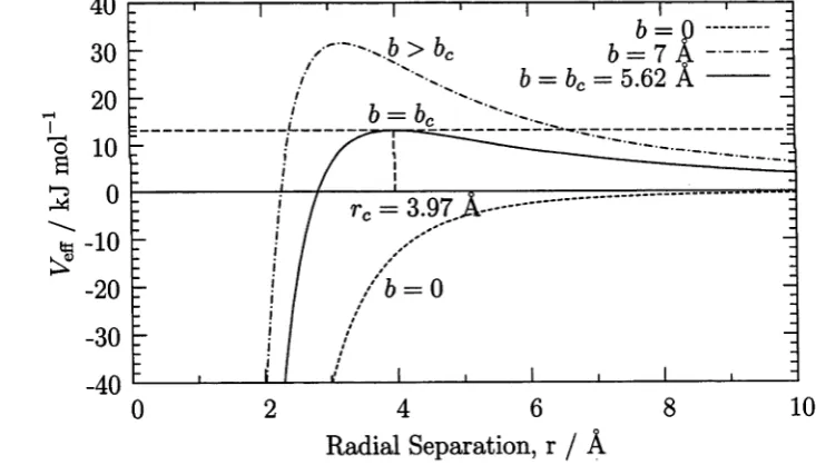
5.1 Effective potential for CH3C1 + F ~ ...108
5.2 Effective potential for CH3F + HOC+ ...109
5.3 Langevin probability of reaction as a function of impact parameter . 109 5.4 Schematic double well energy profile ...112
6.1 Internuclear distances in CH3C1 + F ~ ...120
6.2 Potential energy as a function of extent of CH3C1 + F~ reaction . . 125
6.3 Interpolated potential energy surface for CH3C1+F- ...130
LIST OF FIGURES__________________________________________________xiv 6.5 Distribution of 500 data points added to the CH3C1 + F~ PES . . . 133 6.6 Distribution of 1847 data points added to the CH3C1 + F_ PES . . 133 6.7 Individual CH3C1 + F~ trajectory p a t h s ... 135 6.8 Individual CH3C1 + F- trajectory paths including long range . . . 136 6.9 Average absolute error in the CH3C1 + F- P E S ... 139 6.10 CH3C1+F~ association cross-sections as a function of the number
of data p o i n ts ... 140 6.11 CH3C1 + F “ Sn2 cross-sections as a function of the number of data
p o i n t s ... 141 6.12 Fits for F~ • • • CH3C1 complex life tim es...143 6.13 Fits for FCH3 • • • Cl- complex life tim es... 143 6.14 Fits for F “ • • • CH3C1 complex lifetimes as a function of the number
of data points used in the interpolated PES ... 144 6.15 CH3C1 + F~ substitution rate constants as a function of relative
translational energy... 146 6.16 Average absolute error as a function of the number of data points
in the CH3C1 + F~ PES constructed u n co n strain ed ...148 6.17 CH3C1 + F~ substitution cross-sections for a PES constructed un
constrained ... 149 6.18 CH3C1 + F~ association cross-sections for a PES constructed with
out constraints ... 150 6.19 Interpolated potential about a constrained C-H bond (CH3C1 + F~
P E S ) ...151
LIST OF FIG U R E S xv
7.3 Schematic energy profile for the CH3F + HOC+ r e a c t i o n ...162 7.4 Distribution of 828 additional points added to the CH3F + HOC+
P E S ...165 7.5 Distribution of 150 additional points added to the CH3F + HOC+
P E S ...166 7.6 Distribution of 250 additional points added to the CH3F + HOC+
P E S ...167 7.7 Distribution of 828 additional points at short range in the CH3F +
HOC+ PES data s e t ... 167 7.8 Placement of points in the Rco bondlength coordinate with increas
ing number of data points in the CH3F + HOC+ PES data set . . . 168 7.9 Rc k distance (from HOC+) represented for each data p o in t... 169
7.10 Absolute interpolation errors for the CH3F -I- HOC+ P E S ... 170 7.11 Average absolute energy errors and relative gradient errors for the
CH3F + HOC+ P E S ... 170 7.12 Convergence of CH3F + HOC+ reaction cross-sections with the
number of data points in the P E S ...172 7.13 Convergence of the branching ratio in reactive trajectories with
number of interpolation data points in the CH3F + HOC+ PES . . 173 7.14 Distribution of translational kinetic energy of the products in tra
jectories by CH3F + HOC+ reaction p a t h w a y ...174 7.15 Distribution of angular momentum in the smaller products of tra
jectories by CH3F + HOC+ reaction p a t h w a y ...175 7.16 Distribution of angular momentum in the larger products of trajec
LIST OF FIGURES xvi
7.17 Convergence of kinetic energy distributions for the non-reactive channel with number of data points in the CH3F + HOC+ PES . . 176 7.18 Convergence of kinetic energy distributions for the protonation chan
nel for CH3F + H O C + ...177 7.19 Convergence of kinetic energy distributions for the rearrangement
channel ...177 7.20 Convergence of angular momentum in HOC+ in the non-reactive
channel ...178 7.21 Convergence of CO product angular m o m e n tu m ... 178 7.22 Convergence of HCO+ product angular m o m e n tu m ...179 7.23 Convergence of angular momentum in CH3F in the non-reactive
channel ...179 7.24 Convergence CH3FH+ product angular momentum ... 180 7.25 Convergence of angular momentum in CH3F after HOC+ rearrange
ment ...180 7.26 Cross-sections for each channel for an increasing number of con
straints in CH3F + HOC+ ... 181 7.27 Kinetic energy distributions for the protonation channel with dif
ferent sets of c o n s tra in ts ...182 7.28 Kinetic energy distributions for the rearrangement channel with dif
ferent sets of c o n s tra in ts ...182 7.29 CO product angular momentum for different sets of constraints . . 183 7.30 HCO+ product angular momentum for different sets of constraints . 184 7.31 CH3FH+ product angular momentum for different sets of constraints 184 7.32 CH3F angular momentum after rearrangement: different sets of con
P a r t I
P o te n tia l E n e rg y S u rface
C hapter 1
Towards Scalable P o ten tia l
E nergy Surface C on stru ction
1.1
Role of the Potential Energy Surface in
Chemistry
Understanding reaction dynamics is central to a deeper understanding of chemistry. It encompasses the processes or “physics” that occur in a chemical reaction. The dynamics of molecules as they approach and “collide” is obviously important, as bond-breaking and bond-forming are intimately related to spatial proximity of the reactants. The way the reactants are brought together will depend on the interaction between them: the course of the collision, reactive or non-reactive, is sensitive to the potential energy surface (PES) [1, 2]. The PES describes this interaction as a function of the displacements of all of the interacting particles.
1.1 R o le o f th e P o te n tia l E n ergy S urface in C h em istr y 3
the Born-Oppenheimer approximation implies that the potential energy at any point on one surface can be calculated by fixing the positions of the nuclei, and determining the electronic energy at that configuration.
The electronic energy can be calculated accurately using ab initio theory [3]. Such calculations are a powerful tool for determination of stationary points in the PES, and are useful in characterising chemical reactions and in the calculation of many molecular properties, including electrostatic and spectroscopic properties, for example.
However, to study the dynamics of a chemical reaction, we need to know the potential energy at every relevant fixed position (configuration) of the atomic nu clei. During a reaction, the molecular geometry changes a great deal as bonds are broken and formed. In a classical (molecular dynamics) simulation of a reaction, the energy (and its gradient with respect to nuclear positions) must be calculated at every time step while this large range of configurations is explored.
Quantum simulations might require an even broader range of molecular ge ometries to account for tunnelling in classically forbidden regions. If the chemical reaction dynamics is very sensitive to the shape of the PES, including, for exam ple, the height of some barrier, then very high levels of ab initio theory might be necessary. The computational expense of performing a vast number of high level
ab initio quantum chemistry calculations is prohibitive.
1.2 Feasible PES Construction for Dynamics 4
1.2 Feasible PES Construction for Dynamics
Given that direct use of ab initio calculations is is not feasible, dynamicists have taken different approaches to the determination of accurate PES for dynamical simulations. Usually, a global functional form for the PES is fitted using not only ab initio data but also experimental data. Earlier fitting procedures, such as the diatomics in molecules (DIM) method, LEPS (London, Eyring, Polanyi and Sato) and many-body expansions are reviewed in Ref. 2. Fitting procedures, and the resulting PES, are system-specific and dependent on the type and accuracy of available data. Successful “fits” are therefore performed by experts exercising extensive chemical intuition. Examples are given later in this thesis of different functional forms, as these will be useful in testing new methodology.
Collins and co-workers have developed [4] a scalable iterative method for con structing an interpolated PES using only calculations of the potential energy (and first and second derivatives). The methodology has been applied to many sys tems [5-15], and in each case, only standard quantum chemistry techniques were required. The approach has been successively improved [5-9, 16-18]. Reference 19 provides a recent review of the methodology.
1.2 F easib le P E S C o n stru ctio n for D y n a m ic s 5
The methodology of Collins and co-workers has been extended further through the work in this thesis. Constraints have been used to tackle the dimensionality problem and achieve greater scalability. The theory underlying the methodology of Collins and co-workers will be presented in Chapter 2. The iterative scheme is presented in detail, along with modifications to facilitate the use of constraints in PES construction.
We begin testing the new methodology for systems of four atoms in Chapters 3 and 4. These are small test cases for which reduced-dimensionality functional forms for the PES are available. To test the methodology, we will use the iterative scheme to approximate the functional form PES using interpolation between “data points” determined from the functional forms. Convergence of the interpolated PES can be directly observed by comparing the dynamics described by the interpolant with those described by the functional form. In the first system, we take the opportunity to examine a non-reactive energy transfer process (not previously examined by Collins and co-workers):
which is presented in Chapter 3. In the second system, presented in Chapter 4, the methodology has been applied to another rotational inelastic scattering example:
Here, we apply the methodology to quantum scattering. It was important to examine the application of this type of PES in quantum dynamics, because only classical dynamics is used in the construction of the PES [20]. PES were later constructed for reactive quantum scattering by Collins, Zhang, and co-workers [21- 23].
N2(Ja) + N2(Jb) —*► N2(J'a ) + N2(Jß) (1.1)
1.2 F easib le P E S C o n stru ctio n for D y n a m ics 6
In Chapters 6 and 7 we turn our attention to reactive systems. In these chap ters, we construct interpolated ab initio PES.
Chapter 6 deals with a simple nucleophilic substitution reaction:
CH3C1 + F- —> CH3F + Cl". (1.3)
Reaction (1.3) is an SN2 reaction familiar from organic chemistry. For the collision energies studied in Chapter 6, long-lived complexes of the reactants and products in reaction (1.3) can be formed. Hence, the methodology was also tested for dynamical observables other than cross-sections — the complex lifetimes.
The accuracy of the interpolation is demonstrated by the convergence of re action cross sections and complex lifetimes to constant values as the size of the interpolation data set increases. The interpolation method must become exact at infinite data density. The feasibility of the method is demonstrated by conver gence at a feasible number of data points. In this chapter, we compare the rate of convergence of the PES, with size of the data set, for surfaces constructed with and without constraints. This indicates the utility of employing constraints in the PES construction.
Chapter 7 presents the only results for an eight-atom system using a method ology based on the iterative scheme of Collins and co-workers:
CH3F + HOC+ -> CH3FH+ + CO, and (1.4)
-+C H 3F + HCO+. (1.5)
1.2 Feasible PE S C onstruction for D ynam ics 7
References
[1] D. G. Truhlar, editor. Potential Energy Surfaces and Dynamics Calculations. Plenum Press, New York, USA, 1981.
[2] J. N. Murrell, S. Carter, S. Farantos, P. Huxley, and A. Varandas. Molecular Potential Energy Functions. John Wiley and Sons Ltd, UK, 1984.
[3] W. J. Hehre, L. Radom, P. v. R. Schleyer, and J. A. Pople. Ab Initio Molecular Orbital Theory. John Wiley and Sons, USA, 1986.
[4] J. Ischtwan and M. A. Collins, J. Chem. Phys. 100, 8080 (1994).
[5] M. J. T. Jordan, K. C. Thompson, and M. A. Collins, J. Chem. Phys. 102, 5647 (1995).
[6] M. J. T. Jordan and M. A. Collins, J. Chem. Phys. 104, 4600 (1996).
[7] K. C. Thompson, M. J. T. Jordan, and M. A. Collins, J. Chem.. Phys. 108, 564 (1998).
[8] M. A. Collins and R. P. A. Bettens, Phys. Chem. Chem. Phys. 1, 939 (1999). [9] R. P. A. Bettens and M. A. Collins, J. Chem. Phys. I l l , 816 (1999).
[10] M. A. Collins, S. Petrie, A. J. Chalk, and L. Radom, J. Chem. Phys. 112, 6625 (2000).
[11] M. A. Collins and L. Radom, J. Chem. Phys. 118, 6222 (2003).
[12] R. P. A. Bettens and M. A. Collins, J. Chem. Phys. 108, 2424 (1998). [13] R. P. A. Bettens and M. A. Collins, J. Chem. Phys. 109, 9728 (1998). [14] M. A. Collins and L. Radom, J. Chem. Phys. 118, 6222 (2003).
R E FE R E N C E S 9
[16] M. J. T. Jordan, K. C. Thompson, and M. A. Collins, J. Chem. Phys. 103,
9669 (1995).
[17] K. C. Thompson and M. A. Collins, J. Chem. Soc. Faraday Trans. 93, 871 (1997).
[18] K. C. Thompson, M. J. T. Jordan, and M. A. Collins, J. Chem. Phys. 108,
8302 (1998).
[19] M. A. Collins, Theor. Chem. Ace. 108, 313 (2002).
[20] A. H. Duncan and M. A. Collins, J. Chem. Phys. I l l , 1346 (1999). [21] M. A. Collins and D. H. Zhang, J. Chem. Phys. I l l , 9924 (1999).
[22] M. H. Yang, D. H. Zhang, M. A. Collins, and S. Y. Lee, J. Chem. Phys. 114,
4759 (2001).
C hapter 2
T heory
Knowledge of intermolecular potentials is fundamental to understanding micro scopic properties, which is in turn useful in relating these to macroscopic or bulk properties. It is impossible to determine the potential in detail using experimen tal data alone, although some characterisation of specific regions may be possible. The potential of interacting molecules depends not only on intermolecular displace ment, but also relative orientation. When chemical reaction occurs, the potential energy of the colliding molecules is a very complicated function of the geometry.
2.1 R e a c tio n D y n a m ics 11
2.1
R e a c tio n D y n a m ic s
The motion of a molecule, electrons and atomic nuclei, is determined by the Hamil tonian, H:
where Tnuc represents the kinetic energy of the nuclei, Te/ec represents the kinetic energy of the electrons and V represents the Coulomb interactions of the electrons (with coordinates r) and the nuclei (with coordinates R). In quantum mechanics, a stationary state 4/ of the molecule is given by a solution of the Schrödinger Equation:
The Schrödinger Equation is a differential equation involving all the electronic and nuclear degrees of freedom. Fortunately, the task of solving this equation can be simplified by the Born-Oppenheimer approximation. Since the mass of an electron is at least three orders of magnitude smaller than that of a nucleus, it is reasonable to assume that the electrons move very much faster than the nuclei. Hence, the nuclei can be considered as stationary on the time scale of the electronic motion. In practice, this means that Tnuc in Eq. (2.3) is temporarily set to zero, and we can solve the so-called electronic Schrödinger Equation:
H — Tnuc + Teiec + V^r, R) (2.1) (2.2)
H $ (r,R ) = r,R ). (2.3)
2.1 R e a c tio n D y n a m ics 12
Since the nuclei have a Coulomb interaction with the electrons, i / eiec depends on the (fixed) positions of the nuclei, so that the electronic wavefunction, 4>(r; R), de pends parametrically on the nuclear positions. Therefore, the eigenvalue, E (R), in Eq. (2.4) also depends on the nuclear positions. Having determined the stationary state of the electrons, the motion of the nuclei is determined by the Hamiltonian for this electronic state:
Hnuc — T'nuc + Ü7(R). (2-5)
Equation (2.5) is the starting point for this thesis. It is a valid description of the motion of the atomic nuclei when the state of the electrons is well described by a single solution of Eq. (2.4). This can be the case when the total electronic energy, E (R), for the state we are interested in, is well separated from the energy of other states. This total electronic energy, E (R), is a function of the nuclear positions. It is the molecular potential energy surface (PES), sometimes called the
Born-Oppenheimer potential energy surface.
2.1 R e a c tio n D y n a m ics 13
In the Born-Oppenheimer approach, solving the complete electronic and nu clear dynamics has been broken down into two tasks, evaluating the total electronic energy by solving the eigenvalues problem in Eq. (2.4), and then evaluating the motion of the atomic nuclei as determined by the Hamiltonian of Eq. (2.5). As these two tasks play an important role in the work presented here, it is useful to present at least some very brief remarks about each one.
Ab Initio Calculation of the Potential Energy
The solution of the electronic Schrödinger Equation of Eq. (2.4) is a major compu tational task. Much of theoretical chemistry has been devoted to this task over the last fifty years. This effort has lead to the development of a hierarchy of methods ranging in both accuracy and computational cost, which are known collectively as
ab initio quantum chemistry.
The simplest Hartree-Fock approach to Eq. (2.4) treats the interaction of the electrons via a self-consistent or mean field theory where each electron interacts with an average field due to the other electrons. This type of approach is rarely sufficiently accurate to describe the energy of a molecule undergoing a chemical reaction. A true many-electron solution of Eq. (2.4) accounts for the correlation between the distribution of individual electrons. For some chemical reactions, suf ficient accuracy in Eq. (2.4) can be obtained with the Mpller-Plesset perturbation approaches. For other molecules, high order treatments of electron correlation are necessary.
2.1 R e a c tio n D y n a m ics 14
it is a guiding principle in our approach that the computational cost of solving Eq. (2.4) is high, even for a single arrangement of the nuclei. An over-riding consideration will therefore be to construct the global PES with as few ab initio quantum chemistry calculations as possible.
The Nuclear M otion
Using the Hamiltonian of Eq. (2.5), the motion of the atomic nuclei is given by the time-dependent Schrödinger Equation:
(2.6)
Equivalently, one can deal with the time-dependent Schrödinger Equation by writing:
i>(R, t) = £ C n M (2.7)
71= 1
The nuclear wavefunctions <j>n{R) obey the time-independent Schrödinger Equa tion:
Hnuc(f)n(R) = en(j)n( R). (2.8)
2.1 R e a c tio n D y n a m ics 15
task of solving Eqs (2.6) or (2.8) is impossibly large for most molecules undergo ing chemical reactions. Thus far, only a few reactions for molecules containing as many as four atoms have been studied with exact quantum dynamics. Fortu nately, the mass of most atomic nuclei is sufficiently large that classical mechanics often provides a qualitatively and quantitatively correct description of the nuclear dynamics.
In this thesis, we will use mainly classical dynamics to study chemical reactions. Since these classical simulations of the molecular motion will play such a large part in this work, it is useful to introduce some of the routine aspects of classical dynamics.
Before we start, a trivial change of notation is introduced. In electronic struc ture calculations, it is usual to give the total electronic energy the symbol, E (R). However, although this quantity is exactly the potential energy surface for the nu clear motion, it is more traditional to denote the PES as V(R), to avoid confusion with the relative translation energy which we will write as Ere\ in this thesis.
There are a number of equivalent forms of the classical equations of motion. Since we have introduced the nuclear Hamiltonian, let us begin with Hamilton’s equations. From Eq. (2.5) and the discussion of the dependence of the PES on the internal coordinates of a molecule, we write
3N p 2
2.1 R e a ctio n D y n a m ics 16
Here we have explicitly written the PES as a function of a vector R of internal coordinates, which are functions of the 3./V-tuple of Cartesian coordinates, X. Each Cartesian coordinate, X k, has a corresponding momentum, Pk:
Pk = m kd X k
dt (2.10)
where m k is the mass associated with coordinate k.
Using the Cartesian coordinates as generalised coordinates in Hamilton’s equa tions of motion yields
Pk
dHr
dPk ’ dHnuc " d X k
and (2.11)
(2.12)
When, we discuss imposing constraints on this classical motion, it will be con venient to use the equivalent Newtonian form of these equations:
TTlkX-k
av[R(x)]
d X k 3N~6 d V dRi
dRi dXk'
- X
fc = l , . . . , 3 N .(2.13) (2.14)
2.1 R e a c tio n D y n a m ics 17
This knowledge provides a complete (classical) description of a chemical reaction (or any other dynamics of a molecule).
Classical trajectories conserve the total energy of the molecule. That is, the value of the total energy, the right-hand side of Eq. (2.9), is constant with time.
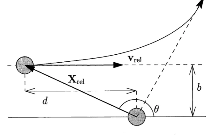
Here, we will be mainly interested in the chemical reactions and other dynamics which take place in bimolecular collisions. The application of classical mechanics to the simulation of bimolecular collisions is well known [21], and only the minimum of relevant details will be reprised here. The initial positions and velocities of the atoms in the colliding molecules are partially determined. We will assume that the reactant molecules are far apart before the collision (say at t = 0) and are moving towards each other. This basic scenario is illustrated in Fig. 2.1.
[image:41.531.100.443.354.575.2]2.1 R e a c tio n D y n a m ics 18
The relative motion of the reactants can be viewed as initially taking place in a plane formed by the relative position vector, X rei, that connects their centers of mass, and the relative velocity vector, v rei, as shown in the figure. The impact pa rameter, 6, measures the separation of the reactant centers of mass, perpendicular to the relative velocity vector. If the reactants did not interact with one another, then b would be the closest distance between the molecules (realised as they pass one another). The initial relative translational energy for the collision is Ere\:
where /i is the reduced mass of the pair. The angular momentum for the collision in Fig.2.1 is L (the orbital angular momentum):
In the gas phase, each reactant molecule experiences collisions with other molecules in three dimensional space (not a single plane) so that the number of collisions that have an impact parameter of value b is proportional to the circum ference of an anulus of radius 6, that is 2nb. After the collision has taken place, the molecules fly apart and at infinite separation, the angle, reaches a constant value called the scattering angle.
In order to simulate a molecular collision in the gas phase, we must take account of the fact that there are many different collisions, because there are many different values of the initial positions and velocities of the atoms which are consistent with Fig. 2.1. Clearly, the orientation of the molecules at t = 0 is arbitrary. The molecules may be rotating, so the rotational motion must be specified. In this work, for convenience, we generally assume that the reactants are not rotating. The reactant molecules are vibrating before the collision, so the energies of the vibrational motions and the phases of the vibrational motions must be specified.
-S'rel 2 ^ i ^ rell » (2.15)
2.1 R e a c tio n D y n a m ics 19
The selection of these initial conditions, vibrational phases, orientation angles, impact parameters, etc is achieved by a random sampling process that is called Monte Carlo sampling [21]. The details are not important here, we simply use
mented previously. [2]. A classical simulation of a chemical reaction is therefore a set of hundreds or thousands of classical trajectories each of which has initial atomic positions and momenta, chosen by Monte Carlo sampling, consistent with a bimolecular collision. The outcome of such a simulation is a random (Monte Carlo) sample of the bimolecular event. The measures we obtain of this process are statistical measures of averages. For example, by simply counting how many trajectories have molecular fragments of different composition than obtained at t = 0, we can calculate the probability of reaction. To be more quantitative, we calculate the reaction cross-section, a:
where P(b)db is the probability that collisions which had an impact parameter between b and b + db will lead to reaction. Since our classical trajectories conserve the energy of the molecule, the reaction cross-section describes reaction at a specific energy, cr(E). This cross-section is related to the thermal rate coefficient for the reaction by a thermal average [22]:
standard techniques to simulate bimolecular collisions, as described and imple
(2.17)
2.2 In ter p o la tio n o f P o te n tia l E n erg y S urfaces 20
Thus, one outcome of a classical simulation of a chemical reaction is the pre diction of a thermal rate coefficient. However, in order to calculate important quantities like rate coefficients, we must have a PES, that is, a knowledge of how the total electronic energy depends on the shape of the molecule at every molecular configuration required in Eq. (2.13). The basic approach used to achieve this is via interpolation of ab initio quantum chemistry calculations of V (R ).
2.2 Interpolation of Potential Energy Surfaces
Since the computational cost of evaluating V (R) by ab initio methods is very high, the number of molecular configurations at which V(R) is calculated will be small. In order to approximate V( R) elsewhere, we will use an interpolation method.
For reactions involving only three atoms, a number of interpolation methods have been reported [23-25]. However, in this work, we are concerned with the development of methods which can be applied to large molecules. The only sys tematic and efficient interpolation method yet reported for reacting molecules of more than three atoms is the Shepard interpolation approach introduced by Collins and coworkers [1-13].
2.2.1
Shepard Interpolation
2.2 In ter p o la tio n o f P o te n tia l E n erg y S urfaces 21
possible then to approximate the PES in the vicinity of that geometry by a second order Taylor series. To ensure that this approximation to the PES is invariant to translation and rotation of the molecule, the Taylor series must be expressed in internal coordinates. As suggested earlier, the atom-atom distances provide a con venient basis for internal coordinates. Actually, it is more appropriate on physical grounds to use the reciprocal distances,
Za = ^ ~ , i , j = l , . . . , N \ a = l , . . . l)/2 . (2.19)
Thompson, Jordan and Collins [7] showed how to construct 3N — 6 independent internal coordinates as linear combinations of the Za :
N ( N - 1)/2
Pk= Y Uk° Z°' k = 1 , 3 N - 6. (2.20)
a = l
The energy derivatives with respect to Cartesian coordinates can then be trans formed into derivatives with respect to these internal coordinates to write a Taylor expansion about some “data point” , Z(i):
3 N —6
dV
Ti(Z) = V [Z(i)] + Y\P* - ä WI k=1
3 N —6 3 N —6
p=p{i)
+ if
Y
E
_
- «(*)]
k=1 l—l
d2V
dpk dpi p = p (0 + .. (2.21)
If we have such Taylor expansions for i = 1, . . . , Nd data points, then we can write the PES as a weighted average or Shepard interpolation [26, 27]:
Nd
V(Z) = Y Y ^ W
T*°M-g&G i= l
2.2 In ter p o la tio n o f P o te n tia l E n e rg y S u rfaces 22
The rather compact notation in Eq. 2.22 requires some explanation. First, the symbol G stands for the symmetry group of the molecule; the Complete Nuclear Permutation Inversion (CNPI) group. Permutation of the coordinates of indistin guishable nuclei in the molecule does not change the energy and simply permutes the atomic labels on the energy derivatives. Hence, if we evaluate the coefficients in the Taylor series of Eq. (2.21) at some Z(z), we can easily form a Taylor series expansion about any permuted point, go Z(i). Thus, the sum over g in Eq. (2.21) implies that all symmetry equivalent versions of one data point are included in the data set. This ensures that the PES has the correct symmetry (and provides data points “for free”). The normalised weight function in Eq. (2.21) is given by
w i (Z) = V i ( Z )
^ 2 g E G Y l k= 1V9 ° k (Z)
where the unnormalised weight function v is
(2.23)
1
liz-zwii2”’
using the greater value of p > 3 N —6 or p > riTayior where riTayior is the degree of the Taylor polynomial1. Second order Taylor expansions are typically favoured, since higher order derivatives are expensive to calculate and are not such a significant boon as to make the effort worthwhile [4].
For appropriate weight functions, including that in Eq. (2.24), the interpolation formula of Eq. (2.22) becomes exact in the limit of high data density. Hence, convergence of the PES to the exact value should be observed as the size of the data set increases.
In actual fact there is usually only a small fraction of the data set which signif icantly influences the potential in any particular region of the PES. To reduce the
2.2 Interpolation o f P otential Energy Surfaces 23
num ber of com putations to a necessary minimum, the concept of a neighbour list
may be invoked, a concept from m olecular dynam ics [2, 28]. The requisite assum p
tion is th a t normalised weights below a given tolerance, wto\ are not included in the
neighbour list and are therefore not used to calculate th e interpolated potential in
Eq. (2.22).
In a trajecto ry calculation, every fixed num ber of tim esteps the neighbour list
is u p d ated to ensure th a t the correct neighbours in the new region of configuration
space are used. This u p d ate is perform ed only often enough to keep th e introduced
discontinuities small b u t still reduce the com putation tim e. Hence, the aim should
be to keep th e tolerance, iutoi, small enough th a t th e identity of th e neighbours
changes slowly. An extension of this idea is to use inner and outer neighbour lists,
where one list is up d ated less frequently b u t contains a larger list of points. The
outer neighbour list is larger because it includes d a ta points whose weight exceeds
Wtoi,o, where iutoi,0 <
1-O ther functional forms have been tried for th e unnorm alised weight function [7].
A two-part unnorm alised weight function has been suggested for larger system s
such as CH4 + H [7]:
Vi (Z) Z - Z(i)
rad (i)
2v
+ Z - Z (i)
rad(i) 2q
(2.25)
which is consistent w ith the asym ptotic lim its of th e former, one-part formula,
where p and q are adjustable param eters. A form of the tw o-part weight function
has recently been introduced using inform ation ab o u t the accuracy of the Taylor
expansions to modify the function [8, 9], which will be discussed later in this
chapter as it has become th e m ethod of choice, and has been used tow ards the end
2.3 S am p lin g Im p o rta n t R e g io n s o f th e P E S 24
2.3
Sam pling Im portant R egions o f th e PES
The interpolation formula Eq. (2.22) should converge to the exact result as the size of the data set increases. However, we cannot just calculate a series of ab initio data points to produce a reasonably continuous data set that can be accurately interpolated because of computational feasibility. If some number of data points, M, was required for a dense set (or grid) of data in one dimension, then a dense set in 37V —6 dimensions would require M3N~6 data points. This is an impossibly large number of ab initio computations for TV > 3. Also, one must be aware that as the number of atoms in a system is increased (worse if these have many electrons, or are so-called “heavy atoms”), the complexity of these calculations increases rapidly with this increased dimensionality. Hence, we would prefer to obtain an accurate surface by interpolation using as few ab initio points as possible, particularly in systems larger than triatomics.
2.3 S am p lin g Im p o rta n t R e g io n s o f th e P E S 25
2.3.1
Iterative Schem e
1. Choose a small set of data point geometries on intuitive, physical, grounds. For example, configurations that lie on the minimum energy path (MEP) for some reaction of interest. There are standard methods in ab initio quantum chemistry programs for finding such paths. The PES from Eq. (2.22) is now dehned with this data set.
2. Evaluate classical trajectories to simulate the bimolecular collision using the interpolated PES with the current data set.
3. Molecular configurations are sampled from this batch of trajectories. The number of trajectories can be small, but large enough to represent the relative im portance of different regions of configuration space for different reaction channels. 4. Choose a trajectory configuration from this sample to be a new data point. The choice is made using criteria described below. The basic idea is to choose configurations that are most likely to improve the accuracy of the interpolated PES.
5. Perform the necessary ab initio calculations and add this point to the data set. 6. Repeat this process from step (2) until the PES is “converged.”
2.3.2
Selection Criteria
In step (4), we have to choose which (of thousands) of molecular configurations will be a new data point.