Energy saving in a 5G separation architecture under different power model assumptions

power model assumptions

.

White Rose Research Online URL for this paper:

http://eprints.whiterose.ac.uk/111401/

Version: Accepted Version

Article:

Fisusi, Abimbola Adeola, Grace, David orcid.org/0000-0003-4493-7498 and Mitchell, Paul

Daniel orcid.org/0000-0003-0714-2581 (2017) Energy saving in a 5G separation

architecture under different power model assumptions. Computer Communications. pp.

89-104. ISSN 0140-3664

https://doi.org/10.1016/j.comcom.2017.01.010

[email protected] https://eprints.whiterose.ac.uk/

Reuse

This article is distributed under the terms of the Creative Commons Attribution-NonCommercial-NoDerivs (CC BY-NC-ND) licence. This licence only allows you to download this work and share it with others as long as you credit the authors, but you can’t change the article in any way or use it commercially. More

information and the full terms of the licence here: https://creativecommons.org/licenses/

Takedown

If you consider content in White Rose Research Online to be in breach of UK law, please notify us by

Energy Saving in a 5G Separation Architecture under Different Power

Model Assumptions

Abimbola Fisusi*, David Grace, Paul Mitchell

Communications and Signal Processing Research Group, Department of Electronics, University of York, York, YO10 5DD, United Kingdom

ABSTRACT

In this paper, a framework is developed to study the impact of different power model assumptions on energy saving in a 5G separation architecture comprising high power Base Stations (BSs) responsible for coverage, and low power, small cell BSs handling data transmission. Starting with a linear power model function, the achievable energy saving are derived over short timescales by operating small cell BSs in low power states rather than higher power states (termed Low Power State Saving (LPSS) gains) for single and multiple BS scenarios. It is shown how energy saving varies with different power model assumptions over long timescales in accordance with short timescale LPSS. Simulation results show that energy saving in the separation architecture varies across the six power models examined as a function of model-specific significant LPSS state changes. Furthermore, it is shown that if the architecture is based on existing small cell BSs modelled by state-of-the-art (SotA) power models, energy saving will be mainly dependent on sleep state operation. Whereas, if it is based on future BSs modelled by visionary power models, both sleep and idle state operations provide energy saving gains. Moreover, with future BSs, energy saving of up to 42% is achievable when idle state overhead is considered, while a higher saving is possible otherwise.

Key Words: Separation architecture, energy saving, power models, low power state saving, 5G

_______________________________________________________________________________________________________

1. Introduction

Several fifth generation (5G) mobile systems proposals, such as [1] and [2], have identified Energy Efficiency (EE) as an important requirement in 5G systems. This is due to concerns about the economic and environmental consequences of providing 5G services using existing network paradigms mainly focussed on maximizing capacity by increasing transmit power [3]. Already, significant increase in energy consumption of cellular networks has been linked to the large number of smart phones and tablets accessing mobile data and video applications via 3G and 4G networks [4]. Furthermore, increasing demand for mobile data and video traffic has necessitated deployment of more and more Base Stations (BSs) [4, 5]. Further increase in energy consumption is the outcome; this is because BSs account for over 50% of the total power consumption of existing cellular networks [6]. Future 5G systems are expected to support Machine to Machine (M2M) communication which could involve billions of machines [7]. It is also believed that 5G systems will support 1000 times the system capacity of 4G systems [8]. However, providing the desired 1000x capacity by simply scaling transmit powers will result in unacceptable high cost of operation [3] and emission of greenhouse gases beyond acceptable levels [9]. In contrast, the 1000x capacity is required to be provide at energy consumption levels similar to those of current cellular networks [9]. Hence, EE is even more critical for 5G.

In order to address the critical challenge of EE in 5G systems, the concept of separation of the data and control (or signalling) planes has been proposed, with high power ______________

*Corresponding Author

Email Addresses: [email protected] (A. Fisusi), [email protected] (D. Grace), [email protected] (P. Mitchell)

macro BSs handling the control functions while low power small cell BSs serve user data only [1, 10]. This approach enables coverage of the service area to be provided by the high power BSs while the capacity needs are met by the low power BSs. As a result, at low traffic loads most of the low power BSs can be switched off without compromising the network coverage requirement. In addition to handling coverage, the macro BSs can be configured to handle low-data rate user requests, while small cell BSs handle high-data rate requests [11, 12]. This type of architecture has been described as a Hyper-cellular network in [13] and referred to as a Separation Architecture in [11]. This architecture can significantly reduce signalling overhead in the small cell layer, optimise the resource utilisation and improve energy efficiency [13]. The energy saving in such an architecture is the focus of this study.

Whereas [12] and [14] do not seek consistency with existing standards, in [11] a signalling approach suitable for existing wireless standards is considered. As a result, in [11] the small cell data BSs still carry a reduced set of overhead signals including pilot (or reference) signals. However, coverage and low-rate data services are still handled by macro control BSs while data BSs handle high-rate data services. In [15], based on the separation architecture paradigm, a conventional macro BS is replaced with a low power coverage BS (CBS) and several small cell traffic BS (TBS). While the CBS handles coverage, the TBS handles data services. Based on a SotA 2010 model, power consumption is estimated for fixed (TBS always on) and dynamic (TBS on/off) configuration. The separation architecture achieves significant savings (50% or more) over the conventional macro BS approach.

In [16] a separation architecture is proposed for future 5G cellular systems with small cell BSs operated at higher frequencies like 3.5 GHz while the Macro BSs utilise conventional lower frequencies of 2 GHz similar to LTE. Nearly 75% percent energy efficiency gain is achieved since unlike in LTE most small cell BSs can go into deep sleep while macro BSs guarantee coverage. In [17] the joint optimization of density of BSs, number of antennas and spectrum allocation for energy efficiency in a separation architecture based HetNet of macro BSs and small cell BSs is investigated. The combination of small cell BSs and multiple antennas is shown to provide significant energy saving relative to a single antenna macro BSs only system.

The optimal resource partition among signalling and data BSs is studied in [18] while a probabilistic sleep mechanism is designed for the data BS layer of a separation architecture in [19]. In [20] the trade-off between total energy consumption and overall delay for a Data BS of a separation architecture is studied while the ratio of small cell BSs, that can be put to sleep as the traffic load varies, is investigated in [21]. In [22], energy saving is investigated in a separation architecture where the small cells in sleep modes are activated with the help of a macro BS and user association to a small cell is also carried out by the macro BS.

Resource allocation strategies are developed in [23] for a phantom cell based separation architecture to either optimize energy efficiency or optimize spectral efficiency. In [24] on-grid power saving is studied in a separation architecture where small cell BSs can be powered by grid and/or renewable energy sources and are used to offload traffic from macro BSs. In [25] throughput and EE performance is studied in a separation architecture with files cached at the BSs and limited backhaul infrastructure. Furthermore, in [26] sleeping strategies are proposed for a separation architecture in which small cell BSs form co-operative clusters to provide high data services. Also in [27] the effect of BS sleeping on the EE of a small cell BS belonging to separation architecture and the user-perceived delay is studied and optimal energy saving policies are designed under the constraint of mean delay for different wake up schemes. In addition, in [28] an energy saving

framework based on feedback information from user equipments is developed for a separation architecture where small cells are user or operator deployed. In [29] a BS sleeping scheme is proposed to put data BSs of a separation architecture into one of two sleeping stages depending on the presence of users in their coverage area.

Furthermore, future evolution of the LTE/LTE-A standard would be able to support separation architectures through the “dual connectivity concept” [30]. Dual connectivity permits user equipment (UE) to be served simultaneously with radio resources from two BSs. Energy saving under the consideration of different backhaul technologies in a separation architecture based on the LTE-A Dual Connectivity is investigated in [31]. In [32] an energy efficient algorithm with consideration of secrecy is proposed for uplink traffic offload in a dual connectivity network with small cell operated in unlicensed band.

Although, the energy savings of separation architectures have been studied under different implementation regimes (as discussed above), the impact of the choice of power model (which depends on the BS generation) on energy saving of a separation architecture has not been studied in the literature to the best of our knowledge. This sort of study is important because it can facilitate an understanding of how energy saving varies with respect to power model assumptions. This knowledge can aid the design of suitable energy efficient resource and topology management strategies or the enhancement of existing strategies.

In this paper, we consider simplified linear power models derived from the initial proposal of the EARTH project [33, 34], which demonstrates that the power consumption of a BS varies linearly with the transmitted power. In addition, we focus on high level aspects of the power models, in this case the variation in the power consumption of a BS in different operating states with different power model assumptions. This variation is due to different BS hardware enhancements expected in the future and suggested in the literature [35-37] and herein. Furthermore, we explore the possibility of the BS power consumption in the idle state approaching the consumption in the sleep state and the power saving when operating small cell BSs in a sleep state and an idle state. Also, we consider a light sleep state only under which few BS components are deactivated and the BS can be quickly reactivated in about 30 µs while the BS enters into a sleep state instantaneously [35].

This is in contrast to the proposal in [38], where detailed BS hardware components’ power consumption are considered in the design of a flexible power model suitable for BSs of different types for the period 2010 to 2020. Also in [38], the energy saving potentials of different levels of sleep states is the focus rather than both sleep and idle states and comparison is done for single BS cases rather than in a network of BSs.

 Is there significant benefit with regard to energy saving in operating small cell BSs in idle state and sleep state for each power model?

 How do different BS state transitions affect the energy saving for each power model?

 How does the energy saving of these models compare with one another?

We address these questions by developing a framework aimed at evaluating the power saving achievable when BSs are operated in lower power consumption states rather than high power consumption states (termed Low Power State Saving (LPSS)). The framework includes generic equations derived for estimating LPSS over very short timescales for both single and multiple BS scenarios. The short timescale LPSS provide the basis for understanding energy saving over long timescales. Furthermore, a miniature separation architecture model comprising a high power BS and four small cell BSs is also included in the framework to swiftly identify the BS state changes in the small cell layer that contribute significantly to energy savings for each power model. Finally, system level simulation is included to evaluate energy saving and QoS performance of an energy efficient resource management scheme under consideration of the different power models in the full scale architecture.

The remaining section of the paper is organized as follows. In section 2, the system model is presented, while the LPSS framework is discussed in section 3. The simulation results are presented and discussed in section 4. Finally, the paper is concluded in section 5.

2. System Model

2.1. Network Architecture

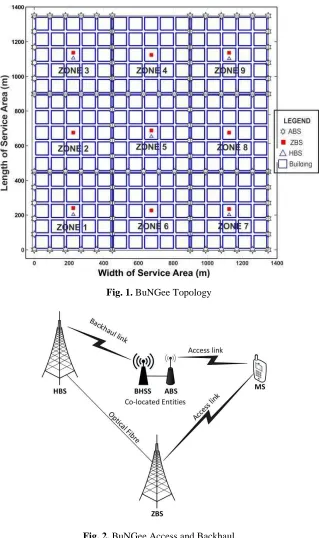
The access network of the Beyond Next Generation mobile broadband network (BuNGee), which has been modified in this work to include high power control BSs in each zone (referred to as Zone Base Station (ZBS)), is considered. BuNGee is a cost-effective, mobile broadband architecture with the goal of a high capacity density of at least 1Gbps/km2 studied under the FP7 BuNGee Research project [39]. The BuNGee Architecture is based on a two-tier deployment of access and backhaul network [40]. The access network consists of the BSs that provide resources used to serve user requests while the backhaul network connects the access network to the core network. The BuNGee access network consists of a dense deployment of small cell BSs, referred to as ABSs, in a regular pattern as shown in Fig. 1. The ABSs are low cost, low power, simple, below rooftop BSs. The ZBSs are the control BSs and have been introduced in the access network to facilitate the separation of the control and data plane.

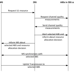
The backhaul network consists of Hub Base Stations (HBSs) and Backhaul Subscriber Stations (BHSSs). The BHSSs are co-located with the ABSs, so at each ABS location there is a complementary BHSS for backhauling Mobile Station (MS) information to a HBS as shown in Fig. 2. The HBSs are high power, wide coverage base

stations deployed solely for backhauling. They serve as high capacity hubs for the network through 24-beam, dual-polarized antennas at 3.5GHz [40]. Backhauling is achieved through in-band and millimetre Wave (mmWave) transmissions. The in-band backhauling involves the link between a BHSS and an HBS while the mmWave backhauling involves shorter link distances between BHSSs, due to the shorter range of mmWaves. It is assumed that separate frequency bands are used for the access and backhaul network and interference between the two tiers is completely avoided. Low latency, high capacity and reliable backhaul is provided between the HBSs and BHSSs through the combination of the in-band and mmWave backhauling as demonstrated in [41].

The ABSs are deployed outdoors along the streets in the service area. Each ABS is equipped with two directional antennas which point in opposite directions. One antenna points up the street, the other points down the street. Two ABSs are co-located at the intersection of two streets. The fixed frequency plan [42] specified in the BuNGee project is used here. According to this plan, the two antennas of an ABS operate in different frequency bands. Four directions are considered - North, South, East and West - and an ABS can have North and South pointing antenna beams or East and West pointing antenna beams. In order to mitigate interference, the antennas of adjacent ABSs facing the same direction operate in different frequency bands and two antennas belonging to different ABSs but pointing along the same street also operate in different frequency bands. Four unique frequency bands are assigned to the small cell layer and each frequency band has a bandwidth of 10 MHz. In this work, each frequency band is further divided into 10 unique subchannels and each subchannel on a particular ABS can be assigned to only one MS. Each MS is assigned only one subchannel at a time for uplink transmission.

The MSs are distributed uniformly outdoors in the service area and each MS is equipped with an omnidirectional antenna with a gain of 0 dBi. The service area is divided into nine square zones as shown in Fig. 1 and ABSs can be associated with up to a maximum of four zones. ABSs can only communicate directly with their adjacent neighbours while they can communicate with the ZBSs through backhaul links. The ZBSs share a 10 MHz frequency band that is out of band to the ABS bands.

Fig. 1. BuNGee Topology

Fig. 2. BuNGee Access and Backhaul

As shown in Fig. 2, each ZBS is connected to a nearby HBS through optical fibre and information exchange is possible with low delay between a ZBS and an ABS through the backhaul links between a HBS and a BHSS. mmWave links between BHSSs may also be utilized for diversity in case of failure of the direct link between HBS and a particular BHSS. Whenever an MS has to be served in the DL or UL, the serving ZBS requests the ABSs in its

Request UL resource

Request channel quality measurements

Send channel quality measurements

Inform MS about selected ABS and resource

allocation decision

MS synchronizes with selected ABS

Uplink Transmission to selected ABS

MS ZBS ABSs in ZBS zone

Alert selected ABS and inform about resource allocation decision

Fig. 3. Co-ordination Procedure for UL Data Transmission

The channel between an ABS and a MS is modelled using the WINNER II B1 propagation model for Urban Micro-cells [44] since the ABSs and MSs are deployed outdoors. The transmission rate per bandwidth, R, over the channel is determined from the Truncated Shannon Bound (TSB) [45] as follows:

=

0 ; < log21 + ; < <

max ; >

(1)

is the attenuation factor, SINRmin is the minimum SINR

required for reception, SINRmax is the SINR at which the

maximum throughput, Rmax can be achieved. The

parameters of the BuNGee-specific TSB [42] are = 0.65, SINRmin = 1.8dB, SINRmax = 21dB and Rmax = 4.5bps/Hz.

2.2. Power Consumption and Energy Saving

The power consumption of the access network is estimated to be 80% of the entire wireless network consumption and the base stations are mainly responsible for this huge share of the access network [46]. Therefore, the energy saving at the BSs is the focus in this work. In particular, we consider the energy savings that can be achieved in the access network by switching some of the ABSs into low power consumption states when uplink data transmissions from MSs are being served. The power consumption of the backhaul network including the HBSs and BHSSs are not considered but the backhaul network have been explained earlier to show how information exchanges between ZBSs and ABSs in the access network can be implemented practically.

In existing wireless systems, unlike in macro BSs where the load dependent power amplifier (PA)

consumption is dominant (55-60%), for low power BSs (i.e. micro, pico, and femto BSs) the PA share of the power consumption is much smaller (less than 30%) in currently deployed systems [34]. Hence, power consumption of micro BSs are much less load dependent than macro BSs while power consumption of pico and femto BSs hardly scale with load [33]. As a result, the full load downlink power consumption of small cell BSs is of similar order of magnitude as the uplink and no load conditions in existing systems. Hence, it is important to consider the energy savings at BSs in the uplink for a network with an ultra-dense deployment of small cells.

3. Framework for LPSS Evaluation

Generally, a BS can operate in active, idle, or sleep states. In the active state, it receives and/or transmits data, whereas in the idle state it is powered on but waiting to serve user requests. When traffic levels permit, a BS can be operated in the sleep state where it consumes lower power than in the active or idle states, but cannot serve user requests. A BS can achieve some power saving when it operates in a low power state rather than a higher one. The power saving due to BSs operating in low power states rather than higher states (termed Low Power State Saving (LPSS)) under different power model assumptions is examined for uplink transmission.

since file transmissions take significantly longer time compared to the reactivation time of about 30 µs.

3.1. Power Models

Power models are usually required to estimate the total power consumption of a BS. These models usually comprise a static part and a dynamic part. The static part is independent of the traffic load and output transmission power. It instead includes losses in the power supply, signal processing, and cooling systems [47]. On the other hand, the dynamic part is dependent on the traffic load supported by the BS and thus a function of the output transmission power. The power consumption of any type of BS can be approximated by a linear function [33, 34] as follows:

= 0+ . , 0 <

. , = 0 (2)

is the BS total power consumption, is the output transmission power, is the maximum transmission power, 0 is the no load power consumption

measured at the lowest possible non-zero output power, is the number of transceiver chains, while is the slope of the load dependent dynamic consumption part. is the power consumption when the BS is switched to sleep state. The sleep state consumption, , is lower than the no load consumption, 0, because it is assumed

that in the sleep state, some BS components can be deactivated to further reduce power consumption [48].

Even in the idle state, when no user data is transmitted by a BS, between 10% and 20% of the maximum transmission power is used to transmit reference and control signals (which constitutes overhead) in state-of-the-art (SotA) cellular systems (e.g. LTE) [49]. Hence, the instantaneous output transmission power, , is a combination of the power needed for signalling and power for user data. According to [50] for SotA cellular systems, the instantaneous output transmission power is given by:

= 1 + (3)

is the fraction of the transmit power required for fixed overhead signals (0 < 1), is the fraction of the total bandwidth used for data transmission, and is a weighting factor that indicates the level of overhead transmitted depending on the state of the BS (0 1). The value of for different states are as follows [50]:

=

0 0.5 1

(4)

In the sleep state, both overheads and user data are not transmitted, partial overheads are transmitted in the idle state, while the complete set of overheads is transmitted in the active state. is assumed to be 0.2 herein, since as

stated earlier, up to 20% of the maximum transmission power may be used to transmit overheads [49].

For uplink transmission, BS transmit power is expended on overhead only since no user data is transmitted by the BS. Hence, = 0 and the output transmit power, , is as follows for the uplink case only:

= (5) As stated earlier, up to 50% reduction in overhead signal transmission relative to 4G systems utilizing CRS is possible at the small cell BSs through the separation architecture [43]. Hence, from (4) overhead weighting factor under the separation architecture, , equivalent to 50% overhead reduction is adopted herein for each BS state as follows:

=

0 0.25 0.5

(6)

While the energy consumption of the small cell BSs can vary with the operating state, the energy consumption of the ZBSs is assumed constant since the ZBSs are always on and can be considered to always be in the idle state since the case of data transmission by the small cell BSs alone is considered herein.

The linear function in (2) can be expressed in terms of static and dynamic parts and with the incorporation of the three possible BS states as follows:

= + . , 0 (7)

= . 0,

. , (8) = . ,

0 , (9)

is considered to be the static power consumption. This is because ₀ is a parameter that represents BS power consumption at zero output but which is usually measured at 1% of the maximum output transmit power [51]; also measures power consumption at zero output but with some BS components deactivated. is considered as the dynamic part since the output transmit power varies with the load. The variation could be due to reduction in occupied subcarriers and/or subframes [33].

_

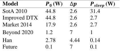
= . + (10) _ _{and are dBm power values, while a and b are} constants: a = 0.618 and b = 26.1. From (10) the maximum power consumption of each 2x2.5W ABS is 102.6W. Other relevant power model parameters of the ABSs can be obtained from (2).

Six power models ranging from a state-of-art 2010 (SotA 2010) model to a future model are considered. Four of the models – SotA 2010, Improved DTX, Market 2014 and Future Models – were previously considered in [37] for a single macrocell scenario. The Han model proposed in [52] and Beyond 2020 model (proposed in this study) complete the set of power models. The ABS specific linear model parameters for the different models are provided in Table 1 for a single transceiver chain.

Table 1

Linear Model Parameters for Different Power Models

Model (W) (W)

SotA 2010 44.8 2.6 31.4

Improved DTX 44.8 2.6 2.7 Market 2014 17.9 2.6 2.7

Beyond 2020 1.2 7 1

Han 2.78 4.44 0.14

Future 0.1 7 0.1

The SotA 2010 model is based on the linear power modelling of SotA BS types in 2010 proposed in [34]. The SotA 2010 model is specified for a 2x6.3W microcell in [34]. The parameters for the 2x2.5W ABS considered herein are obtained using (2) as follows. Assuming the same slope, = 2.6, as in [34] and with the maximum power consumption and maximum transmission power (102.6W and 2.5W per transceiver chain respectively) already known, the no load consumption, ₀, can be determined from (2). The sleep state consumption, , is obtained from the ratio between the sleep and no load consumption in [34].

The improved DTX model proposed in [35] assumes that significant power consumption reduction can be achieved through cell DTX, which is a procedure that switches the BS to sleep state. This is because sleep state consumption is only approximately 6% of the no load consumption. However, the no load consumption is unchanged since enhancement of BS hardware is not considered in this model. The Market 2014 model (so called in [37]) suggested in [36] assumes that in addition to the sleep mode capability, BSs are designed with more power efficient components in the future. Hence, a substantial reduction in no load consumption (approximately 40%) is assumed in addition to the sleep mode saving.

A beyond 2020 model is also proposed to reflect the expected design of BSs to have nearly perfect load dependency and very low sleep and no load power

consumption. Hence, a sleep mode consumption that is much lower than the 2014 status is assumed. In addition, rather than a 100 percent increase in power from the sleep to no load consumption assumed for a 2020 small cell model in [53], a much lower increase of 20% is assumed in this case. This model is used to explore the impact of idle state consumption (a function of the no load consumption) approaching the sleep state consumption. The Han model, proposed in [52], assumes a relatively low no load power consumption and nearly zero sleep mode consumption. In addition, it accounts for power consumed in reactivating a BS in sleep state. However, the contribution of reactivation energy has been observed to be trivial and it is not considered in the linear adaptation of this model. The extra power cost incurred by signalling is not accounted for in all states and ABSs transmit at maximum power when active under this model.

Finally, the Future model proposed in [37] provides a theoretical limit for power consumption. This model results in a near perfect load-dependent power consumption; also, the no load consumption is exactly the same as the sleep state consumption. It is assumed here that no extra power cost is incurred for overhead ( = 0) in the idle state. This is possible with overhead transmission completely disabled in the idle state. However, overhead power is included in the active state (uplink/downlink). Hence, power is mainly utilized when users are being served.

3.2. Short Timescale LPSS in Single BS Scenario

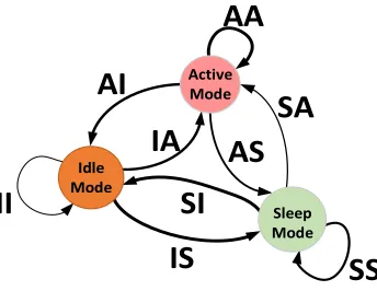
An ABS can be in any of the three possible states at a given time and may make the transition to a different state after a period of time (as shown in Fig. 4). In the same vein, an ABS may operate in a particular state under a certain resource management scheme but operate in a different state under another scheme for a similar observation period and system settings. When the ABS is monitored over a very short timescale of the order of magnitude of the time between user arrivals or departures (few milliseconds to seconds), it is possible to observe single state changes. Over longer timescales (a couple of minutes or hours), the ABS may undergo several state changes. We first focus on the short timescale and develop the LPSS concept. Subsequently, LPSS over the long timescale is considered.

If an ABS changes state under the control of a resource management scheme from an initial state in which its power consumption is ₁ to a new state where it consumes

2 and remains in this new state for a time period, t; some power saving (LPSS) will be achieved as a result of this state change for the considered period, t, if ₁> ₂. Similarly, if an ABS is monitored over a fixed period of time and fixed system setting (e.g. fixed traffic load and distribution) under two different resource management schemes, one scheme can achieve power saving relative to the other if the ABS effectively operates in different states under the different schemes. The equations derived subsequently are applicable to both the state change and the state difference cases and both are used interchangeable.

II

IS

IA

AA

AI

SS

SA

AS

SI

Active Mode

Idle Mode

Sleep Mode

Fig. 4. BS Possible State Changes

Whenever there is a state change, there is a potential increase or decrease in power consumption relative to the initial state. However, only the active to idle (AI), active to sleep (AS) and idle to sleep (IS) state changes lead to power saving. From (7), we can obtain a generic expression for the LPSS due to any of the state changes above. If the BS was initially in a state 1 and changes to a new state 2, the LPSS, ₁₂, can be expressed as follows:

12= ,1 ,2+ ( ,1 ,2) (11) ,1, and ,2 are the static power consumption in state 1 and state 2 respectively, while _,1 and _,2 are the dynamic power consumption in state 1 and state 2 respectively. is the slope of the dynamic part. The LPSS gain, _,12, which expresses the LPSS, ₁₂, as a ratio of the power consumption in the initial state, ₁ , can be defined as follows:

,12=

12

1 =

,1 ,2+ ( ,1 ,2)

,1+ . ,1

(12)

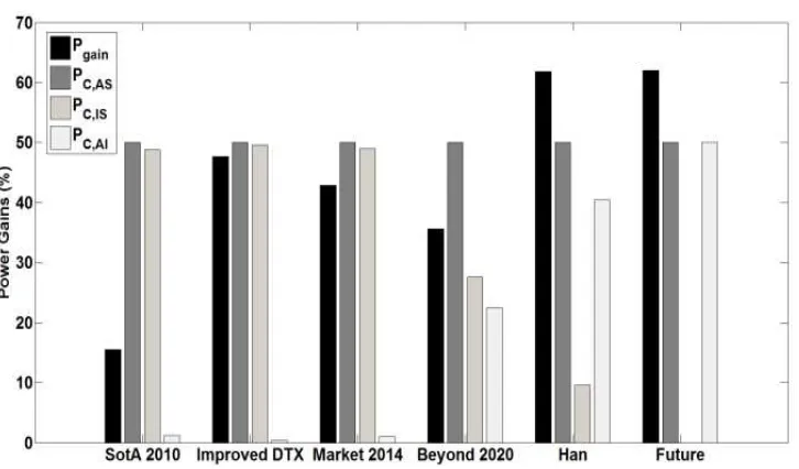
The LPSS gains for different state changes under different power model assumptions for a single BS are shown in Fig. 5. The uplink is considered in this study; thus, the active state represents the periods an ABS is receiving data transmission from MSs. It can be observed from Fig. 5 that the significant state changes and the potential for power saving varies from model to model. The SotA 2010 model shows the lowest potential for power saving because it has comparatively high no load consumption and sleep mode consumption, resulting in a lower range of power saving. Other models show better potential for power saving because of significantly lower sleep state consumption and in some cases low static consumption. The SotA 2010, Improved DTX and Market 2014 show almost no benefit for operating the ABS in an idle state. On the other hand, the remaining models, show appreciable power savings when an ABS is operated in an idle state instead of an active state. It is important to note that power saving is still possible for the idle state to the sleep state transition even when the no load consumption,

0, is almost equal to sleep mode consumption, , because of the extra power incurred in the idle state for overhead signals in non-ideal models as in the case of Beyond 2020 model. The Future model, which is an ideal model, alone does not benefit from switching idle BS to sleep state since consumption is the same in both states.

3.3. Short Timescale LPSS in Multiple BS Scenarios

The LPSS concept is also extended to multiple BS scenarios comprising several BSs. This is typical of the small cell layer of the separation architecture. In this case, the LPSS gains are expressed in terms of the relative importance of the different state changes on a global scale (i.e. multiple state changes and multiple BSs). The equations are derived based on state differences and assumption of different resource management schemes. It is assumed that the first scheme is a baseline resource management scheme that requires all ABSs to always be on (i.e. either in active or idle state). This is similar to conventional always-on resource management schemes with the goal of spectral efficiency rather than energy efficiency. The second (test) scheme is an energy efficiency driven scheme and can switch off (or switch to the sleep state) BSs under favourable conditions. With the baseline scheme as the reference scheme, the LPSS gains can be evaluated for the test scheme.

The total power consumption of the baseline and test schemes are and respectively and expressed as follows:

= =1 , , + . , , (13)

= _{=1 , ,} + . _{, ,} (14) refers to the total number of BS, represents a BS state under consideration of the baseline scheme while similarly represents a BS state under consideration of the test scheme. Therefore, _{, ,} and _{, ,} are the static and dynamic power consumption of the BS in state with consideration of the baseline scheme. Similarly, _{, ,} and

Fig.5. LPSS Gains for Single BS

Therefore, following from (13) and (14), the total power saving of the test scheme with respect to the baseline scheme, is as follows:

=

= =1 , , + . , , =1 , , + . , , (15)

Two types of LPSS gain is defined for the multiple BS case: absolute and comparative. On one hand, the absolute LPSS gain, , , measures the actual saving due to a particular state difference between the test and baseline scheme for the period of observation with respect to the baseline power consumption. On the other hand, the comparative LPSS gain, _, , measures the saving of a particular state difference with respect to the total saving. Thus, the comparative LPSS gain shows explicitly the share of a particular state difference combination in the total saving whereas the absolute LPSS gain just shows its actual value. If is a LPSS of a single BS (kth BS) as defined in (11), then the absolute LPSS gain, _, , and comparative LPSS gain, _, , can be expressed as follows:

= , , , , + ( , , , , ) (16)

, = =

, , , ,+ ( , , , ,)

, ,+ . , ,

=1 =1 , ,+ . , ,

(17)

, = =

, , , , + ( , , , , )

, ,+ . , ,

=1

(18)

Hence, _, = _, × = _, × (19)

Where is the overall power saving gain of the test scheme relative to the baseline. Subsequently, comparative LPSS gain is evaluated over a snapshot of the BuNGee network using two resource management schemes previously proposed for the BuNGee Architecture as

baseline and test schemes. It is important to note that MS arrivals are modelled by flow level dynamics, which constitutes a random arrival of MSs into the network each with file transfer requests and departures from the network when files have been successfully transferred [38]. We consider the case where MSs send one file at a time and are assigned one subchannel for this purpose.

3.4. Resource Management Schemes

In some previous BuNGee evaluations [42, 52] the resource management strategy associates MSs with the closest ABSs that can offer them the highest uplink SINR. We refer to this scheme as the highest SINR scheme and use it as the baseline scheme. Under the control of this baseline scheme, the ABSs are never switched off (i.e. transition to a sleep state is not permitted).

The test scheme is a combination of a resource management scheme and a topology management scheme for multiuser resource assignment and ABS activation or deactivation respectively. The test resource management scheme is the Interference Aware Clustering Capability Rating (IACCR) scheme, which we proposed previously for the BuNGee architecture without plane separation [54]. The IACCR is an energy efficient centric scheme that also mitigates interference as well [54], while the topology management scheme is an enhancement of the one applied in our previous studies on BuNGee [54, 55].

3.5. Highest SINR Scheme

This scheme’s objective is to associate MSs with the

requests for the uplink SINR of the subchannels from the ABSs for the specific MS. However, only ABSs with uplink SINR subchannels higher than the call admission SINR threshold need respond. The ZBS will then instruct the MS to connect to the ABS with the highest SINR subchannel.

3.6. Interference Aware Clustering Capability Rating (IA-CCR) Scheme

Interference Aware Clustering Capability Rating (IA-CCR), proposed in [54], is an enhancement of the Normalized Clustering Capability Rating (NCCR), an energy efficient resource management scheme proposed in [55] for the BuNGee Architecture. NCCR is based on the principle of concentrating or clustering users around as few as possible ABSs, thus permitting a large number of ABSs to be switched off. The scheme prefers more central ABSs over those closer to the edge of the service area to serve MSs. This is because of the potential of the more central ABSs to cluster more users based on their location in the service area. The choice of ABS is based specifically on the computation of a clustering capability rating (CCR) value. The CCR value is a linear combination of two ABS location parameters and one ABS load parameter and it is evaluated as follows:

= + + (20) The location parameters are the zone association weight, Za, and location weight, Lw. The zone association weight,

Za, is the number of zones an ABS is associated with

normalized by the maximum possible zone association (which is 4). The location weight, Lw, is the reciprocal of

the normalized distance of an ABS to the centre of its zone. The ABS distance is normalized by the distance of the most central ABS to centre of the zone. The load parameter is referred to as the loading ratio, Lr, and it is the ratio of the

instantaneous traffic load on an ABS to the maximum traffic load it can support. These parameters have values between 0 and 1 due to the normalization in all cases. a, b, and c are constants, and a = 100, b = 10, and c = 1. These constants are used to achieve hierarchical scaling among the ABS parameters. The final NCCR value is obtained from the normalization of the CCR value by the maximum possible CCR value as follows:

= ; = 111 (21) An MS is served by an ABS with the highest NCCR value that meets the call admission SINR threshold.

At low traffic loads, the NCCR scheme can significantly reduce the number of active ABSs and provide opportunity for energy savings through deactivation of idle ABSs [55]. However, at medium and high traffic loads, it causes high interference in the network which in turn leads to both poor quality of service and low energy efficiency [55]. In [54], it is shown that the choice of ABS determines

the level of inter-cell interference among the small cell ABSs in the network. While, the highest SINR scheme which associates an MS with the closest and first choice ABS in terms of SINR results in low interference, the NCCR scheme permits MS association with any choice of ABS, which includes distant and higher order choices and thus results in very high interference.

The IACCR scheme mitigates the interference associated with the NCCR scheme whilst still achieving a good degree of clustering and energy saving. This is achieved by first applying a restriction policy that limits the ABS choice range for an MS before the final choice of ABS is made based on the NCCR value of the permitted choices. In this study, the choice of ABS to serve an MS is made by the ZBSs rather than the MS itself like in [54]. The IACCR scheme is implemented as follows: let Li and

Lmax represent the current traffic load and maximum

possible traffic load of an ABS i respectively; thus, the normalized traffic load, xi on ABS i at any instant can be

expressed as:

=

Let X = [xi] represent the vector of the normalized

traffic load of all ABSs in the zone, while S = [si] represent

the vector of the highest uplink channel SINR achieved at each of the ABSs. Let C = [ci] represent the NCCR vector

for the ABSs while sth represent call admission SINR

threshold. Given an nth choice restriction policy specified in the service area, which implies MSs are permitted to connect to the nth choice ABS or lower order (but better) choices, the final choice of ABS is determined as follows:

1. All elements of X, S and C are set to zero initially. 2. When MS requests for uplink resource, ZBS requests

channel quality measurement from ABSs in its zone. 3. Each ABS verifies the condition: si ≥ sth and sends si

to ZBS only if the condition is satisfied.

4. ZBS updates S with all received si, C with ci for each

ABS that responds, and then arranges the set of ABSs in descending order of SINR (si ). However, if no

ABS responds, the MS is blocked.

5. Assuming the total number of ABSs in the set is m, a ZBS will instruct the MS to connect to an ABS with highest ci value among the set of ABS, if m ≤ n.

However, if m > n ZBS selects the highest ranking n ABSs based on si, and instructs the MS to connect to

the ABS with highest ci value in the high ranking

ABS subset.

6. ZBS updates X to account for the increase in traffic load and resets all the elements of S and C in preparation for a new MS request. Step 1 is not repeated after the first MS request.

3.7. Topology Management Scheme

The topology management scheme proposed in [55] is enhanced and applied here. We improve on the topology management by using variable duration rather than the fixed duration irrespective of traffic load used in [55] for the expended time before switching off an idle ABS and for monitoring blocking in each zone. The rules for switching ABSs off and on under the enhanced topology management scheme are as follows:

ABS switch off rules:

1. ABS traffic load capacity = 0 consistently for a period of and

2. All ABS neighbour load capacities < ABS switch on rules:

1. ABS neighbour load capacity or 2. Blocking in zone = in a period,

= 50%, and = 90% of maximum traffic load capacity of ABSs, . These values are chosen to allow prompt switching off at a moderately low neighbour load level and sufficient waiting period before switching on ABSs at significantly high neighbour load level. An idle ABS is switched off (ABS switch off rule 1) if no MS is assigned to it within the time required for at least one neighbour ABS to reach the switch off load threshold, , based on the average zonal MS inter-arrival time, , in the zone. Thus the waiting time, , before switching off is given by:

= . . (23)

The blocking probability target of 5% is assumed. Specifically, the blocking is counted and ABSs with the highest CCR are switched on if the blocking exceeds a total of 5 in a duration (based on the average zonal MS inter-arrival time, ) required to have 100 MS requests or less (ABS switch on rule 2). Thus, = 5 and the blocking duration, is given by:

= 99. (24) This blocking duration measures the expected time on average between the 1st MS request and the 100th MS request.

3.8. Comparative LPSS Gain in BuNGee Snapshot

We consider a multiple BS scenario comprising four ABSs of the BuNGee Architecture and assume a short timescale exist that contains all three power saving state differences (i.e. AI, AS, IS) of the baseline scheme relative to the test scheme as shown in Fig. 6. Only one case of each power saving state difference is observed across all ABSs and each ABS is associated with only the indicated state difference during this short timescale. The combinations in Fig. 6 are considered in order to compare all three power saving state differences under an equal weighting regime of

one occurrence per state difference. This is used to obtain evenly weighted comparative LPSS gain for all the power models and to show the significance of each state difference to power saving on a more global level than the single BS case. Thus, identifying the BS state differences that are significant with respect to energy saving. Absolute LPSS gains can be obtained from comparative gains using (19).

We illustrate the state differences of Fig. 6 in a real service area with a snapshot of BuNGee streets with MSs, ABSs and ZBSs in a zone as shown in Fig. 7. Only the frequency band of antennas pointing in the zone is shown for the ABSs and the energy calculation is done for the single transceiver chain of each ABS serving the zone. Thus, each ABS is modelled as a single transceiver ABS. We assume that the six MSs are the only active users that arrived with uplink requests and allocated resources prior to the short timescale considered. In addition, it is assumed that no MS departure occurs during the short timescale. As mentioned earlier, each MS is assigned one subchannel out of 10 subchannels configured on each ABS antenna, thus the level of ongoing traffic is low when compared to a capacity of 40 MSs that can be supported theoretically by the four ABS antennas actively serving the zone.

Fig. 6. Multiple BS State Change Saving Concept

Fig. 7. BuNGee Snapshot of Streets with ABSs and MSs

It is observed in Fig. 8 for the overall power saving gain, , that the SotA 2010 shows the lowest potential for power saving just like in the single BS case. Furthermore, since the comparative LPSS gains are evenly weighted, only the state differences that end in sleep states (i.e AS and IS) are significant for energy saving with regard to SotA 2010, Improved DTX and Market 2014 models. On the other hand, all state differences contribute to energy savings to varying degrees under Beyond 2020 and Han models. However, AS is the most significant in both cases. For the Future model, IS is of no benefit to energy saving while AS and AI are equally significant.

3.9. Long Timescale LPSS

In the previous sections, we focussed on short timescale LPSS with only one power saving state difference occurring per ABS. However, when an ABS is observed over a long period under flow level dynamics, apart from state differences associated with power saving, state differences associated with power losses can also be observed and also no state differences at all. Assuming that an ABS is observed over a long timescale that is divided into very short timescales, then energy saving will be achieved if and only if the total saving from power saving state differences exceeds the total losses from power loss state differences. We develop the long timescale LPSS from this approach and express energy saving in the long timescale in terms of the sum of short timescale power saving state differences. Assuming the energy saving over a period T (divided into n very short timescales) is to be estimated for the test scheme relative to the baseline scheme in a scenario comprising m ABSs. Then the energy saving, , in any ABS i is given by:

= _{1 1} 1+ 2 2 2+ + = (25)

Where and are the states of the ABS under the baseline and test schemes respectively during the rth timescale, while is the duration of the rth timescale. is the difference between the power consumption of the baseline state, , and test state, , in the rth timescale and thus, it is equivalent to the LPSS state difference of (11). Since, is also a state difference term, then,

= = (26)

= 0 ; = (27) From Fig. 3 in section 3.2, there are nine state difference combinations of the three possible states (active (A), idle (I), and sleep (S)) i.e. II, IA, AI, SI, IS, SS, AS, SA, AA. II, SS, and AA lead to zero power saving; IA, SI, and SA lead to power losses; while, AI, IS, and AS lead to power saving. Since from (26) a power loss state difference can be expressed as a negation of a power saving state difference, the energy saving (or loss) can be expressed as a function of the three power saving state differences. Hence

the energy saving (or loss), , of any ABS i can be expressed as:

= + + (28)

is summation of timescales associated with AI or IA, is total timescales associated with IS or SI, and is total timescales associated with AS or SA respectively; thus, , , . From (27) the total energy saving (or loss) over all m ABSs, , can be expressed as:

= ( + + )

= + + (29)

= ; = ; = . Hence, from (29)

energy saving over a long timescale will be dependent on how well the test scheme makes decisions that realise the significant positive power saving of LPSS state differences in short timescales during system operation, since some LPSS state differences are almost negligible. As long timescales may include a large number of short timescales, which might be tedious to analyse in practice, a less cumbersome approach is used which estimates the energy saving based on the total time spent by the ABSs in each state. Assuming the sum of the individual durations spent by the ABSs in the active, idle and sleep states under the baseline scheme are _, , _, , and _, respectively while _, , _, , and _, are the equivalent durations for the test scheme; then the total baseline energy consumption, , and the total test scheme energy consumption, , are as follows:

= _, + _, + _, (30)

= , + , + , (31) , , are the power consumption of an ABS in the active, idle, and sleep states respectively. Therefore, the total energy saving, , in terms of the duration in the different states is given by:

= , , + ( , ,)

+ ( , , ) (32)

If is the number of ABSs in the network, then the average energy saving per ABS, is therefore:

= , , + , , + , , (33)

, =

, ,

(34)

Similarly, the net average idle duration, , , and net average sleep duration, _, , are given by:

, =

, ,

(35)

, =

, ,

(36)

The net average durations of (34), (35), and (36) cannot all be positive since the test scheme will prioritize ABSs operating in some states over the other states.

4. Simulation Results and Discussion

In order to understand how the energy saving and QoS varies across power models on a large scale, the complete separation architecture described in section 2 is modelled in MATLAB. 5 HBSs, 9 ZBSs and 112 ABSs are deployed in the network, while 6,000 MSs are distributed uniformly outdoors along the streets. Monte Carlo simulations are performed to evaluate the energy savings of the test scheme relative to the baseline scheme, (i.e. the highest SINR scheme) under different power model assumptions representing different BS enhancements. The simulation parameters are specified in Table 2. Two cases of the test scheme are compared with the baseline scheme. The first one is implemented without the Topology Management (TM) scheme in order to evaluate the effect of transitions to the idle state only (termed idle state saving) on both QoS and energy saving. The second case involves both the IACCR resource management scheme and the TM scheme and shows the added benefit of sleep state transitions. In all instances, each user arrives into the system with a fixed file size of 2MB to upload and the arrival rate of users into the system has a Poisson distribution with a mean

. Admission control is used to determine whether a user data request is served or not. If the uplink SINR achieved by the user exceeds the SINR admission threshold, the user is admitted into the network but if the uplink SINR achieved is lower than the threshold, the user is denied access or blocked. We define the system’s acceptable range of operation as the region where the blocking probability is less than 5% and the energy saving is above zero. Blocking probability threshold of 5% or lower has been used previously in the literature (e.g. [56], [57], and [58]) for state of the art LTE network. However, the threshold does not affect the comparison of the different power models rather it shows the relative performance of the resource management strategies in terms of QoS. The simulation results are evaluated over durations required to achieve 100,000 iterations in all cases.

The QoS is measured in terms of blocking probability and average file transfer delay. In this work, admission control is used to determine whether a user data request would be served or not. If the SINR achieved by the user exceeds the admission threshold, the user is admitted into

the network but if the SINR achieved is lower than the threshold, the user is denied access or blocked. The blocking probability is measured in terms of the file requests that are blocked by the network. Hence, the blocking probability, , is given by:

= (37)

where is the total number of blocked file transmission requests and is the total number of file requests.

The file transfer delay of a successfully transmitted user file is measured as the time between the instance the file transfer request is made and the instance the file is received in its entirety at the receiver. Queuing delay is not considered, once a free resource is available to serve a file request it is processed, otherwise it is blocked and retransmitted at a later time. The file transfer delay of all successfully transmitted files is averaged to obtain the average file transfer delay. Thus the average file transfer delay, , is given as:

= (38)

where is the sum of the file transfer delay of all successfully transmitted files and is total number of successfully transmitted files.

The third choice of ABS is set as the restriction level for MSs in the IACCR scheme. It is important to note that the QoS performance will be the same irrespective of the power model because what has been done is to consider the power that will be consumed for different schemes assuming a certain type of BS generation. The maximum transmission power is the same for all power models considered.

Table 2

Simulation Parameters [42]

Parameter Value

Deployment area dimension 1350m×1350m

Street width 15 m

Building block size 75m×75m

ABS antenna height 5m

MS antenna height 1.5m

Carrier Frequency 3.5GHz

MS Transmit Power 23dBm

ABS Maximum Gain 17dBi

Noise Floor -174dBm/Hz

Call Admission SINR 10dB

Minimum SINR for Reception 1.8dB SINR for highest throughput 21dB

However, as traffic load increases the interference becomes more and more significant because of the permission of connection to other choices apart from the first choice. Thus, it has much poorer blocking probability with respect to the baseline scheme at high traffic load (above 150 files/s). The blocking probability is further worsened by allowing idle ABSs to be switched off (i.e. IACCR with TM). This is because when ABSs are switched off, options of ABSs available for data services reduce and alternatives are in sleep state when active ABSs have no suitable channel.

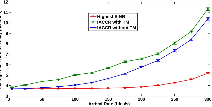
The delay performance shown in Fig. 10 follows a similar trend as the blocking probability. Again, the

highest SINR scheme has the best performance and this is because MSs use the highest SINR possible for transmission and therefore completes transmission faster.

The “IACCR without TM scheme” causes many MSs to

operate at lower SINRs than the highest SINR due to permission of second and third choice connections. Thus, higher average file transfer delay is experienced under the test scheme. The delay is further increased when idle ABSs are allowed to sleep. This is because more distant MS to ABS connections will be experienced and even lower SINRs will be utilized than when idle ABSs are not put into sleep state.

Fig. 9. Blocking probability of baseline scheme and Test scheme without TM and with TM

Fig. 10. Average delay of baseline scheme and test scheme without TM and with TM

0 50 100 150 200 250 300

-0.05 0 0.05 0.1 0.15 0.2 0.25 0.3

Arrival Rate (files/s)

B

lo

c

k

in

g

P

ro

b

a

b

il

it

y

Highest SINR IACCR with TM IACCR without TM

0 50 100 150 200 250 300

3 4 5 6 7 8 9 10 11 12

Arrival Rate (files/s)

A

v

e

ra

g

e

F

il

e

T

ra

n

s

fe

r

D

e

la

y

(

s

e

c

o

n

d

s

)

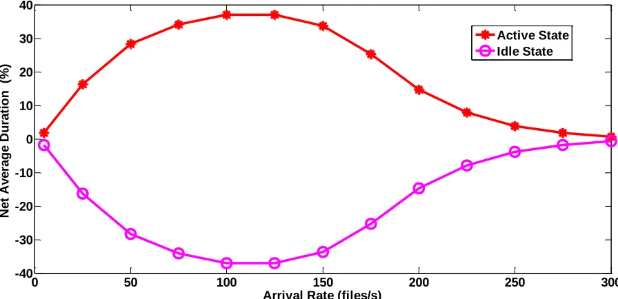
The net average durations of (34), (35), and (36) are normalized by the duration of observation and expressed as percentages. The net average duration of an ABS when sleep state is not permitted (i.e. without TM) is shown in Fig. 11. It is observed at the lowest traffic load (5 files/s) that the net average duration is nearly zero for both active and idle states. This is because a very small number of ABSs is required simultaneously at such a very low traffic load to serve users and there is hardly any room for benefitting from clustering MSs with few ABSs. However, at higher traffic loads (up to 125 files/s) the highest SINR scheme serves MSs with higher number of ABSs (in active state) relative to the test scheme. The test scheme effectively leaves some of the active ABS under the baseline scheme in idle state. Hence, the net average active duration is increasingly positive while the net average idle duration is increasingly negative. Thus, the state difference in this case is only Active to Idle (AI) and it is a power saving LPSS type. As the traffic load increases further the trend is reversed and eventually both net average durations reach zero at 300 files/s. This is as a result of higher interference at higher loads beyond 125 files/s which makes it increasingly difficult for the test scheme to cluster MSs with few ABSs.

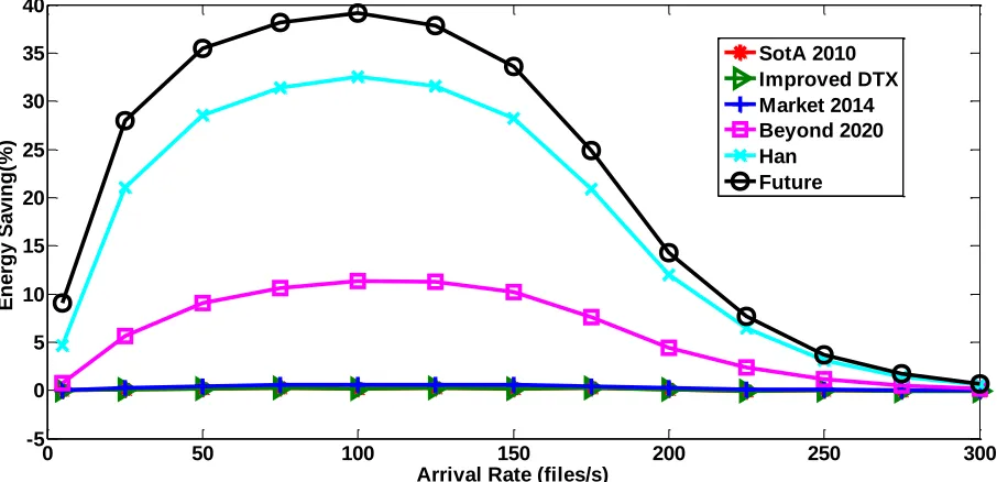
The energy saving for the test scheme without TM is shown in Fig. 12 for the different power models. SotA 2010, Improved DTX and Market 2014 are nearly zero because the LPSS gain for AI is negligible for these power models as explained with the comparative LPSS gain and shown in Fig. 8. However, significant energy saving is achieved with Beyond 2020, Han and Future models, as the LPSS gain for AI is significant for these set of models. The

energy saving trend of these models follows the trend of the net average duration of Fig. 11. It increases as the AI gain increases and decreases when the AI gain decreases. Also, the Future and Han models have higher savings than the Beyond 2020 model. This is because the Future model assumes ABSs have very low idle state consumption like sleep state; while the Han model assumes ABSs have high uplink active consumption. The Beyond 2020 model assumes more moderate idle and active state consumptions, thus the lower saving noticed.

The net average duration of an ABS when sleep state is supported (i.e. with TM) is shown in Fig. 13. It is observed that the net average active duration and the net average idle duration are both positive while the net average sleep duration is negative. Therefore, the state differences in this case are Active to Sleep (AS) and Idle to Sleep (IS) and both state differences are LPSS state differences. The net average active duration (like in the no TM case in Fig. 11) rises from a near zero value at the lowest traffic load to a peak value (at 50 files/s) and then gradually depreciates until it reduces to zero at the highest traffic load. Comparatively, while unused ABSs are left in the idle state in the baseline scheme, in the test scheme these unused ABSs would be put to sleep alongside the active ABSs under the baseline scheme operated in the sleep state under the test scheme for similar time periods. At low loads, the net average idle duration is high but as traffic load increases, the baseline scheme requires more ABSs to be in active state. Thus, the net average idle duration is negligible beyond 100 files/s. As a result below 100 files/s power saving state differences are both AS and IS but mainly AS after 100 files/s.

Fig. 11. Net average duration of ABS for different ABS states when TM is not permitted

0 50 100 150 200 250 300

-40 -30 -20 -10 0 10 20 30 40

Arrival Rate (files/s)

N

e

t

A

v

e

ra

g

e

D

u

ra

ti

o

n

(%

)

Fig. 12. Energy saving of test scheme without TM for different power model assumptions

Fig. 13. Net average duration of ABS for different states when TM is permitted

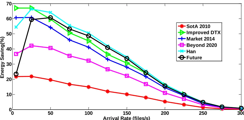
The energy saving for the different power models when TM is applied in the test scheme is shown in Fig. 14. At the lowest load of 5 files/s, as can be observed in Fig. 13, the IS state difference is the predominant power saving state difference because the net average idle duration is significantly higher than the net average active duration. Since the IS state difference gives zero savings for the Future model as shown under the Comparative LPSS of Fig. 8, it has relative low energy saving obtained for the small AS state difference at 5 files/s. However, as the AS state difference duration increases with increasing traffic load, the energy saving increases and reaches its peak when

the AS duration also reaches its peak. Beyond 2020 and Han Models benefit from IS state difference but to lower degree compared to the AS state difference (as observed under Comparative LPSS in Fig. 8). Therefore, both models only reach their peak values after the AS state difference becomes significant. The other models (SotA 2010, Improved DTX and Market 2014) benefit nearly equally from both AS and IS state differences and are therefore at peak values at the lowest traffic load. Energy saving reduces to zero at the highest load when there are no state differences.

0 50 100 150 200 250 300

-5 0 5 10 15 20 25 30 35 40

Arrival Rate (files/s)

E

n

e

rg

y

S

a

v

in

g

(%

)

SotA 2010 Improved DTX Market 2014 Beyond 2020 Han

Future

0 50 100 150 200 250 300

-80 -60 -40 -20 0 20 40 60 80

Arrival Rate (files/s)

N

e

t

A

v

e

ra

g

e

D

u

ra

ti

o

n

(%

)