write-back cache
.
White Rose Research Online URL for this paper:
http://eprints.whiterose.ac.uk/129693/
Version: Published Version
Article:
Davis, Robert Ian orcid.org/0000-0002-5772-0928, Altmeyer, Sebastian and Reineke, Jan
(2018) Response-time analysis for fixed-priority systems with a write-back cache.
Real-Time Systems. ISSN 1573-1383
https://doi.org/10.1007/s11241-018-9305-z
[email protected] https://eprints.whiterose.ac.uk/
Reuse
This article is distributed under the terms of the Creative Commons Attribution (CC BY) licence. This licence allows you to distribute, remix, tweak, and build upon the work, even commercially, as long as you credit the authors for the original work. More information and the full terms of the licence here:
https://creativecommons.org/licenses/
Takedown
If you consider content in White Rose Research Online to be in breach of UK law, please notify us by
https://doi.org/10.1007/s11241-018-9305-z
Response-time analysis for fixed-priority systems with
a write-back cache
Robert I. Davis1,2 · Sebastian Altmeyer3 · Jan Reineke4
© The Author(s) 2018
Abstract This paper introduces analyses of write-back caches integrated into response-time analysis for fixed-priority preemptive and non-preemptive scheduling. For each scheduling paradigm, we derive four different approaches to computing the additional costs incurred due to write backs. We show the dominance relationships between these different approaches and note how they can be combined to form a single state-of-the-art approach in each case. The evaluation explores the relative performance of the different methods using a set of benchmarks, as well as making comparisons with no cache and a write-through cache. We also explore the effect of write buffers used to hide the latency of write-through caches. We show that depending upon the depth of the buffer used and the policies employed, such buffers can result in domino effects. Our evaluation shows that even ignoring domino effects, a substantial write buffer is needed to match the guaranteed performance of write-back caches.
Keywords Write-back cache·Cache-related preemption delays (CRPD)·
Schedulability analysis·Fixed priority scheduling·Real-time
B
Robert I. Davis [email protected]Sebastian Altmeyer [email protected]
Jan Reineke
1 University of York, York, UK 2 INRIA, Paris, France
3 University of Amsterdam, Amsterdam, Netherlands
Extended version
This paper builds upon and extends the RTNS 2016 paperAnalysis of Write-Back Caches under Fixed-Priority Preemptive and Non-preemptive Scheduling(Davis et al. 2016) as follows:
– Worked examples have been added, in Sects.4.3and5.4, illustrating the incom-parability and dominance relationships between the different analysis methods. – A brief discussion of thesustainabilityof the analysis is given in Sect.6. – Additional experiments have been added, in Sect.7.1, exploring how the
perfor-mance of the various analysis methods is impacted by changes in the number of tasks and by the memory delay.
– A discussion and evaluation of the impact of write buffers on the performance of write-through caches has been added in Sect.8. Here we show that depending on the precise policies employed, write buffers may result in domino effects, severely affecting guaranteed performance.
– Finally, while data-cache analysis is not the main focus of the paper, we review related work in this area in the Appendix.
1 Introduction
During the last two decades, applications in aerospace and automotive electronics have progressed from deploying embedded microprocessors clocked in the 10’s of MHz range to higher performance devices operating in the 100’s of MHz to GHz range. The use of high-performance embedded microprocessors has meant that access times to main memory have become a significant bottleneck, necessitating the use of caches to tackle the increasing gap between processor and memory speeds.
Caches may be classified according to the type of information that they store, thus we havedata caches,instruction caches, andunified cacheswhich store both instructions and data. In this paper, we are interested in the behaviour of single-level data and unified caches. The behaviour of these caches is crucially dependent on thewrite policyused. Two policies are commonly employed:write backandwrite through. In caches using a write-through policy, writes immediately go to memory, thus multiple writes to the same location incur an unnecessarily high overhead. In caches using the write-back policy, writes are not immediately written back to memory. Instead, writes are performed in the cache and the affected cache lines are marked asdirty. Only upon eviction of a dirty cache line are its contents written back to main memory. This has the potential to greatly reduce the overall number of writes to main memory compared to a write-through policy, as multiple writes to the same location and multiple writes to different locations in the same cache line can be consolidated.
may occur with non-preemptive as well as with preemptive scheduling, and dirty cache lines left by low priority tasks may impact the response time of higher priority tasks and vice-versa. This is in contrast to the impact of evictions with a write-through cache, which only affect other tasks under preemptive scheduling, and then only tasks of lower priority. In this paper, we discuss different ways of soundly accounting for write backs, and show how to integrate these costs into response-time analysis for both fixed-priority preemptive and non-preemptive scheduling. We also consider the use ofwrite buffersas a way of hiding the write latency inherent in a write-through cache. We show that the use of such buffers can potentially lead todomino effects.
1.1 Related work
1.1.1 Accounting for overheads in schedulability analysis
Early work on accounting for scheduling overheads in fixed-priority preemptive sys-tems by Katcher et al. (1993) and Burns (1994) focused on scheduler overheads and context switch costs. Subsequent work on the analysis of Cache Related Preemption Delays (CRPD) and their integration into schedulability analyses used the concepts of Useful Cache Blocks (UCBs) and Evicting Cache Blocks (ECBs), see Sect. 2.1 of (Altmeyer and Maiza2011) for a detailed description. A number of methods have been developed for computing CRPD under fixed-priority preemptive scheduling. Busquets-Mataix et al. (1996) introduced the ECB-Only approach, which consid-ers just the preempting task; while Lee (1998) developed the UCB-Only approach, which considers just the preempted task (s). Both the UCB-Union approach (Tan and Mooney2007), and the ECB-Union approach (Altmeyer et al.2011) consider both the preempted and preempting tasks. As does an alternative approach developed by Staschulat et al. (2005). These approaches were later superseded by multiset based methods (ECB-Union Multiset and UCB-Union Multiset) which dominate them (Alt-meyer et al.2012). These methods have been adapted by Lunniss et al. (2013,2014a) to EDF scheduling and to hierarchical scheduling with local fixed-priority (Lunniss et al.2014b) and EDF (Lunniss et al.2016) schedulers. They have also been integrated into a response time analysis framework for multicore systems (Altmeyer et al.2015). Cache partitioning is one way of eliminating CRPD; however, this results in inflated worst-case execution times due to the reduced cache partition size available to each task. Altmeyer et al. (2014, 2016) derived an optimal cache partitioning algorithm for the case where each task has its own partition. They compared cache partitioning and cache sharing accounting for CRPD, concluding that the trade off between longer worst-case execution times and CRPD often favours sharing the cache rather than partitioning it.
can share a partition while still avoiding CRPD. This results in a hybrid approach that can outperform the approach of Altmeyer et al. (2014).
As far as we are aware, all of the prior work on integrating CRPD into schedulability analysis assumes write-through caches. In this paper, we explore the impact of using write-back caches instead.
With write-through caches, non-preemptive scheduling provides a simple means of eliminating CRPD without increasing worst-case execution times, since each task can still utilise the entire cache. However, with write-back caches, non-preemptive scheduling is insufficient to eliminate all cache-related interference effects. In this paper, we therefore consider the effects of write-back caches under both fixed-priority preemptive scheduling and fixed-priority non-preemptive scheduling. As this is the
firstsuch study of the impact of write backs, we restrict our attention to direct-mapped caches (examples of microprocessors that implement such caches are given in Sect.2). In future, we aim to extend the techniques to set-associative caches and replacement policies such as LRU using the methodology given by Altmeyer et al. (2011).
1.1.2 Write-back caches in worst-case execution time (WCET) analysis
Ferdinand and Wilhelm (1999) introduced an analysis of write-back caches to deter-mine for each memory access, which cache lines may have to be written back. The basic idea is to track for each potentially dirty memory block whether it must or may be cached; however, this analysis has neither been integrated into a WCET analysis nor has it been experimentally evaluated. Sondag and Rajan (2010) implement a similar idea in the context of multi-level cache analysis, where the write-back behaviour of the first-level cache influences the contents of the second-level cache. While potential write backs from the first- to the second-level cache are correctly accounted for, the
costof write backs to main memory does not seem to be taken into account within their WCET analysis. We note that both approaches (Ferdinand and Wilhelm1999; Sondag and Rajan2010) are not particularly suited to precisely bound thenumberof write backs, as imprecisions in the may- and must-analyses yield many potential write backs for a single write back in a concrete execution. To analyze a program’s WCET, Li et al. (1996) proposed to capture both the software and the microarchitectural behaviour via integer linear programming (ILP). Their analysis is able to cover write-back caches, however, scalability is a major concern. The key distinction between the work pre-sented in this paper and previous research is that our work focuses on the open problem of integrating write-back costs into schedulability analysis. Data cache analysis is not per-se the focus of the work in this paper, nevertheless we provide a discussion of related work in that area in the appendix. For readers interested in cache analysis techniques, a recent survey is given by Lv et al. (2016).
1.2 Organisation
existing response-time analysis techniques. Sections4and5derive analyses bounding the cost of using write-back caches under priority non-preemptive and fixed-priority preemptive scheduling respectively. Section6discusses thesustainabilityof the analysis presented in those sections. Section7provides an evaluation of the per-formance of the different analyses for write-back caches, as compared to no cache and a write-through cache. Section8 discusses the use of write buffers to improve the performance of write-through caches, and evaluates the effectiveness of different sized buffers. Section9discusses how information characterising write-back cache behaviour can be obtained. Finally, Sect.10concludes with a summary and a discus-sion of how the work in this paper may be extended. The appendix provides a brief review of related work on data cache analysis.
2 Caches
Caches are fast but small memories that store a subset of the main memory’s contents to bridge the difference in speed between the processor and main memory. To reduce management overhead and to profit from spatial locality, data is not cached at the granularity of words, but at the granularity of so-calledmemory blocks. To this end, main memory is logically partitioned into equally-sized memory blocks. Blocks are cached incache linesof the same size. The size of a memory block varies from one processor to another, but is usually between 32 and 128 bytes.
When accessing a memory block, the cache logic has to determine whether the block is stored in the cache, acache hit, or not, acache miss. To enable an efficient look-up, each memory block can only be stored in a small number of cache lines referred to as acache set. Thus caches are partitioned into a number of equally-sized cache sets. The size of a cache set is called theassociativityof the cache.
Theplacement policydetermines the cache set a memory block maps to. Typically, the number of cache sets is a power of two, andmodulo placement is employed, where the least significant bits of the block number determine the cache set that a memory block maps to. Since caches are usually much smaller than main memory, a
replacement policyis used to decide which memory block to replace on a cache miss. As stated earlier, we limit our attention todirect-mappedcaches, where each cache set consists of exactly one cache line. In this case, the only possible action on a cache miss is to replace the memory block currently stored in the cache line that the accessed memory block maps to.
In this paper, we assume a timing-compositional architecture (Hahn et al.2013), i.e. the timing contribution of cache misses and write backs can be analyzed separately from other architectural features such as the pipeline behaviour.
2.1 Write policies
to main memory is postponed until the memory block containing the data is evicted from the cache, it is then written back to main memory in its entirety.
Write through is simpler to implement than write back, but may result in a signifi-cantly larger number of accesses to main memory. If a cached memory block is written to multiple times before being evicted, under write back only the final write needs to be performed to main memory. The drawback of write-back caches is that additional
dirtybits are required to keep track of which cache lines have been modified since they were fetched from main memory, the writes are delayed, and the logic required to implement the cache is more complex.
Due to the potential performance advantages of write-back caches they are often preferred in embedded microprocessor designs. Alternatively, caches may be con-figurable as write back or write through. Examples include: Infineon Tricore TC1M (separate data and instruction caches, LRU replacement policy, write back); Freescale MPC740 (separate data and instruction caches, PLRU replacement policy, config-urable for write back or write through); Renesas SH7705 (unified data and instruction cache, LRU replacement policy, configurable for write back or write through); Rene-sas SH7750 (separate instruction and data caches, direct mapped, configurable for write back or write through); NEC VR4181 and VR4121 (separate instruction and data caches, direct mapped, write back).
A second question to answer when designing a cache is what happens on a write to a memory block that is not cached. There are twowrite-miss policies: Withwrite allocate a cache line is allocated to the memory block containing the word that is being written, which is fetched from main memory, then the write is performed in the cache. Withno-write allocatethe write is performed only in main memory, and no cache line is allocated. In principle, each write policy can be used in conjunction with each write-miss policy; however, usually, write through is combined with no-write allocate, and write back is combined with write allocate. In this paper we assume a cache employingwrite backandwrite allocate, which minimizes the total number of accesses to main memory.
2.2 Classification of write backs
For analysis purposes, it is useful to classify write backs into three categories:
Job-internal write backs. These are write backs of dirty cache lines previously written to by the same job. We assume that the cost of job-internal write backs is included in the WCET of a task, since it does not depend on the scheduling policy used.
a
Write backs:
c∗
b∗
d d∗
a b
a d f b f d
carry-in
job-internal
preemption-induced
f∗
d d∗ c∗
f∗
a∗
c Taskτ1
Taskτ2
Taskτ3
c
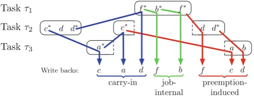
Fig. 1 Example illustrating different kinds of write backs
from finished jobs can emanate from both lower and higher priority tasks. We refer to these as “finished-carry-in” write backs.
Preemption-induced write backs. These are write backs of dirty cache lines that were not written to by the task itself and that were introduced by a preempting task. Preemption-induced write backs can only come from higher priority jobs that are finished.
Consider Fig.1for an example schedule of three tasks containing the three types of write backs described above. In the example,x∗denotes a write to memory blockx, whereas justxdenotes a read from memory blockx. Memory blocksa,candb,d, f
map to the same cache sets, and hence cache lines, respectively.
The first write to memory blocka of taskτ3, causes the eviction ofc, which was
written to by a finished job of taskτ2, thus it causes afinished-carry-inwrite-back. On
the other hand, the access tocin the second job ofτ2, causes anlp-carry-inwrite back
ofa. The first access tobwithin taskτ1evicts f, which was previously modified in the
same job, thus causing ajob-internalwrite back. Finally, the read ofdin the second job of taskτ2causes apreemption-inducedwrite back of f which was previously written
to by taskτ1. Similarly, the reads ofa andbin taskτ3result in preemption-induced
write backs ofcandd, previously written to by taskτ2.
2.3 Characterizing a task’s write backs
We assume that job-internal write backs are accounted for within WCET analysis. To bound carry-in write backs, and in the case of preemptive scheduling, preemption-induced write backs, we need to characterize the memory-access behaviour of each task. To do so, we introduce the following concepts:
AnEvicting Cache Block(ECB) of taskτiis a memory block that may be accessed
by taskτi. We denote the set of cache lines that evicting cache blocks of taskτimap to
byEC Bi. Note ECBs have previously been considered in the analysis of cache-related
preemption delays (Altmeyer et al.2012).
ADirty Cache Block(DCB) of taskτi is a memory block that may be written to
by taskτi. We denote the set of cache lines that dirty cache blocks of taskτi map to
[image:8.439.91.349.56.157.2]AFinal Dirty Cache Block(FDCB) of taskτi is a DCB that may still be cached at
completion of the task. We denote the set of cache lines that final dirty cache blocks of taskτi map to byF DC Bi. (By definition,F DC Bi ⊆DC Bi ⊆EC Bi).
By evicting dirty cache lines, ECBs may cause both carry-in and preemption-induced write backs. In preemptive scheduling, lp-carry-in write backs may occur due to DCBs, while preemption-induced and finished-carry-in write backs can only be due to FDCBs. In non-preemptive scheduling, preemption-induced write backs do not occur, and carry-in write backs are necessarily finished-carry-in write backs, and can thus only be due to FDCBs. With both scheduling paradigms, job-internal write backs can occur and carry-in write backs can occur due to jobs of all tasks, including the previous job of the same task.
3 Task model and basic analysis
In this section, we set out the basic task model used in the rest of the paper, and recapitulate existing response-time analyses for fixed-priority preemptive scheduling (FPPS) and fixed-priority non-preemptive scheduling (FPNS).
3.1 Task model
We consider a set of sporadic tasks scheduled on a uniprocessor under either FPPS or FPNS. A task setŴcomprises a static set ofn tasks{τ1, τ2, . . . , τn}. Each task has
a unique priority, which without loss of generality is given by its index. Thus taskτ1
has the highest priority and taskτnthe lowest. Each taskτigives rise to a potentially
unbounded sequence of jobs separated by a minimum inter-arrival time or periodTi.
Each job of taskτihas a bounded worst-case execution timeCi, and relative deadline Di. Deadlines are assumed to beconstrained, i.e.Di ≤Ti. NoteCi is the worst-case
execution time in the non-preemptive case, starting from an arbitrary clean cache. ThusCidoes not include the cost of reloading cache lines evicted due to preemption,
or additional write backs that may be required when loading memory blocks into dirty cache lines. On the other hand, it does include the cost of job-internal write backs.
The worst-case response time Ri of taskτi is given by the longest time from the
release of a job of the task until it completes execution. If the worst-case response time is not greater than the deadline (Ri ≤Di), then the task is said to be schedulable. The utilizationUi of a taskτi is given byUi = CTi
i and the utilization of the task set is the
sum of the utilizations of the individual tasksU=ni=1Ui.
We usehp(i)andhep(i)to denote respectively the set of indices of tasks with priorities higher than, and higher than or equal to that of taskτi (includingτi itself).
3.2 Schedulability analysis for FPPS
For task sets with constrained deadlines scheduled using FPPS, the exact response time of taskτi may be computed according to the following recurrence relation (Audsley
et al.1993; Joseph and Pandya1986):
RiP =Ci + j∈hp(i)
RiP
Tj
Cj (1)
Iteration starts with RiP =Ci and ends either on convergence or whenRiP >Di in
which case the task is unschedulable.
3.3 Schedulability analysis for FPNS
Determining exact schedulability of a taskτi under FPNS requires checking all of the
jobs of taskτi within the worst-case priority level-i busy period (Bril et al.2009).
(This is the case even when all tasks have constrained deadlines).
The worst-case priority level-i busy period starts with an interval of blocking due to a job of the longest task of lower priority thanτi. Just after that job starts to execute,
jobs of taskτi and all higher priority tasks are released simultaneously, and then
re-released as soon as possible. Finally, the busy period ends at some timetwhen there are no ready jobs of priorityior higher that were not released strictly before timet.
In this paper, we make use of the followingsufficientschedulability test for FPNS, applicable only to constrained-deadline task sets. It is based on a test originally given for non-preemptive scheduling on Controller Area Network (CAN) (Davis et al.2007). This schedulability test considers two scenarios. Either the worst-case response time for taskτioccurs for the first job in the priority level-ibusy period, or for a subsequent
job. The start timeWiN P,0 of the first jobq =0 of taskτi in the worst-case priority
level-i busy period can be computed using the following recurrence relation:
WiN P,0 = max
k∈l p(i)Ck+
j∈hp(i)
WiN P,0
Tj
+1 Cj (2)
and hence its worst-case response time is given by:
RiN P,0 =WiN P,0 +Ci (3)
Subsequent jobs of task τi may be subject topush-through blocking due to
non-preemptive execution of the previous job of the same task. Let the jobs of taskτi be
indexed by values ofq =0,1, . . ., whereq =0 is the first job in the busy period. We consider jobq+1, assuming that jobqis schedulable (we return to this point later). Since jobqis schedulable it completes by its deadline at the latest and therefore also by the release of jobq+1. Consider the length of the time interval from when jobq
there can be no jobs of higher priority tasks that are ready to execute. In the worst-case, jobs of all higher priority tasks may be released immediately after jobqstarts to execute. Thus an upper bound on the lengthWiN P,q+1of this interval can be computed using the following recurrence relation:
WiN P,q+1=Ci+ j∈hp(i)
WiN P,q+1
Tj
+1 Cj (4)
Since we assume that jobq completes by its deadline and deadlines are constrained (Di ≤Ti), then the intervalWiN P,q+1must also upper bound the time from the release of jobq+1 until it starts to execute. As jobq+1 takes timeCito execute, an upper
bound on its worst-case response time is given by:
RiN P,q+1=WiN P,q+1+Ci (5)
Assuming that jobq = 0 is schedulable according to (2) then schedulability of the second and subsequent jobs in the busy period can be determined by induction using (5).
We note the similarity between (2) and (4), and also between (3) and (5). Thus we may combine them obtaining an upper bound for the response time of taskτi, under
FPNS. This upper bound may be compared with the task’s deadline to determine schedulability.
WiN P = max
k∈lep(i)Ck+
j∈hp(i)
WiN P
Tj
+1 Cj (6)
RiN P =WiN P+Ci (7)
The analysis expressed in (5) can be improved by noting that the start time of jobq
must be at leastCi before the release of job q+1, hence the response time upper
bound given in (5) may be reduced byCi. In this paper, for ease of presentation, we
make use of the simpler test embodied in (6) and (7).
4 Write backs under FPNS
In this section, we extend the sufficient schedulability test for FPNS for constrained-deadline task sets given in (6) and (7) to account for carry-in write backs. In non-preemptive scheduling only job-internal and finished-carry-in write backs may occur. As discussed earlier, we assume that job-internal write backs are accounted for within WCET analysis.
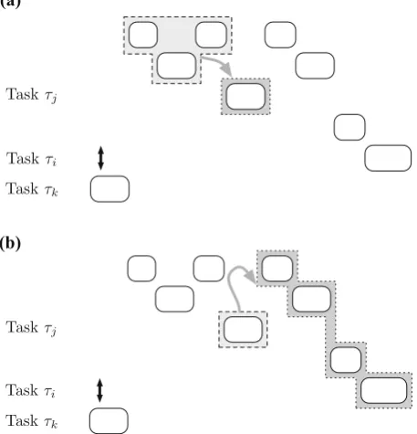
We identify two methods of accounting for finished-carry-in write backs, which are illustrated in Fig.2. In the first method, we associate with each job of a task, the carry-in write backs that occurwithin the job. This method is used in theECB-Onlyand
Taskτj
Taskτi
Taskτk
(a)
Taskτj
Taskτk
Taskτi
(b)
Fig. 2 Carry-in write backs may be accounted for either,awithin the job of the taskτiunder analysis, or
bin subsequent jobs of both higher (e.g.τj) and lower (e.g.τk) priority tasks
associate with each job of a task the carry-in write backs that occur insubsequent jobs
due to dirty cache lines left by the job itself. This method is used in theFDCB-Only
andECB-Unionapproaches described in Sect.4.2.
4.1 Carry-in write backs within the job
4.1.1 ECB-Only approach
The number of ECBs provides an upper bound on the number of carry-in write backs a task suffers.1Thus, assuming timing compositionality (Hahn et al.2013), the WCET of taskτi, including the cost of write backs, is bounded by
Ci′=Ci+W BT · |EC Bi| (8)
whereW BT is an upper bound on the time to perform one write back. ReplacingCi
byCi′as defined above (and similarlyCk andCj), (6) and (7) can be used to derive
worst-case response times accounting for write backs.
1 Note that this holds for direct-mapped caches as well as for set-associative caches with LRU replacement.
[image:12.439.106.335.62.300.2]4.1.2 FDCB-Union approach
The ECB-Only approach can be improved upon by taking into account which cache lines may be dirty when a job is started. In non-preemptive execution, dirty cache lines at a job’s start are the final dirty cache lines left by other jobs.
When analyzingτi’s response time, we distinguish two types of finished-carry-in
write backs: Those that are due to dirty cache lines introduced beforeτi’s release by
tasks with lower or equal priority toτi, represented byδi, and those that are due to
dirty cache lines introduced before and afterτi’s release by tasks of higher priority
thanτi, represented byγiwb,j.
Each final dirty cache line of a task with priority lower than or equal to that of task τi may result in at most one write back duringτi’s response time, excluding write
backs that occur during the blocking time. Write backs of these dirty cache lines can only occur within the response time of taskτi if the cache lines are accessed by (i.e.
in theEC Bk) some taskτkof priorityior higher. The termδiaccounts for these write
backs. Note that we exclude fromδicache lines that may be dirty due to higher priority
tasks as such cache lines are accounted for by theγiwb,j term introduced next, thus:
δi =W BT · ⎛ ⎝
k∈lep(i)
F DC Bk\
k∈hp(i)
F DC Bk ⎞
⎠∩ ⎛
⎝
k∈hep(i)
EC Bk ⎞ ⎠ (9)
The number of finished-carry-in write backs that can be made during the execution of one job of taskτj due to dirty cache lines introduced by tasks of higher priority
thanτi is upper bounded byγiwb,j. Note that only cache lines accessed by taskτj (i.e.
inEC Bj) can be written back during the execution of a job ofτj.
γiwb,j =W BT · ⎛ ⎝
k∈hp(i)
F DC Bk ⎞
⎠∩EC Bj (10)
We now adapt (6) and (7) to include the write backs (γn+wb1,b) that can occur within one job of a blocking taskτb; the write backs (δi) that can occur during jobs other than
that of a blocking task, due to dirty cache lines left by tasks of lower priority thanτi
before the start of the busy period; and finally, the write backs (γiwb,j andγiwb,i ) that can occur within each of the other jobs that contribute to the response time of taskτi, due
to dirty cache lines introduced by tasks of higher priority thanτi.
WiN P,W B= max
b∈lep(i)
Cb+γn+wb1,b+ δi
+
j∈hp(i)
WiN P,W B
Tj
+1 Cj+γiwb,j
(11)
RiN P,W B=WiN P,W B+Ci +γiwb,i
In theγn+wb1,bterm,n+1 denotes a priority that is lower than that of any task, thus γn+wb1,baccounts for all carry-in write backs that may occur during the execution of a blocking taskτbdue to cache lines left dirty by previous jobs of any task. In contrast,
γiwb,j andγiwb,i need only cover write backs due to dirty cache lines from tasks of higher priority thanτi, since all other write backs are accounted for inδi.
The ECB-Only approach pessimistically assumes that each time a task is executed the cache is full of dirty cache lines. The FDCB-Union approach improves upon this by more precisely modeling which cache lines could actually be dirty. FDCB-Union strictly dominates ECB-Only, meaning that any task set that is deemed schedulable according to the ECB-Only approach is guaranteed to be deemed schedulable using the FDCB-Union approach. This can be seen by first considering theCj+γiwb,j terms
in (11) and (12). From (10), it follows that Cj +γxwb,j cannot be greater than the
value ofC′j used in (8) for any taskτj and indexx, and hence cannot exceed the
inflated WCET values used in the ECB-Only approach. Second, we must consider the additional contributions in theδi term. For an FDCB to contribute toδi, then from
(9), that FDCB cannot be inF DC Bkof any taskτkwith a priority higher than that of
taskτi. Also, it must be in theEC Bi of taskτior theEC Bkof some higher priority
taskτk. If it is in EC Bi and contributes toδi then from (10) it is not included in the
γiwb,i term in (12), thus the inflated WCETCi′in the ECB-Only approach covers both this contribution toδi and theγiwb,i term in (12). Similarly, if the FDCB is inEC Bj
and contributes toδi then it is not included in theγiwb,j term in (11), thus the inflated
WCETC′jin the ECB-Only approach again covers both this contribution toδandγiwb,j. Finally, it serves only to consider a system with no FDCBs to see that FDCB-Union strictly dominates ECB-Only. At the other extreme, if all ECBs are also FDCBs, then FDCB-Union reduces to ECB-Only (withδi =0).
4.2 Carry-in write backs in subsequent jobs
4.2.1 FDCB-Only approach
Instead of usingγiwb,j to mean the cost of carry-in write backs that occurwithinthe execution of a job of taskτj, we can re-defineγiwb,j to cover the write backs that occur
insubsequent jobsdue to dirty cache lines left by a job of taskτj. This is achieved by
assuming that all of these cache lines may be evicted by the subsequent jobs:
γiwb,j =W BT ·F DC Bj
(13)
With this approach,δneeds to account forallcarry-in write backs due to cache lines that were dirty prior toτi’s release:
δ=W BT ·
k
F DC Bk
Finally, the final dirty cache lines thatτi leaves do not affect its own response time.
As a consequence (12) can be simplified as follows (with (11) unchanged):
RiN P,W B=WiN P,W B+Ci (15)
4.2.2 ECB-Union approach
The above approach can be improved by taking into account which of the dirty cache lines may actually be evicted by subsequent jobs of tasks which may execute within τi’s response time (i.e. by also considering the cache lines (EC Bk) accessed by each
taskτk of priorityi or higher).
γiwb,j =W BT ·
F DC Bj ∩ ⎛
⎝
k∈hep(i)
EC Bk ⎞ ⎠ (16)
Similarly, in theδb,i term, we need only account for those dirty cache lines that may
be evicted duringτi’s response time. This depends on the blocking taskτb:
δb,i =W BT · k
F DC Bk ∩ ⎛
⎝
j∈hep(i)∪{b} EC Bj
⎞ ⎠ (17)
Hence we includeδb,i in the blocking term resulting in the following adaptation of
(11):
WiN P,W B= max
b∈lep(i)(Cb+γ
wb i,b +δb,i
+
j∈hp(i)
WiN P,W B
Tj
+1 (Cj+γiwb,j)
(18)
The ECB-Union approach strictly dominates the FDCB-Only approach. This can be seen by comparing theγiwb,j terms and theδb,i terms. Comparing theγiwb,j terms in
(13) and (16) we note that surprisingly there is no advantage gained by ECB-Union, sinceF DC Bj ⊆EC Bjandi ∈lep(j)in all uses of this term, hence (16) effectively
reduces to (13). Considering theδb,i terms, if there are a number of lower priority
tasks with FDCBs that are not present in the ECBs of tasks with priorities higher than or equal toτi then (17) can improve upon (14), with dominance apparent from the set
intersection.
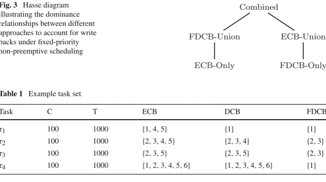
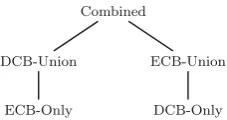
Fig. 3 Hasse diagram illustrating the dominance relationships between different approaches to account for write backs under fixed-priority non-preemptive scheduling
Combined
FDCB-Union
ECB-Only
ECB-Union
[image:16.439.52.387.57.244.2]FDCB-Only
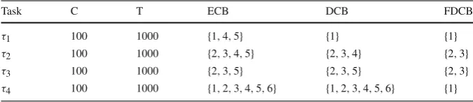
Table 1 Example task set
Task C T ECB DCB FDCB
τ1 100 1000 {1,4,5} {1} {1}
τ2 100 1000 {2,3,4,5} {2,3,4} {2,3}
τ3 100 1000 {2,3,5} {2,3,5} {2,3}
τ4 100 1000 {1,2,3,4,5,6} {1,2,3,4,5,6} {1}
4.3 Worked example
Below, we present a worked example illustrating the various approaches to analysing write backs under fixed-priority non-preemptive scheduling and their differences in performance. Table1gives the task set parameters.
For ease of presentation, we assume a write-back delay of 1 and choose task param-eters so that only one job of each task may be released during another task’s response time. The sets of UCBs are assumed to be empty (i.e. we focus on write backs and do not consider CRPD due to cache misses).
4.3.1 ECB-Only
The ECB-Only approach (8) effectively increases the tasks’ execution times byW BT· |EC B|:C1′ = 103,C′2 = 104,C′3 = 103,C4′ = 106. The response time is then computed using (6) and (7) givingR1=209,R2=313,R3=416, andR4=522.
4.3.2 FDCB-Union
The FDCB-Union approach extends the ECB-Only approach by taking into account which cache lines may be dirty when a job is started. The termδi accounts for dirty
cache lines of lower or equal priority tasks and is computed using (9):δ1=1, δ2=
2, δ3=0, δ4=0. The termγiwb,j accounts for write backs due to higher priority tasks
and is computed using (10):
γiwb,j 1 2 3
2 1− −
3 1 2 −
[image:16.439.50.390.165.237.2]Further, we have:γ5wb,1 =1,γ5wb,2 =2,γ5wb,3 =2,γ5wb,4 =3 andγ1wb,1 =0,γ2wb,2 =0, γ3wb,3 =2,γ4wb,4 =3. The response time is then computed using (11) and (12) giving
R1=204,R2=306,R3=408, andR4=511.
Note that the FDCB-Union approach dominates ECB-Only and results in shorter response times in this example.
4.3.3 FDCB-Only
The FDCB-Only approach accounts for write backs in subsequent jobs, instead of write backs in the execution of the job itself. Hence, the term δ accounts for dirty cache lines prior to the release of the task under analysis and is given by (14) thus δi =3. Theγiwb,j term is given by (13):
γiwb,j 1 2 3
2 1− −
3 1 2 −
4 1 2 2
Further,γ5wb,1 =1,γ5wb,2 =2,γ5wb,3=2,γ5wb,4 =1. The response time is then computed using (11) and (15) givingR1=205,R2=306,R3=408, andR4=509.
4.3.4 ECB-Union
The ECB-Union approach only differs from FDCB-Only in theδ terms. This dif-ference, although technically possible, is neither visible in this example, nor in the evaluation. Instead, the ECB-Union approach results in the same response times as the FDCB-Only approach.
We observe that this example suffices to highlight the incomparability between ECB-Union and FDCB-Union. The response time for taskτ1is smaller with
FDCB-Union (204 vs. 205), while the response time for taskτ4is smaller with ECB-Union
(509 vs. 511). The combined approach, taking the minimum response times (204, 306, 408, 509) thus dominates all others.
5 Write backs under FPPS
Response-time analysis for FPPS has previously been extended to account for preemption-related cache misses (Altmeyer et al.2011, 2012) by introducing a term γi,j into the response-time equation for taskτias follows:
RiP =Ci+ j∈hp(i)
RiP
Tj
To also account for additional write backs in preemptive scheduling, we extend the recurrence relation as follows:
RiP =δi +Ci+
j∈hp(i)
R i Tj
Cj+γimiss,j +γ wb i,j
(20)
Here,δi is used to account for write backs due to cache lines that were already dirty
on release ofτiand are written back within its response time. Additional cache misses
due to preemptions are captured byγimiss,j . Any of the existing techniques, for example those introduced by Altmeyer et al. (2012), can be used to account for such misses. Finally,γiwb,j is used to account for carry-in and preemption-induced write backs of cache lines that were written to afterτi’s release.
We further sub-divideγiwb,j intoγiwb-lp,j andγiwb-fin,j , such thatγiwb,j =γiwb-lp,j +γiwb-fin,j ,
whereγiwb-lp,j accounts for lp-carry-in write backs andγiwb-fin,j accounts for finished-carry-in and preemption-induced write backs (see Sect.2.2for their definitions). In the following we introduce four different ways of computingγiwb-lp,j . These combine with the analysis derived forδiandγiwb-fin,j to give theDCB-Only,ECB-Union,ECB-Only
andDCB-Unionapproaches for analysing write backs under FPPS.
5.1 Initially dirty cache line write backs
We first consider which cache lines may be dirty when the priority level-ibusy period starts that leads to the worst-case response time of a job of taskτi. Only tasks of lower
priority thanτimay be active immediately before the start of this busy period, so the
cache lines in
j∈l p(i)DC Bj may all be in the cache and dirty. Further, the cache
lines in
k∈hep(i)F DC Bkmay have been left dirty by finished jobs of higher priority
tasks. Among all the dirty cache lines, we need only account for those that may be evicted withinτi’s response time. As onlyτi and higher priority tasks can run during
this interval, these are
k∈hep(i)EC Bk, hence we obtain the following formula forδi:
δi =W BT· ⎛ ⎝
j∈lp(i)
DC Bj∪
k∈hep(i)
F DC Bk ⎞
⎠∩ ⎛
⎝
k∈hep(i)
EC Bk ⎞ ⎠ (21)
5.2 Lower priority carry-in write backs
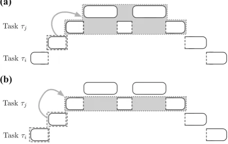
To bound lp-carry-in write backs (γiwb-lp,j ) due to preempted tasks, we identify two methods, both illustrated in Fig.4.
(a) the lp-carry-in write backs of dirty cache lines introduced by the job immediately-preempted by a job of τj that occur within the response time ofτj, i.e. either
Taskτj
Taskτi
Taskτj
Taskτi (a)
(b)
Fig. 4 Methods of accounting for lp-carry-in write backs.aEffect of immediately-preempted task (light grey) on all preempting tasks (dark grey).bEffect of preempted tasks (light grey) on immediately preempting task (dark grey)
(b) the lp-carry-in write backs of dirty cache lines introduced byany preempted lower priority tasksthat occur within the execution of a job ofτj.
Using method (a), we define the DCB-Only and ECB-Union approaches, and with method (b), the ECB-Only and DCB-Union approaches.
5.2.1 DCB-Only approach
Using method (a), any task that could be active during the response time of taskτi and
has a lower priority than taskτj(i.e. a task in the setaff(i,j)=hep(i)∩l p(j)) could
be immediately preempted by taskτj, thus we obtain the following upper bound on
the cost of write backsγiwb-lp,j associated with jobs of taskτj:
γiwb-lp,j =W BT· max
h∈aff(i,j)|DC Bh| (22)
Note, when using this DCB-Only approach we assume that (21) is simplified ignoring the ECBs.
δi =W BT ·
j∈lp(i)
DC Bj ∪
k∈hep(i)
F DC Bk
(23)
5.2.2 ECB-Union approach
[image:19.439.106.334.60.204.2]active, i.e. due to execution ofτj or a higher priority task (see Fig.4) thus:
γiwb-lp,j =W BT · max
h∈aff(i,j)
DC Bh∩ l∈hep(j)
EC Bl (24)
5.2.3 ECB-Only approach
Using method (b), the lp-carry-in write backs of dirty cache lines introduced byany preempted lower priority tasksthat occur within the execution ofτjare upper bounded
by the ECBs ofτj:
γiwb-lp,j =W BT ·EC Bj
(25)
Note, when using this ECB-Only approach we assume that (21) is simplified ignoring the DCBs.
δi =W BT·
k∈hep(i)
EC Bk (26)
5.2.4 DCB-Union approach
The ECB-Only approach can be refined by noting that we are only interested in write backs of dirty cache lines introduced bypreempted lower priority tasks(see Fig.4). Note, that we do not need to account for lp-carry-in write backs due to dirty cache lines of tasks of lower priority thanτi as these are already accounted for inδi.
γiwb-lp,j =W BT · ⎛ ⎝
h∈aff(i,j)
DC Bh ⎞
⎠∩EC Bj (27)
5.3 Finished-carry-in write backs
A job of taskτj can leave|F DC Bj|dirty cache lines, which may have to be written
back withinτi’s response time. This yields the following simple bound on the cost of
finished-carry-in and preemption-induced write backs:
γiwb-fin,j =W BT · |F DC Bj|. (28)
One might assume that this bound can be improved by taking into account the evicting cache blocks of other tasks; however, as F DC Bj ⊆ EC Bj, then without
further information, we must assume that the next job of taskτj will have to clean up
Fig. 5 Hasse diagram illustrating the dominance relationships between approaches to account for write backs under fixed-priority preemptive scheduling
Combined
DCB-Union
ECB-Only
ECB-Union
DCB-Only
By construction, the ECB-Union approach dominates Only, and the DCB-Union approach dominates ECB-Only. Further, since ECB-DCB-Union and DCB-DCB-Union are incomparable we may form a combined approach that takes the smallest response time computed by either approach, and hence dominates both. Figure 5 illustrates these relationships via a Hasse diagram.
In some cases there could be pessimism in the analysis for FPPS as a result of write backs that are counted as both job-internal write backs in the WCET of a task, and also as carry-in write backs that occur when a task is preempted and a cache line is written back by the preempting task. As an example consider the sequence of accessesc∗,c∗,
c∗,dwhere memory blockscanddare mapped to the same cache line, and∗indicates a write. Here the read ofdcauses a job-internal write back ofc. Preemption between the final write tocand the read ofdcould result in the preempting task writing backc
(a carry-in write back), but no job-internal write back. In this case the analysis would over-approximate the total number of write backs. However, preemptions between the writes toccould induce a further carry-in write back in addition to the job-internal one. While there is some over-approximation in the analysis, our evaluations, in the next section, show that this over-approximation is small, with the combined approach close to the upper bound computed without write-back costs.
5.4 Worked example
Below, we present a worked example illustrating the various approaches to analysing write backs under fixed-priority preemptive scheduling and their differences in per-formance. Table2gives the task set parameters. (Note the example task set is the same as that used in Sect.4.3. It is repeated here for ease of reference).
For ease of presentation, we again assume a write-back delay of 1 and choose task parameters so that only one job of each task may be released during another task’s response time. The sets of UCBs are assumed to be empty.
In the case of fixed-priority preemptive scheduling, all four approaches use the same response time equation (20), and the sameγiwb-fin,j terms to account for the finished carry-in write backs (28):γ_wb-fin,1 = 1,γ_wb-fin,2 = 2,γ_wb-fin,3 = 2,γ_wb-fin,4 = 1. The approaches only differ in theδi terms to account for initially dirty cache lines and the
[image:21.439.274.388.58.118.2]Table 2 Example task set
Task C T ECB DCB FDCB
τ1 100 1000 {1,4,5} {1} {1}
τ2 100 1000 {2,3,4,5} {2,3,4} {2,3}
τ3 100 1000 {2,3,5} {2,3,5} {2,3}
τ4 100 1000 {1,2,3,4,5,6} {1,2,3,4,5,6} {1}
5.4.1 DCB-Only
Uses (23) to compute:δ1=6,δ2=6,δ3=6,δ4=3.
γiwb-lp,j 1 2 3
2 3− −
3 3 3 −
4 6 6 6
R1=106,R2=210,R3=315,R4=426.
5.4.2 ECB-Union
Uses (21) to compute:δ1=3,δ2=5,δ3=5,δ4=3.
γiwb-lp,j 1 2 3
2 1− −
3 1 3 −
4 3 5 5
R1=103,R2=207,R3=312,R4=421.
5.4.3 ECB-Only
Uses (26) to compute:δ1=3,δ2=5,δ3=5,δ4=6.
γiwb-lp,j 1 2 3
2 3− −
3 3 4 −
4 3 4 3
5.4.4 DCB-Union
Uses (21) to compute:δ1=3,δ2=5,δ3=5,δ4=3.
γiwb-lp,j 1 2 3
2 1− −
3 2 3 −
4 3 4 3
R1=103,R2=207,R3=313,R4=418.
The example shows the dominance relationships of ECB-Union over DCB-Only and DCB-Union over ECB-Only, as well as the incomparability between ECB-Union and DCB-Union. The response time for taskτ3is smaller with ECB-Union than with
DCB-Union (312 vs. 313). Vice versa, the response time for taskτ4is smaller with
DCB-Union than with ECB-Union (418 vs. 421). The combined approach, taking the minimum response times (103, 207, 312, 418) thus dominates all others.
6 Sustainability of the analysis
The analysis given in this paper builds upon response-time analyses for FPPS and FPNS (see Sects.3.2and3.3respectively), integrating the effects of write-back costs. The response-time analyses used for FPPS and FPNS are bothsustainable(Baruah and Burns2006), meaning that a system that is deemed schedulable by the schedu-lability test used will not become unschedulable or be deemed unschedulable by the test if the task parameters areimproved. These improvements include (i) reduced exe-cution times, (ii) increased periods or minimum inter-arrival times, and (iii) increased deadlines.
We note that with the integration of write-back costs and CRPD given in Sects.4and 5, sustainability still holds with respect to the above parameters. Further, the analysis is sustainable with respect to improvements in the sets of cache lines considered, i.e. ECBs, DCBs, and FDCBs. (Here, by improvement we mean removal of one or more elements from a set, such that the new set is a subset of the old). This can be seen from the formulaes involved, since the response times computed are monotonically non-decreasing with respect to increases (addition of elements) to any of these sets. In all of the equations given in Sects.4and5, for the overheads of write backs, the ECBs, DCBs, and FDCBs are combined using union, intersection, and cardinality operators. Thus the overheads are monotonically non-decreasing with respect to the content of those sets, and so any response timeR′i computed usingEC B′j,DC B′j,F DC B′j is no smaller thanRicomputed usingEC Bj,DC Bj,F DC Bj whereEC B′j ⊇EC Bj, DC B′j ⊇ DC Bj, andF DC B′j ⊇F DC Bj. The only exception that requires further
consideration occurs in the FDCB-Union approach (Sect.4.1) where (9) makes use of the set subtraction operator. Here, any reduction in the value ofδidue to an additional
element inF DC Bkwherek∈hp(i)is matched by an increase inγiwb,j given by (10)
priority task is included in the response time equation (11) at least once, the computed response time cannot decrease with the addition of any element toF DC Bj.
7 Experimental evaluation
In this section, we evaluate the performance of the different analyses introduced in Sects. 4 and5 for write-back caches under fixed-priority preemptive and non-preemptive scheduling, as compared to no cache and a write-through cache. For both write-back and write-through caches, we assumed a write-allocate policy. Preliminary experiments showed that the difference between write allocate and no-write allocate for a write-through cache were minimal, with the former giving slightly better perfor-mance on the benchmarks studied.
We assume a timing-compositional processor with separate instruction and data caches. Each cache is direct-mapped and has 512 cache lines of size 32 bytes. Thus both caches have a capacity of 16 KB. Further, we assume a write-back latencyW BT
of 10 cycles. Cache misses also take 10 cycles, while non-memory instructions and cache hits take 1 cycle.
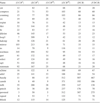
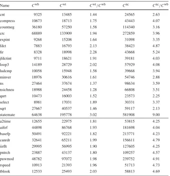
As aproof-of-conceptfor the analysis techniques, we obtained realistic estimates for WCETs and the sets of DCBs and ECBs, from the Mälardalen benchmark suite (Gustafsson et al.2010) and the EEMBC Benchmark suite (EEMBC2016) (Sect.9 explains how this was done). Table3shows the WCETs (without inter-task interfer-ence) assuming a write-back cache (Cwb), a write-through cache (Cwt), and no data cache (Cnc) for the selected benchmarks. Table4shows the number of UCBs, ECBs, DCBs, and FDCBs. We note that these stand-alone WCETs are a substantial factor of 1.4 to 3.0 times lower with a write-back cache than with write through, and 2 to 9 times lower than with no data cache. Since we assume a separate instruction and data cache, the UCB and ECB values are shown separately for each cache.
We note that fixed-priority non-preemptive scheduling suffers from the long task problem, whereby task sets that contain some tasks with short deadlines and others with long WCETs are trivially unschedulable due to blocking. To ameliorate this problem, we only selected benchmarks for Table4where the stand-alone WCETs were in the range[7000:70,000]cycles. This interval corresponds to the most populated range where the smallest and largest WCETs differ by a factor of 10. This restriction has little effect on the results for FPPS, while also providing task sets that can actually be scheduled using FPNS.
We evaluated the guaranteed performance of the various approaches on a large number of randomly generated task sets (10,000 per utilization level for the baseline experiments, and 200 per level for the weighted schedulability (Bastoni et al.2010)) experiments. The task set parameters were generated as follows:
– The default task set size was 10.
– Each task was assigned data from a randomly chosen row of Table4, corresponding to code from the benchmarks.
– The task utilizations (Ui) were generated using UUnifast (Bini and Buttazzo2005).
Table 3 Data from the Mälardalen and EEMBC benchmarks used for evaluation
Name |U C BI| |EC BI| |U C BD| |EC BD| |DC B| |F DC B|
cnt 12 82 21 68 28 28
compress 21 71 53 103 60 60
countneg 15 77 59 103 66 66
crc 19 89 25 73 40 39
expint 16 76 11 42 13 13
fdct 52 144 15 48 19 19
fir 22 83 17 57 17 16
jfdctint 46 145 17 53 23 23
loop3 7 309 9 42 12 12
ludcmp 38 128 21 61 28 28
minver 103 213 18 71 33 33
ns 14 70 9 116 13 11
nsichneu 345 494 52 95 54 53
qurt 61 132 14 49 17 17
select 47 124 10 49 16 16
sqrt 51 102 11 48 16 16
statemate 92 167 25 68 21 20
a2time 16 122 8 100 69 67
aifirf 25 141 33 188 161 54
basefp 11 88 15 512 507 467
canrdr 8 40 9 371 195 186
iirflt 35 288 28 259 147 138
pntrch 24 38 20 237 176 70
puwmod 3 50 5 512 307 275
rspeed 8 53 7 122 71 70
tblook 12 115 14 125 71 71
– Task deadlines were implicitDi =Ti.
– Task priorities were in deadline-monotonic order.
– Tasks were placed in memory sequentially in priority order, thus determining the direct mapping to cache.
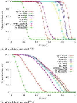
Figures6 and7show the baseline results for FPPS and FPNS respectively (the graphs are best viewed online in colour). Table5summarises these results using the weighted schedulability measure (Bastoni et al.2010).
Additional experimental results showing how this measure varies with the number of tasks and with the memory latency are given in the next subsection on weighted schedulability.
Table 4 WCETs from the Mälardalen and EEMBC benchmarks used for evaluation
Name Cwb Cwt Cwt/Cwb Cnc Cnc/Cwb
cnt 9325 13485 1.44 24565 2.63
compress 10673 18713 1.75 43443 4.07
countneg 36180 57250 1.58 114340 3.16
crc 68889 133909 1.94 272859 3.96
expint 9268 15208 1.64 31098 3.35
fdct 7883 16793 2.13 38423 4.87
fir 8328 18998 2.28 43668 5.24
jfdctint 9711 18621 1.91 39181 4.03
loop3 14189 28729 2.02 57929 4.08
ludcmp 10058 15948 1.58 39668 3.94
minver 18976 30616 1.61 54746 2.88
ns 27464 37674 1.37 98634 3.59
nsichneu 18988 24458 1.28 66808 3.51
qurt 10473 16003 1.52 23573 2.25
select 8981 17031 1.89 30331 3.37
sqrt 27667 40537 1.46 59117 2.13
statemate 64638 195778 3.02 581908 9.00
a2time 12655 22975 1.81 53815 4.25
aifirf 44898 86768 1.93 181698 4.04
basefp 50491 92221 1.82 213771 4.23
canrdr 32641 65211 1.99 156611 4.79
iirflt 29995 56995 1.90 127605 4.25
pntrch 23887 43137 1.80 109257 4.57
puwmod 48782 97072 1.98 239752 4.91
rspeed 10913 21393 1.96 51713 4.73
tblook 12533 25493 2.03 58813 4.69
the stand-alone WCETs for write-back caches, but without any cost for write backs. This line upper bounds the performance of any sound analysis for write-back caches, and thus gives an indication of the precision of the analyses introduced in this paper. The line write-back flush corresponds to a pessimistic analysis for write-back caches. In the case of FPNS, this analysis assumes that the entire cache is dirty and is flushed (written back) at the start of each task. To account for this, the WCET for each task is increased byN·W BT, whereN is the number of caches lines (e.g. 512) and
Fig. 6 Number of schedulable task sets (FPPS)
[image:27.439.86.352.54.408.2]Fig. 7 Number of schedulable task sets (FPNS)
Table 5 Weighted schedulability measure for FPNS and FPPS
Approach FPPS FPNS
Write-back (upper bound) 0.793458 0.445750
Combined 0.693003 0.412270
(F)DCB-Union 0.692087 0.411087 ECB-Union 0.672489 0.396159
(F)DCB-Only 0.561542 0.396159
ECB-Only 0.581876 0.365523 Write-back (flush) 0.304987 0.305039
Write-through 0.249231 0.112666
[image:27.439.166.389.425.561.2]by 2N·W BT. The results forwrite-back flushlower bound any useful analysis for a write-back cache.
For preemptive scheduling, inall cases, we include the cost of additional cache misses due to CRPD using the UCB-Union approach (Altmeyer et al.2012).
The results shown in Figs.6and7indicate that the guaranteed performance obtained for write-back caches using the analyses introduced in this paper exceeds that which can be obtained for write-through caches. The new methods also provide a substantial improvement over the pessimistic write-back flush analysis, which in turn has an advantage over analysis for write-through caches. This shows that the gain from using a write-back cache comes from a combination of reduced WCETs and accurate analysis. Further, theupper boundline indicates that the combined approaches used to anal-yse write-back cache offer a high degree of precision.
In Figs.6and7the ECB-Union approaches are outperformed by DCB-Union and FDCB-Union respectively. We note that this is not always the case as shown by the worked example in Sects.5.4and4.3. In our experiments, the performance of the DCB-Union approach for FPPS and the FDCB-Union approach for FPNS is close to that of the associated combined approach. The reason for this is the relatively weak performance of the ECB-Union approach in each case. This occurs because the sets of ECBs for the benchmark tasks are substantially larger than the sets of DCBs and FDCBs. This degrades the relative performance of the ECB-Union approaches, particularly for low priority tasks which are the most critical to task set schedulability. (For a low priority task, the union of ECBs over all higher priority tasks may well cover all of the cache).
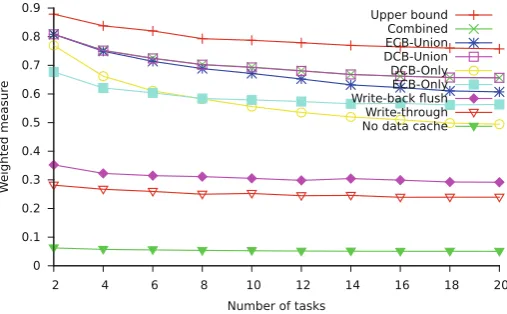
7.1 Weighted schedulability
The weighted schedulability measureWy(p)for a schedulability testyand parameter p, combines results for all task sets generated for a set of equally spaced utilization levels (e.g. from 0.025 to 0.975 in steps of 0.025). LetSy(τ,p)be the binary result (1
or 0) of schedulability testyfor a task setτ assuming parameterp.
Wy(p)=
∀τ
u(τ )·Sy(τ,p) /
∀τ
u(τ ) (29)
whereu(τ )is the utilization of task setτ. Weighting the results by task set utilization reflects the higher value placed on being able to schedule higher utilization task sets. Figures8and9show how the weighted schedulability measure varies with task set size for FPPS and FPNS respectively. With preemptive scheduling, the relative performance of the different approaches remains consistent, with an overall gradual decline in schedulability as the number of tasks increases. This is due to an increase in the number of tasks increasing the number of preemptions and to some degree also their cost. (With FPPS, it is also simply harder to schedule task sets with increasing numbers of tasks, even without considering overheads).
Fig. 8 Weighted schedulability versus number of tasks (FPPS)
Fig. 9 Weighted schedulability versus number of tasks (FPNS)
with a write-back cache; however, at the very low level of schedulability achieved by write-through cache and no cache, schedulability is more dependent on a random choice of tasks with similar WCETs and hence similar deadlines, which avoid the long task problem. This becomes rarer with more tasks counteracting the previous effect.
[image:29.439.92.346.55.212.2] [image:29.439.92.348.244.397.2]Fig. 10 Weighted schedulability versus memory latency (FPPS)
Fig. 11 Weighted schedulability versus memory latency(FPNS)
(e.g. 20 vs. 5 cycles, 40 vs. 10 cycles, or 80 vs. 20 cycles). For FPNS, where long task execution times have an increased impact on schedulability, the difference was even more stark, with the guaranteed performance obtained with a write-back cache with a memory delay of 40 cycles similar to that with a write-through cache with a delay of 5 cycles.
8 Write buffers
In this section, we discusswrite buffersand their use, predominantly in improving the performance of write-through caches. At the end of the section we discuss the use of write buffers for write-back caches.
[image:30.439.91.347.237.393.2]can, to a large extent, be remedied via the use of awrite buffer. A write buffer is a small buffer that operates between the cache and main memory. It holds data that is waiting to be written to memory. When a write occurs, the address and data (block) are placed in the write buffer. This allows the processor to continue with subsequent instructions, while the write to memory occurs in parallel via the write buffer.
Write buffers are characterized by adepth(indicating the number of entries), and awidth(which is typically the same as a cache line), as well as the policies defining their operation. These policies include: (i) thelocal-hazardpolicy, which determines what happens when a read access occurs to an address that is currently in the write buffer; (ii) thecoalescence policy, which determines what happens when a write access occurs to an address that is currently in the write buffer, and finally (iii) theretirement policy, which determines when write buffer entries are retired, i.e. written to memory. We discuss these policies in more detail below. (The interested reader is also referred to the work of Skadron and Clark (1997), which discusses write buffer design from the perspective of improving average-case performance).
8.1 Local hazard policy
Care is needed in the design of a write buffer, since a naive design could potentially result in data inconsistency, termed alocal hazard, as follows: If a read occurs which is a cache miss, but the data is in the write buffer waiting to be written to memory, then reading from memory could result in an inconsistent value being obtained. To avoid this hazard there are two possible options that we consider (i)read from the write bufferor (ii)full flush of the write bufferand then read from memory. (More complex schemes are possible, such as flushing the write buffer only as far as necessary to write the required data to memory, or flushing only the specific item. They are not considered here).
8.2 Coalescence policy
Entries in a write buffer consist of an address and a block of data. The latter is typically the same size as a cache line. When a write occurs and there are no entries in the write buffer, then the block of data is copied to the write buffer and the specific word that is being written is marked as valid via a flag bit. The flag bit indicates that the word should later be written to memory.
If a write occurs to an address that is already in an entry in the write buffer then it could potentially be coalesced. In this case the entry containing the address is found in the buffer and the appropriate word of data is updated and marked as valid. We refer to this mechanism aswrite merge. Merging writes in this way has the advantage that it enables multiple writes to the same address or to the same block to be coalesced, resulting in fewer writes to memory. The write-merge mechanism has similarities to a write-back cache, in that it takes advantage of the spacial locality of writes. Merging writes also makes better use of the limited capacity of the write buffer.