Escaping Local Optima Using Crossover with
Emergent Diversity
Duc-Cuong Dang, Tobias Friedrich, Timo K¨otzing, Martin S. Krejca, Per Kristian Lehre, Pietro S. Oliveto,
Dirk Sudholt, Andrew M. Sutton
Abstract—Population diversity is essential for avoiding pre-mature convergence in Genetic Algorithms and for the effective use of crossover. Yet the dynamics of how diversity emerges in populations are not well understood. We use rigorous run time analysis to gain insight into population dynamics and Genetic Algorithm performance for the (µ+1) Genetic Algorithm and the
Jump test function. We show that the interplay of crossover followed by mutation may serve as a catalyst leading to a sudden burst of diversity. This leads to significant improvements of the expected optimisation time compared to mutation-only algorithms like the (1+1) Evolutionary Algorithm. Moreover, increasing the mutation rate by an arbitrarily small constant factor can facilitate the generation of diversity, leading to even larger speedups. Experiments were conducted to complement our theoretical findings and further highlight the benefits of crossover on the function class.
Index Terms—Genetic algorithms, recombination, diversity, run time analysis, theory
I. INTRODUCTION
Genetic Algorithms (GAs) are powerful general-purpose optimisers that perform surprisingly well in many applications, including those where the problem is not well understood to apply a tailored algorithm. Their wide-spread success is based on a number of factors: using populations to diversify search, using mutation to generate novel solutions, and using crossover to combine features of good solutions.
Pr¨ugel-Bennett [29] gives several reasons for the success of populations and crossover. Crossover can combine building blocks of good solutions and help to focus the search on bits where parents disagree [29]. For both tasks, the population needs to be diverse enough; without sufficient diversity in the population, crossover is not effective. A common problem in the application of GAs is the loss of diversity when the population converges to copies of the same search point, often calledpremature convergence. Understanding how populations gain and lose diversity during the course of the optimisation is vital for understanding the working principles of GAs and for tuning the design of GAs to get the best possible performance. Rigorous run time analysis has emerged as a powerful theory that has provided many insights into the performance of GAs [1], [5], [17], [24], [26], [27], including the benefit
D.-C. Dang is with the ASAP Research Group at the School of Computer Science, University of Nottingham, United Kingdom.
P. K. Lehre is with the School of Computer Science, University of Birmingham, United Kingdom.
T. Friedrich, T. K¨otzing, M. S. Krejca and A. M. Sutton are with the Chair of Algorithm Engineering, Hasso Plattner Institute, Potsdam, Germany.
P. S. Oliveto and D. Sudholt are with the Department of Computer Science, University of Sheffield, United Kingdom.
of crossover [9], [18], [20], [21], [25], [31]. It has guided algorithm design, including the discovery of new variants of GAs such as the (1+(λ,λ)) GA [8], which has shown very good performance across a range of hard problems [14].
However, understanding population diversity and crossover has proved elusive. The first example function where crossover was proven to be beneficial is calledJumpk. In this problem, GAs have to overcome a fitness valley such that all local optima have Hamming distance k to the global optimum. Jansen and Wegener [18] showed that, while mutation-only algorithms such as the (1+1) EA require expected time Θ(nk), a simple (µ+1) GA with crossover only needs time O µn2k3+ 4k/pc
. This time is O 4k/pc
for large k, and hence significantly faster than mutation-only GAs. However, their analysis requires an unrealistically small crossover prob-abilitypc≤1/(ckn)for a large constant c >0.
K¨otzing, Sudholt, and Theile [20] later refined these re-sults towards a crossover probability pc ≤ k/n, which is
still unrealistically small. Both approaches focus on creating diversity through a sequence of lucky mutations, relying on crossover to create the optimum, once sufficient diversity has been created. Their arguments break down if crossover is applied frequently. Hence, these analyses do not reflect the typical behaviour in GA populations with constant crossover probabilitiespc = Θ(1)as used in practice [22].
Lehre and Yao analysed the run time of the (µ+1) GA with deterministic crowding for arbitrary crossover rates pc > 0,
showing exponential run time gaps between the case pc = 0
and pc > 0 [21]. The gain in performance in that analysis
stems from the ability of a diverse population to optimise mul-tiple, separated paths in parallel using a diversity-preservation mechanism. Similar results have been also shown for instances of the vertex cover problem by generating diversity, either through deterministic crowding [25] or through island models [23]. Recently in [7], we have shown that a small change to the tie-breaking rule of the (µ+1) GA to introduce many common principles of preserving diversity can lead to a size-able advantage on the expected optimisation time ofJumpk function. The results hold for realistic crossover probabilities
pc = 1−Ω(1). In the present paper, we will consider a very
different effect.
equilibrium, where the state of a population is described by the frequency of alleles [3].
For the maximum crossover probability pc = 1, we show
that on Jumpk diversity emerges naturally in a population: the interplay of crossover, followed by mutation, can serve as a catalyst for creating a diverse range of search points out of few different individuals. This naturally emerging diversity allows proving a speedup of order n/logn for k ≥ 3 and standard mutation rate pm= 1/n compared to mutation-only
algorithms such as the (1+1) EA. Increasing the mutation rate topm= (1+δ)/nfor an arbitrarily small constantδ >0, leads
to a speedup of order n. The detail can be seen in Table I. Both operators are proven to be vital: mutation requires Θ(nk) expected iterations to hit the optimum from a local optimum. Also using crossover on its own does not help much. As shown in [20, Theorem 8], using only crossover withpc= Ω(1)but no mutation following crossover, diversity
reduces quickly, leading to inefficient running times for small population sizes (µ= O(logn)).
All our analyses are based on observing the dynamic behaviour of the size of the largest species, referring to a collection of identical genotypes as species. A population con-tains no diversity when only one species is present. However, mutation can create further species, and then the combination of crossover and mutation is able to rapidly create further species in a highly stochastic process. This diversity can then be exploited to find the global optimum onJumpk efficiently. A higher mutation rate facilitates the generation of new species and leads to better performance, with respect to rigorous upper run time bounds and empirical performance.
Using Jumpk as a case study, our analyses shed light on how diversity emerges in populations and how to facilitate the emergence of diversity by tuning the mutation rate. The general proof strategy we take is as follows. We characterise the size of the largest species as a stochastic process and calculate the transition probabilities of this process taking into account both mutation and crossover. We prove that the size of the largest species is described either by an almost-fair random walk (for standard mutation rates), or by an unfair random walk that is biased toward increased diversity (for higher mutation rates). This ultimately allows us to bound the expected time until sufficient diversity is present in the population to perform a crossover that successfully generates the global optimum. Our main results are stated in Theorems 6 and 10, which yield our run time bounds under the assumed conditions. Critical lemmas are Lemma 2, which estimates the time until the entire population has reached the plateau using the method of fitness-based partitions, and Lemma 4, which bounds the transition probabilities for the random walk dynamics of the size of the largest species. The proof of Lemma 4 is carried out by a careful analysis of the different events that can occur while the entire population resides on the plateau.
This work is based upon our preliminary study published in [6]. Here we extend the analysis to higher mutation rates, leading to the surprising conclusion that increasing the mutation rates leads to smaller run time bounds, compared to the standard mutation rate 1/n. Furthermore, the analysis
0 1 2 3 4 5 6 7 8 9 10
A1 A2 A3 A4 A5 A6 A7 A8 A9
A10
plateau
gap optimum
|x|1
Jump
3
(
x
[image:2.612.317.557.55.192.2])
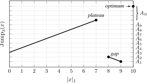
Figure 1. Illustration of the Jumpkfitness function for the casen= 10and
k= 3, including the levelsA1, . . . , A10defined in the proof of Lemma 2.
of standard mutation rates in [6] was restricted to very short jumps, k = O(1). Here we generalise the results to a much larger class of Jumpk functions, only requiring k = o(n). Experiments were conducted to complement the theoretical re-sults and further highlight the benefits of combining crossover with mutation. In fact, the experimental results showed that the setting of high mutation rate can be as competitive as using specific diversity mechanisms from [7].
II. PRELIMINARIES
TheJumpk:{0,1}n→
N class of pseudo-Boolean fitness functions was originally introduced by Jansen and Wegener [18]. The function value increases with the number of 1-bits in the bit string until a plateau of local optima is reached, consisting of all points with n−k 1-bits. However, its only global optimum is the all-ones string1n. Between the plateau and the global optimum, there is a valley of bad fitness, which we call the gap of length k, and the algorithm has to jump over this gap to optimise the function.
The function is formally defined as Jumpk(x) =
(
k+|x|1 if|x|1=nor |x|1≤n−k, n− |x|1 otherwise,
where|x|1=P
n
i=1xi is the number of 1-bits inx. Figure 1 illustrates the function, with the number of 1-bits on the horizontal axis, and the function value on the vertical axis.
We will analyse the performance of a standard steady-state (µ+1) GA [18] using uniform crossover (i.e., each bit of the offspring is chosen uniformly at random from one of the parents) and standard bit mutation (i.e., each bit is flipped with probability pm). The algorithm uses a population of µ
individuals. In each generation, a new individual is created. With probability pc, it is created by selecting two parents
from the population uniformly at random, crossing them over, and then applying mutation to the resulting offspring. With probability 1−pc instead, one single individual is selected
and only mutation is applied. The generation is concluded by removing the worst individual from the population and breaking ties uniformly at random. Algorithm 1 shows the pseudocode for the (µ+1) GA. Note thatP is a multiset.
Table I
SOME EXAMPLES OF RUN TIME BOUNDS WE OBTAIN FOR THE(µ+1) GAONJumpk.
Algorithmic setting µ pc pm Problem
k= 2 k= 4 k= o(n)
Standard mutation, Thm. 6 Θ
√
n √
logn
1 1/n O√n1.5
logn
O√n3.5 logn
On√k−0.5 logn
Θ(n) 1 1/n O n2logn
O n3logn
O nk−1logn High mutation, Thm. 10 Θ(logn) 1 (1 +δ)/n O(nlognlog logn) O n3
On√klognlog logn+nk−1
Algorithm 1: (µ+1) GA
1 P ←µ individuals, uniformly at random from{0,1}n; 2 while 1n∈/ P do
3 Choosep∈[0,1]uniformly at random; 4 if p≤pc then
5 Choosex, y∈P uniformly at random; 6 z←mutate(crossover(x, y));
7 else
8 Choosex∈P uniformly at random; 9 z←mutate(x, pm);
10 P ←P∪ {z};
11 Remove one element from P with lowest fitness, breaking ties uniformly at random;
local optima, the so-called plateau. That is because under the right condition the population diversity will emerge during this stage. Then after sufficient progress is made in diversity, crossover and mutation can work together on the plateau to create an optimal solution in o nktime. This is captured by Lemma 14, which will be presented later in the paper.
For the sake of completeness, in the next section, we provide the time bounds for the population to reach the plateau for the general setting of pc= Ω(1). This covers the case ofpc= 1
which we will actually focus on in the main results. III. TIME TO PLATEAU
In the setting of pc = Ω(1), we direct the attention to the
steps that crossover occurs. We make use of the following general result, which provides an upper bound on the expected time for the (µ+1) GA to reach some regionAmof the search space. Here we consider afitness-basedpartition (see [17] for a formal definition) into levels(Ai)i∈[m] (thus,Amis the last level) and define A≥j :=S
m i=jAi.
Theorem 1. Let (Ai)i∈[m] be a fitness-based partition of the search space into m ∈ N levels. If there exist parameters ε, s1, . . . , sm−1∈(0,1]such that for allj∈[m−1]
1) minx∈A≥j,y∈A≥j+1
Pr(mutate(crossover(x, y))∈A≥j+1)≥εand 2) minx,y∈AjPr(mutate(crossover(x, y))∈A≥j+1)≥sj then the expected number of iterations until the entire pop-ulation of the (µ+1) GA with pc = Ω(1) is in Am is O(µm/ε) log(µ) +Pm−1
j=1 1/sj
.
Proof. The proof follows [5], but we avoid a detailed drift analysis because the algorithm is elitist, i.e., the maximum fitness in the population does not decrease. Let the current levelbe the smallesti∈[m]such that the population contains less thanµ/2individuals inA≥i+1. By definition, there are at
least µ/2 individuals inA≥j, wherej is the current level. Since the algorithm is elitist, the number of individuals in
A≥j is non-decreasing for any j∈[m]. For an upper bound, we ignore any improvements where mutation only is used (i.e., lines 8 and 9 in Alg. 1).
Assume that there are i individuals in A≥j+1, hence 0 ≤ i < µ/2. Ifi= 0, then an individual inA≥j+1can be created
by selecting two individuals fromAj, crossing them over, and mutating them such that the offspring is in A≥j+1 and an
individual not in A≥j+1 is removed. The probability of this
event is at least pcsj/4, where the 1/4 is the probability of selecting two individuals fromAj, which contains at leastµ/2 individuals.
If 0< i < µ/2, then the number of individuals in A≥j+1
can be increased by selecting an individual in A≥j and an individual inA≥j+1, crossing them over, and mutating them
such that the offspring is inA≥j+1and one of theµ−i > µ/2
individuals not inA≥j+1 is removed. This event occurs with
probability at least(pc/2)(i/µ)ε.
The expected time to increase the number of individuals in A≥j+1 from 0 to µ/2, i.e., to increase the current level
by at least one, is4/(pcsj) + 2µ/(pcε)P
µ/2
i=11/i. Hence, the
expected time until at least half of the population is inAm is O(µm/ε) log(µ) +Pm−1
j=1 1/sj
.
We now consider the time to remove individuals from the lowest fitness level in the population, assuming that at least half of the population has reached the last levelAm.Assume that there are 0 < i0 < µ/2 individuals in the lowest level
j < m. The number of individuals in level j can be reduced by crossing over an individual in leveljand one of the at least
µ/2 individuals in levelm, and mutating the offspring so that it belongs to A≥j+1. By condition 1, this event occurs with
probability at leastpc(ε/2)(i0/µ). Hence, the expected time to
remove all individuals from the lowest leveljis no more than (2/pcε)µP
µ/2
i0=11/i0 = O((µ/ε) logµ). The expected time until all individuals in fitness levels lower thanm have been removed is thereforeO(µ(m/ε) logµ).
Lemma 2. Consider the (µ+1) GA optimising Jumpk with pc = Ω(1) and pm = Θ(1/n). Then the expected time until either the optimum has been found or the entire population is on the plateau isOn√k(µlogµ+ logn).
Proof. We divide the search space into m:=nfitness levels with the partition
Aj :=
x∈ {0,1}n| |x|
1=n−j if1≤j < k,
x∈ {0,1}n| |x|
1=j−k ifk≤j < n,
x∈ {0,1}n| |x|
1∈ {n−k, n} ifj =n.
We call any search pointx∈ {0,1}nwithn−k <|x|
1< n
a gap-point. Gap-points have worse fitness than any other search point, hence once there are no gap-points left in the population, the algorithm will not accept any further gap-points. We can therefore divide the run into two phases, with phase 1 lasting as long as the population contains at least one gap-individual, followed by phase 2, which lasts until the optimum or a plateau individual has been found.
We bound the duration of the two phases by applying Theorem 1 twice, once for each of the two phases.
We start by estimating the expected duration of phase 2 using Theorem 1 with respect to levels Ak to level An. We claim that the probability of producing a gap-point by crossing over two individuals x∈A≥j andy ∈A≥j+1 withk≤j < n+ 1satisfies
Pr(n−k <|crossover(x, y)|1< n)<
1 2−
1
4√k . (1)
To see why this claim holds, we first argue that the probability of producing a gap-point is highest when both parents, x and y, have n−k 1-bits. More formally, obtain
x0 by flipping an arbitrary 0-bit in x, and y0 by flipping an arbitrary 0-bit in y. Then, we have the stochastic dominance relationships |crossover(x, y)|1 |crossover(x0, y)|1 and |crossover(x, y)|1 |crossover(x, y0)|1. By repeating this
ar-gument, we obtain |crossover(x, y)|1 |crossover(x00, y00)|1
for two bit strings x00 and y00 with |x00|1 = |y00|1 = n−k.
The probability of obtaining a search point with exactly k
0-bits when crossing over two bit strings with k 0-bits each is minimised when all positions of the 0-bits in the two bit strings differ. Hence, for bit strings x00 and y00, we have by
Stirling’s approximation the lower bound Pr(|crossover(x00, y00)|1=n−k)>
2k k
·2−2k
≥ 2
2k
2√k·2
−2k= 1 2√k .
Uniform crossover of the bit strings x00 and y00 creates two bit strings u00 andv00, and returns eitheru00 or v00 with equal probability. We then have
2(n−k) =|x00|1+|y00|1=|u00|1+|v00|1 . (2)
The event |u00|1 =|v00|1 =n−k therefore equals the event |crossover(x00, y00)|1 = n−k. Otherwise, in the event that |u00|
1 6= |v00|1, we assume without loss of generality that
|u00|1 > |v00|1. We must then have |v00|1 < n−k < |u00|1
because
2|v00|1<|u00|1+|v00|1= 2(n−k) =|u00|1+|v00|1<2|u00|1.
The claimed inequality (1) now follows, because Pr(n >|crossover(x00, y00)|1> n−k)
<Pr(|crossover(x00, y00)|1> n−k)
=1 2Pr(|u
00|
16=|v00|1)
=1
2(1−Pr(|u
00|
1=|v00|1))
=1
2(1−Pr(|crossover(x
00, y00)|
1=n−k))
≤1 2 −
1
4√k .
We now show that condition 1 of Theorem 1 holds for the parameter ε := (1−pm)n/(4
√
k) = Θ(1/√k). Assume that x ∈A≥k+j and y ∈ A≥k+j+1 for j ≥0. By the same
arguments as above,
2j+ 1≤ |x|1+|y|1=|u|1+|v|1≤2|u|1 ,
where we assume without loss of generality that |u|1 ≥ |v|1.
A crossover betweenxandytherefore produces two offspring
uandv where|u|1≥j+ 1, hence
Pr(j+ 1≤ |crossover(x, y)|1)≥1/2. (3)
Combining (1) and (3) now yields Pr(crossover(x, y)∈A≥k+j+1)
= Pr(j+ 1≤ |crossover(x, y)|1)
−Pr(n−k <|crossover(x, y)|1< n)
≥ 1
4√k .
Finally, with probability(1−pm)n, none of the bits are flipped
during mutation, which implies
Pr(mutate(crossover(x, y))∈A≥k+j+1)≥ε .
We now show that condition 2 of Theorem 1 holds. Assume that x, y ∈ Aj+k for j ≥ 0. Then, following the same arguments as above
Pr(crossover(x, y)∈A≥k+j)≥ 1
4√k .
The probability that the mutation operator flips at least one of the n−j 0-bits, and no other bits, is at least(n−j)pm(1− pm)n−1. Hence, we can use the parametersj := (n−j)pm(1− pm)n−1/(4
√
k) = Θ((n−j)/(n√k)).
We have shown that both condition 1 and condition 2 hold during phase 2, which by Theorem 1 implies that the expected duration of phase 2 isOn√k(µlogµ+ logn).
generation (t)
mutation
param.
(
χ
[image:5.612.53.295.59.194.2]) Average size of the largestspecies on the plateau
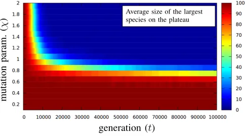
Figure 2. Empirical investigation of diversity on the plateau.
expectation duration of phase 1 and phase 2, and the theorem follows.
In the following sections, we first show that once the plateau ofJumpkhas been reached by the (µ+1) GA withpc = 1, the
population diversity can emerge naturally from the interaction between crossover and mutation. Based on such a result on the population dynamics, bounds on the expected optimisation time of the function class are then deduced for two different settings of the algorithm: standard and high mutation rates.
IV. POPULATION DYNAMICS
Assume that the algorithm has reached a population where all individuals are identical and on the plateau, i. e., the less diverse setting. We refer to identical individuals as a species, hence, in this case, there is only one species. Eventually, a mutation will create a different search point on the plateau, leading to the creation of a new species. Both species may shrink or grow in size, and there is a chance that the new species will disappear and that we return to one species only. However, the existence of two species also serves as a catalyst for creating further species in the following sense. Say two parents0001111111and0010111111are recombined, then crossover has a good chance of creating an individual with
n−k+ 1 1s, e.g.,0011111111. Then mutation has a constant probability of flipping any of then−k−1unrelated 1-bits to 0, leading to a new species, e. g.,0011111011. This may lead to a sudden burst of diversity in the population.
To further investigate these dynamics, we set up a prelim-inary experiment for n = 500, k = 3, with population size
µ = 100 and mutation parameter χ from [0.1,0.2, . . .2.0]. Since we are only interested in the dynamics on the plateau, the optimum is always rejected and the population is initialised with copies of a single plateau solution.100independent runs are repeated for each setting, and as an indicator of diversity, the size of the largest species is recorded for the first 105
iterations of each run. Figure 2 illustrates the obtained result. Clearly, we see that new species can emerge from time to time and more importantly if the mutation rate χ/nis sufficiently large then a diverse population can be maintained (size of the largest species remains close to 1) after some time.
The above simulation indicates that the mutation rate and the size of the largest species are important factors for
describ-ing the population diversity. With a large enough mutation rate, the size of the largest species can perform a random walk biased towards a reduction of its value. Once its size has decreased significantly from its maximum µ, there is a good chance for recombining two parents from different species. This helps in finding the global optimum, as crossover can increase the number of 1s in the offspring, compared to its parents, such that fewer bits need to be flipped by mutation to reach the optimum. This is formalised in the following lemma. Lemma 3. The probability that the global optimum is con-structed by a uniform crossover of two parents on the plateau having Hamming distance2d, followed by mutation, is
2d
X
i=0
2d i
1 22dnk+d−i
1−1
n
n−k−d+i
(4)
≥ 1
22dnk−d
1−1
n
n−k+d
. (5)
Proof. For a pair of search points on the plateau with Ham-ming distance 2d, both parents have d1s among the 2d bits that differ between parents, andn−k−d1s outside this area. Assume that crossover setsiout of these2dbits to 1, which happens with probability 2id·2−2d. Then mutation needs to flip the remainingk+d−i0s to 1. The probability that such a pair creates the optimum is hence
2d
X
i=0 2d
i
1
22dnk+d−i
1−1
n
n−k−d+i .
The second bound is obtained by ignoring summands i <2d
for the inner sum.
Note that even a Hamming distance of 2, i.e., d = 1, leads to a probability ofΩ(n−k+1), provided that such parents
are selected for reproduction. The probability is by a factor of n larger than the probabilityΘ(n−k)of mutation without crossover reaching the optimum from the plateau.
We will show that this effect leads to a speedup of nearly
nfor the (µ+1) GA, compared to the expected time ofΘ(nk) for the (1+1) EA [10] and other EAs only using mutation.
The idea behind the analysis is to investigate the random walk underlying the size of the largest species. We bound the expected time for this size to decrease toµ/2and then argue that the (µ+1) GA is likely to spend a good amount of time with a population of good diversity, where the probability of creating the optimum in every generation isΩ(n−k+1)due to
the chance of recombining parents of Hamming distance at least 2.
In the following, we refer toY(t)as the size of the largest species in the population at time t. Define
p+(y) := Pr(Y(t+ 1)−Y(t) = 1|Y(t) =y),
p−(y) := Pr(Y(t+ 1)−Y(t) =−1|Y(t) =y),
i.e.,p+(y)is the probability that the size of the largest species
increases fromytoy+ 1, andp−(y)is the probability that it
decreases fromy toy−1.
than 2 are selected for recombination (this case will be treated later in Lemma 5). We formulate the lemma for arbitrary mutation rates χ/n = Θ(1/n) and restrict our attention to sizes Y(t) ≥µ/2 as we are only interested in the expected time for the size to decrease toµ/2.
Lemma 4. For every population on the plateau of Jumpk
for k= o(n), the following holds. Either the (µ+1) GA with mutation rate χ/n = Θ(1/n) performs a crossover of two parents whose Hamming distance is larger than 2, or the sizeY(t)of the largest species changes according to transition probabilitiesp−(µ) = Ω(k/n)and, forµ/2≤y < µ,
p+(y)≤
y(µ−y)(µ+y) 2µ2(µ+ 1)
1−χ
n n
+ O
(µ−y)2
µ2n
,
p−(y)≥
y(µ−y)(µ+χy) 2µ2(µ+ 1)
1−χ
n n
.
Proof. We call an individual belonging to the current largest species ay individual and all the others non-y individuals. In each generation, there is either no change, or one individual is added to the population and one individual chosen uniformly at random is removed from the population. In order to increase the number ofy individuals, it is necessary that ay individual is added to the population and a non-y individual is removed from the population. Analogously, in order to decrease the number ofyindividuals, it is necessary that a non-yindividual is added to the population and ayindividual is removed from the population.
Given that Y(t) = y, let p(y) be the probability that a y
individual is created at timet+1, andq(y)the probability that a non-y individual is created. Since all considered individuals are on the plateau, the individual for deletion is selected uniformly at random. Multiplying by the survival probabilities we have
p−(y) =q(y)
y µ+ 1
and (6)
p+(y) :=p(y)
1−y+ 1
µ+ 1
=p(y)
µ−y
µ+ 1
. (7) We now estimate an upper bound onp(y). We may assume that the Hamming distance between parents is at most 2 as otherwise there is nothing to prove. A y individual can be created in the following three ways:
• Two y individuals are selected. Crossing over two y
individuals produces anotheryindividual, which survives mutation if no bits are flipped, i.e., with probability (1−χ/n)n.
• One y individual and one non-y individual are selected.
The crossover operator produces ayindividual with prob-ability 1/4(as the individuals have Hamming distance 2 by assumption), and mutation does not flip any bits with probability(1−χ/n)n. If the crossover operator does not produce a y individual, then, to produce a y individual, at least one specific bit-position must be mutated, which occurs with probability O(1/n). The overall probability is hence (1/4)(1−χ/n)n+ O(1/n).
• Two non-yindividuals are selected. These two individuals are either identical or have Hamming distance 2(i.e., by
assumption). In the first case, they both have one of the
k0-bit positions of ay individual set to1. In the second case, they either both have one of the k 0-bit positions of a y individual set to 1, or they both have one of the
n−k 1-bit positions set to 0. In both cases, crossover cannot change the value of such a bit. Thus, at least one specific bit-position must be flipped, which occurs with probabilityO(1/n).
Taking into account the probabilities of the three selection events above, the probability of producing a y individual is
p(y) =
y µ
2
1−χ
n n + 2 y µ
1−y
µ · · 1 4
1−χ
n n + O 1 n
+(µ−y)
2
µ2 O
1
n
=1−χ
n
ny
µ
y
µ+ µ−y
2µ
+
+ O
y(µ−y) µ2 ·
1
n
+ O
(µ−y)2 µ2 ·
1
n
= y(µ+y) 2µ2
1−χ
n n
+ O
µ−y
µ ·
1
n
.
We then estimate a lower bound onq(y). In the case where
y=µ, a non-y individual can be added to the population if
• twoy individuals are selected and the mutation operator flips one of thek0-bits and one of then−k1-bits. This event occurs with probability
q(µ) =k(n−k)χ
n
2
1−χ
n n−2
(8) = Ω k n− k2 n2 = Ω k n , (9)
where we used that k= o(n)in the last equality.
In the other case, wherey < µ, a non-y individual can be added to the population in the following two ways:
• A y individual and a non-y individual are selected.
Crossover produces a copy of the non-y individual with probability 1/4, which is unchanged by mutation with probability (1−χ/n)n. Secondly, with probability1/4, crossover produces an individual with k − 1 0-bits. Mutation then creates a non-y individual by flipping a single of then−k1-bit positions that do not lead to re-creatingy. Thirdly, again with probability1/4, crossover produces an individual with k+ 1 0-bits and mutation then creates a non-y individual by flipping a single of
k 1-bits that do not lead back to y. The above three events, conditional on selecting ayindividual and a
non-y individual, lead to a total probability of 1
4 ·
1−χ
n n
+1
4 ·(n−k)·
χ n
1−χ
n n−1
+1 4 ·k·
χ n
1−χ
n n−1
≥χ+ 1 4 ·
1−χ
n n
.
at least 1/2, which mutation does not destroy with probability(1−χ/n)n.
Assuming that µ/2 ≤y < µ and n is sufficiently large, the probability of adding a non-y individual is
q(y)≥2
y
µ
1−y
µ
·χ+ 1 4
1−χ
n n
+1 2
1−y
µ
2
1−χ
n n
= (µ−y)(µ+χy) 2µ2
1−χ
n n
.
Plugging p(y)andq(y)into equations (6) and (7), we get
p−(y)≥
(µ−y)(µ+χy)
2µ2
1−χ
n
n y
µ+ 1
=(µ−y)(µ+χy)y 2µ2(µ+ 1)
1−χ
n n
.
And we also have
p+(y) =
y(µ+y)
2µ2
1−χ
n n + O µ −y µ · 1 n µ −y µ+ 1
= (µ
2−y2)y
2µ2(µ+ 1)
1−χ
n n
+ O
(µ
−y)2 µ2n
.
Steps where crossover recombines two parents with larger Hamming distance were excluded from Lemma 4 as they require different arguments. The following lemma shows that conditional transition probabilities in this case are favourable in that the size of the largest species is more likely to decrease than to increase.
Lemma 5. Assume that y≥µ/2 and that the (µ+1) GA on
Jumpk with k = o(n) and mutation rate χ/n = Θ(1/n)
selects two individuals on the plateau with Hamming distance larger than 2, then for conditional transition probabilities p∗−(y)andp∗+(y)for decreasing or increasing the size of the largest species, p∗
−(y)≥2p∗+(y).
Proof. Assume that the population contains two individualsx
andzwith Hamming distance2`≤2k, where`≥2. Without loss of generality, let us assume that they differ in the first2`
bit positions.
First assume that the individual y representing the largest species has`0-bits in the first2`positions. Then ayindividual may be produced by creating the ` 0-bits and ` 1-bits in the exact positions by crossover and no followed mutation. Alternatively, at least1exact bit has to be flipped by mutation. Then the probability of producing a y individual fromxand
z and replacing a non-y individual with y is less than
p∗+(y)≤
"
1
2
2`
1−χ
n n
+ O
1
n
#µ−y
µ
≤
1
2
2`+1
1−χ
n n + O 1 n .
On the other hand, the probability of producing an individual on the plateau different fromy and replacing ay individual is at least
p∗−(y)≥
2` ` −1 1 2 2`
1−χ
n
ny
µ
≥3
1
2
2`+1
1−χ
n n
≥2p∗+(y)
for sufficiently large n.
In the other case, assume that the individual y does not have ` 0-bits in the first 2` bit-positions. Then the mutation operator must flip at least one specific bit among the lastn−2`
positions to producey, which occurs with probabilityO(1/n). The probability to produce a non-yindividual on the plateau is lower bounded by the probability of the event that recombining
xandz produces a bitstring with exactlyk0-bits in the first 2` bit-positions, none of the bits are mutated, and a majority individual is replaced, i.e.,
p∗−(y)≥
2k
k
2−2k1−χ
n
ny
µ
≥2 2k−1 √
k 2
−2k1−χ
n
ny
µ
= Ω(1/
√
k).
where the inequality follows by Stirling’s inequality. Taking into account the assumptionk= o(n), it holds for sufficiently largenthat p∗−(y)≥2p∗+(y).
V. STANDARD MUTATION RATE
We first analyse the (µ+1) GA with the standard mutation rate of1/n, i.e.,χ= 1. We show that the diversity emerging in the (µ+1) GA leads to a speedup of nearlynfor the (µ+1) GA, compared to the expected time ofΘ(nk)for the (1+1) EA [10] and other EAs only using mutation.
Theorem 6. The expected optimisation time of the (µ+1) GA withpc= 1andµ≤κn, for some constantκ >0, onJumpk,
k= o(n), is
Oµn√klog(µ) +nk/µ+nk−1log(µ).
For k ≥ 3, the best speedup is of order Ω(n/logn) for
µ=κn. Fork= 2, the best speedup is of orderΩ(pn/logn) for µ= Θ(pn/logn).
Note that for mutation rate 1/n, the dominant terms in Lemma 4 are equal, hence the size of the largest species performs a fair random walk up to a bias resulting from small-order terms. This confirms our intuition from observing simulations. The following lemma formalises this fact: in steps where the sizeY(t)of the largest species changes, an almost fair random walk is performed.
Lemma 7. For the random walk induced by the size of the largest species, conditional on the current size y changing, for µ/2 < y < µ, the probability of increasing y is at most
1/2 + O(1/n), and the probability of decreasing it is at least
1/2−O(1/n).
sought probability is given byp+(y)/(p+(y) +p−(y)), which
is strictly increasing inp+(y). Lemma 5 states that whenever
the (µ+1) GA recombines two parents of Hamming distance larger than 2, the claim on conditional probabilities clearly follows. Hence we assume in the following that this does not happen.
Using the lower bound for p+(y) and the upper bound
for p−(y) from Lemma 4, with implicit constant c+ in the
asymptotic term for p+, we get p+(y)
p+(y) +p−(y)
≤
y(µ+y)(µ−y) 2µ2(µ+1) · 1−
1
n
n
+c+(µ−y)2
µ2n
y(µ+y)(µ−y)
µ2(µ+1) · 1−
1
n
n
+c+(µ−y)2
µ2n
=1 2 +
c+(µ−y)2
2µ2n
y(µ+y)(µ−y)
µ2(µ+1) · 1−
1
n
n
+c+(µ−y)2
µ2n
=1 2 +
c+(µ−y)
2µn y(µ+y)
µ(µ+1)· 1− 1
n
n
+c+(µ−y)
µn
,
where in the last step we multiplied the last fraction by
µ/(µ−y). Now the numerator isO(1/n). Sinceµ/2< y < µ, we have yµ((µµ++1)y) = Θ(1). Along with 1−1
n
n
= Θ(1)and c+(µ−y)
µn = O(1/n), the denominator simplifies to Θ(1) + O(1/n) = Θ(1). Hence the last fraction is O(1/n), proving the claim.
We use these transition probabilities to bound the expected time for the random walk to hitµ/2.
Lemma 8. Consider the random walk of Y(t), starting in state X0≥µ/2. Let T be the first hitting time of stateµ/2. If µ= O(n), thenE(T |X0) = O µn+µ2logµ
regardless ofX0.
Proof. Let Ei abbreviate E(T | X0 = i), then Eµ/2 = 0.
Since p−(µ) = Ω(1/n) by Lemma 4, the expected time to
leave state µtowards stateµ−1 is1/p−(µ) = O(n)and the
remaining time will be Eµ−1, thusEµ = O(n) +Eµ−1.
For µ/2 < y < µ, the probability of leaving state y is always (regardless of Hamming distances between species) bounded from below by the probability of selecting two y
individuals as parents, not flipping any bits during mutation, and choosing a non-y individual for replacement:
p+(y) +p−(y)≥ y2 µ2·
1−1
n
n
·µ−y
µ+ 1 ≥
µ−y
24µ ,
asy≥µ/2,µ+1≤3µ/2(sinceµ≥2), and(1−1/n)n≥1/4 forn≥2. Hence the expected time for leaving stateitowards either state i+ 1or statei−1 is at most24µ/(µ−i). Using conditional transition probabilities 1/2±δ for δ = O(1/n) according to Lemma 7, Ei is bounded as
Ei≤ 24µ µ−i+
1 2 −δ
Ei−1+
1 2 +δ
Ei+1 .
This is equivalent to
1
2 −δ
·(Ei−Ei−1)≤
24µ µ−i+
1
2 +δ
·(Ei+1−Ei).
IntroducingDi:=Ei−Ei−1, this is
1
2−δ
·Di≤ 24µ µ−i+
1
2+δ
·Di+1
and equivalently
Di≤
24µ µ−i +
1 2+δ
·Di+1 1
2−δ
≤ 50µ
µ−i +α·Di+1
for α:= 1+2δ
1−2δ = 1 + O(1/n), assuming n is large enough. From Eµ = O(n) +Eµ−1, we get Dµ = O(n), hence an induction yields
Di ≤ µ−1 X
j=i 50µ µ−j ·α
j−i+αµ−i·O(n).
Combining α= 1 + O(1/n) and1 +x≤ex for all x∈
R, we have αµ≤eO(µ/n)≤eO(1) = O(1). Bounding bothαj−i
andαµ−i in this way, we get
Di≤O(n) + O(µ)· µ−1 X
j=i 1
µ−j = O(n+µlogµ),
as the sum is equal toPµ−i
j=11/j= O(logµ).
Now,
Dµ/2+1+Dµ/2+2+· · ·+Di
= (Eµ/2+1−Eµ/2) + (Eµ/2+2−Eµ/2+1) +. . .
+ (Ei−Ei−1)
=Ei−Eµ/2=Ei .
Hence, we getEi=P i
k=µ/2+1Dk ≤O µn+µ2logµ
. Now we show that when the largest species has decreased its size to µ/2 there is a good chance that the optimum will be found within the followingΘ(µ2)generations.
Lemma 9. Consider the (µ+1) GA with pc = 1 on Jumpk.
If the largest species has size at most µ/2 and µ ≤κn for a small enough constant κ > 0, the probability that during the nextcµ2 generations, for some constantc >0, the global optimum is found isΩ1+nk1−1/µ2
.
Proof. We show that during thecµ2generations the size of the
largest species never rises above(3/4)µwith at least constant probability. Then we calculate the probability of jumping to the optimum during the phase given that this happens.
Let Xi, 1 ≤ i ≤ cµ2 be random variables indicating the change in the number of individuals of the largest species at generationi. We pessimistically ignore self-loops and assume that the size of the species either increases or decreases in each generation, thus Xi ∈ {−1,+1}. Using the conditional probabilities from Lemma 7, we get that the expected increase in each step is
1·(1/2 + O(1/n))−1·(1/2−O(1/n)) = O(1/n).
Then the expected increase in size of the largest species at the end of the phase is
E(X) = cµ2
X
i=1 Xi=
cµ2
X
i=1
where we use that µ≤κnandκis chosen small enough. Using a Hoeffding bound, we get Pr (X≥E(X) +λ) ≤ exp(−2λ2/Pcµ2
i=1c 2
i). We then use thatλ=µ/8 andci = 2 (i. e. the length of the interval in which Xi lives), which gives Pr (X ≥(2/8)µ) ≤ exp(−c0) = 1−Ω(1) for some
constantc0>0. We remark that the bounds also hold for any partial sum of the sequenceX1, . . . , Xcµ2([1], Chapter 1,
The-orem 1.13), i.e., with probabilityΩ(1)the sizeneverexceeds (3/4)µ in the considered phase of lengthcµ2 generations.
While the size does not exceed (3/4)µ, in every step there is a probability of at least1/4·3/4 = Ω(1)of selecting parents from two different species. As these have Hamming distance 2dfor somed≥1, by Lemma 3, the probability of creating the optimum is at least 2−2dn−k+d(1−1/n)n−k+d≥Ω(n−k+1) for any d≥1.
Finally, the probability that at least one successful gener-ation occurs in a phase of cµ2 is, using 1 −(1 −p)λ ≥ (λp/(1 +λp)) for λ ∈ N, p ∈ [0,1] [2, Lemma 10], the probability that the optimum is found in one of these steps is
1−
1− 1 Ω(n−k+1)
cµ2
≥Ω
µ2·n−k+1
1 +µ2·n−k+1
.
Finally, we assemble all lemmas to prove our main theorem of this section.
Proof of Theorem 6. The expected time for the whole popu-lation to reach the plateau is Oµn√klog(µ) +n√klogn
by Lemma 2.
Once the population is on the plateau, we wait till the largest species has decreased its size to at most µ/2. According to Lemma 8, the time for the largest species to reach size µ/2 isO µn+µ2logµ
. By Lemma 9, the probability that in the nextcµ2steps the optimum is found isΩ1+nk1−1/µ2
. If not, we repeat the argument. The expected number of such trials is O 1 +nk−1/µ2
, and the expected length of one trial is O µn+µ2logµ
+cµ2 = O µn+µ2logµ
. The expected time for reaching the optimum from the plateau is hence at most O µn+µ2log(µ) +nk/µ+nk−1log(µ)
.
Adding up all times and subsuming terms µ2log(µ) =
Oµn√klogµ and n√klogn = O nk/µ+nk−1logµ
, noting that k= o(n)completes the proof.
VI. HIGH MUTATION RATES
We now consider the run time of (µ+1) GA with mutation rate χ/n = (1 +δ)/n for an arbitrary constant δ > 0. The following theorem states that in this setting the algorithm has at least a linear speedup compared to the (µ+1) EA without crossover [34]. By assuming a slightly higher mutation rate, we not only obtain a bound which is by a log-factor better than Theorem 6, but the analysis is also significantly simpler. Theorem 10. The (µ+1) GA with mutation rate (1 +δ)/n, for a constant δ >0, and population size µ≥ckln(n)for a sufficiently large constant c >0, has fork = o(n) expected optimisation timeOn√kµlog(µ) +µ2+nk−1onJump
k.
We again study the random walk corresponding to the size of the largest species on the plateau. For mutation rate 1/n,
this is almost an unbiased random walk. For slightly higher mutation rates, we will see that the random walk changes to an unfair random walk where the size of the largest species decreases by Ω(1/µ) in expectation. Formally, our analysis assumes the following condition.
Condition 11. For a constantδ >0 and ally, µ/2≤y≤µ,
p−(y)≥
Ω(1/n) ify=µ,
Ω(1/µ) ifµ/2≤y < µ, and
(1 +δ)p+(y) ifµ/2≤y < µ.
(10)
The following lemma states that it is sufficient to increase the mutation rate slightly above 1/n to satisfy the diversity condition.
Lemma 12. Ifχ/n≥(1 +δ)/n for any constantδ >0, then Condition 11 holds.
Proof. The first two inequalities follow directly from Lemma 4 and Lemma 5. For any constantε >0, Lemma 4 implies that
p+(y)≤
y(µ−y)(µ+y)(1 +ε) 2µ2(µ+ 1)
1−χ
n n
and
p−(y)≥
y(µ−y)(µ+χy)(1−ε2)
2µ2(µ+ 1)
1−χ
n n
.
Thus, given thatµ/2< y < µandχ≥1 +δ,
p−(y) p+(y)
≥
µ+χy
µ+y
(1−ε)≥1 +δ0
for some constantδ0>0when εis sufficiently small. Given Condition 11, the additive drift theorem [16] implies that the largest species quickly decreases to half the population size.
Lemma 13. If Condition 11 holds, then the expected time until the largest species has size at mostµ/2 isO µ2+n.
Proof. LetY(t)denote the size of the largest species at time
t. We consider the drift with respect to the distance function
h(y) :=f(y) +g(y)
which has the two terms
f(y) :=y, and
g(y) := (n/µ)e−κ(µ−y)
with κ := ln(1 +δ) over the interval y ∈ [µ/2, µ]. Due to linearity of expectation, we can consider the drift of the two termsf(y)andg(y)separately. The second termg(y)is intro-duced to handle the casey =µ and is defined exponentially decreasing inµ−yto avoid negative drift in the casey=µ−1. The total distance ish(µ)−h(µ/2) = O(µ+n/µ), hence, we need to prove that the drift of the processh(Y(t))isΩ(1/µ). We first consider the drift with respect to the first term
f(y) =y.
Case 1: Y(t) =µ. Since Y(t+ 1)≤µ for all t, the drift in this case is
E(f(Y(t))−f(Y(t+ 1))|Y(t) =µ)
Case 2: µ/2< Y(t)< µ. By (10), the drift in this case is E(f(Y(t))−f(Y(t+ 1))|Y(t) =y, µ/2< y < µ)
=p−(y)(y−(y−1)) +p+(y)(y−(y+ 1))
=p−(y)−p+(y)> δp−(y) = Ω(1/µ).
We then consider the drift with respect to the second term
g(y) = (n/µ)e−κ(µ−y).
Case 1: Y(t) =µ. By (10),
E(g(Y(t))−g(Y(t+ 1))|Yt(t) =µ)
= Ω(1/n)(n/µ)(1−e−κ) = Ω(1/µ).
Case 2: µ/2 < Y(t)< µ. By (10), p+(y)eκ ≤ p−(y). The
drift with respect to g is therefore
E(g(Y(t))−g(Y(t+ 1))|µ/2< Y(t)< µ)
=p+(y)(g(y)−g(y+ 1)) +p−(y)(g(y)−g(y−1))
= (n/µ)e−κ(µ−y+1)(eκ−1)(p−(y)−p+(y)eκ)>0 .
To complete the proof, we now consider the drift of the overall distance function h. In both Case 1 and Case 2, it holds that
E(h(Y(t))−h(Y(t+ 1))|Yt(t)) =
E(f(Y(t))−f(Y(t+ 1))|Yt(t))
+ E(g(Y(t))−g(Y(t+ 1))|Yt(t)) = Ω(1/µ),
and the theorem follows.
After the population diversity has increased sufficiently on the plateau, an optimal solution can be produced with the right combination of crossover and mutation. This is captured by the following lemma.
Lemma 14. Consider a populationP on theJumpk plateau (f(x) =n−kfor allx∈P). We partitionP into species. For any constant0< c <1, if the largest species has size at most cµ, then the optimal solution is created by uniform crossover followed by mutation with probabilityΩ((χ/n)k−1)assuming the mutation rate is χ/n= Θ(1/n).
Proof. Since the size of the largest species is no larger than
cµ, the probability that two distinct parents are selected for crossover isΩ(1). For the remainder of the proof, we assume that two parents xandy are selected withx6=y.
Let 2d > 0 denote the Hamming distance between xand
y. Then x and y have d 1s among the 2d bits that differ between parents and n−k−d1s outside this area. Assume that crossover sets exactly i out of these2dbits to 1, which happens with probability 2id2−2d. Then mutation needs to flip the remaining k+d−i 0s to 1. The probability of this occurring is
2d
X
i=0 2d
i
1
22d
χ
n
k+d−i
1−χ
n
n−k−d+i
= Ω
χ
n k−1
,
where we bound the sum by dropping all but the last term (i= 2d) and use4−d≥1
4
χ n
d−1
, sinced >0 and we taken
to be large enough.
We are now in a position to complete the run time analysis of the algorithm. By Lemma 2 and Lemma 13, we quickly
reach a diverse population on the plateau. From this configu-ration, there is a sufficiently high probability that before the diversity is lost the algorithm has crossed over an appropriate pair of individuals and jumped to the optimum. If the diversity is lost, we can repeat the argument.
Proof of Theorem 10. By Lemma 2, the expected time for the entire population to reach the plateau isOn√kµlogµ, and by Lemma 12, Condition 11 is satisfied.
Assume c0 is sufficiently large so that µ ≥ (c0k/δ) ln(n) implies (1 +δ)µ/4 ≥ 4cnk−1+ 1 for a constant c that will
be determined. We consider a phase of lengthc(µ2+ 2nk−1)
iterations and define the following three failure events. The first failure occurs if within the first c(µ2+n)
iter-ations the largest species has not become smaller than µ/2 individuals. By Lemma 13, the expected time until less than
µ/2 individuals belong to the largest species is O µ2+n
. Hence, by Markov’s inequality, the probability of this failure is less than1/4when c is sufficiently large.
Thesecond failureoccurs if within the nextcnk−1iterations there exists a sub-phase which starts withµ/2 + 1 individuals in the largest species and ends with the largest species larger than (3/4)µ without first reducing to µ/2. We call such a sub-phase a failure. We model the number of individuals in the largest species by a Gambler’s ruin argument [12], where, by (10), the probability of losing an individual in the largest species is at least a (1 +δ)-factor larger than the probability of winning such an individual. From standard results about the Gambler’s ruin process [12], the probability that a sub-phase is a failure is δ/((1 +δ)µ/4−1). By a union bound,
the probability that any of the at mostcnk−1 sub-phases is a failure is no more thancnk−1/((1 +δ)µ/4−1)<1/4.
The third failure occurs if the optimum is not found during a sub-phase of length cnk−1 iterations where the
largest species is always smaller than (3/4)µ individuals. In this configuration, two individuals with Hamming distance at least 2 are selected with probability at least (3/4)(1/4). By Lemma 14, the probability of obtaining the optimum from two such individuals is Ω(1/nk−1). Hence, the probability of not obtaining the optimum during the sub-phase of lengthcnk−1
is(1−Ω(1/nk−1))cnk−1 ≤1/4for sufficiently large c. By a union bound, given a sufficiently large constantc >0, the probability that none of the failures occur and the optimum is found within a phase of lengthc(µ2+ 2nk−1)iterations is
at least 1/4. Therefore, the expected number of phases until the optimum is found is no more than 4.
VII. EXPERIMENTS
Since the theoretical results presented in the previous section are asymptotic and they only provide upper bounds on the run time of the algorithms, we also implemented the (µ+1) GA and conducted experiments on Jumpk for various values of
k,n, andpm.
50 100 150 200 250 300
n
103 104 105 106 107 108
mean
(#
ev
aluations)
(a)k= 2
pc= 1.0
pc= 0.0
50 100 150 200 250 300
n
103 104 105 106 107 108
(b)k= 3
pc= 1.0
[image:11.612.55.563.54.260.2]pc= 0.0
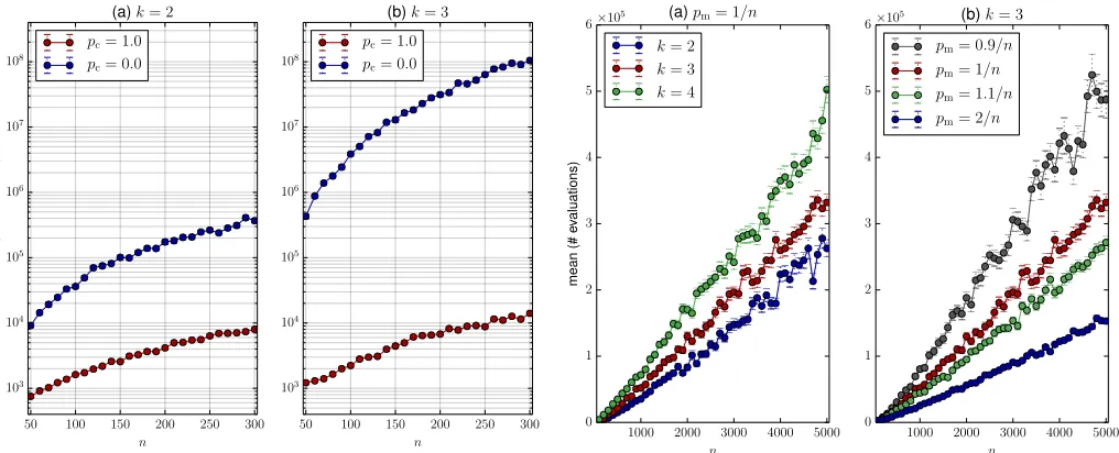
Figure 3. The impact of enabling crossover.
4e lnnso that a realistic population of at least40individuals is always assumed (e. g., even for n= 50in Figure 3).
A. Impact of crossover and mutation rates
Figure 3 (a) and (b) depict the performance of the GA (pc=
1.0) compared to the algorithm using only mutation (pc= 0.0)
under the same setting (pm = 1/n). The range of n in this
experiment is set to n= [50. . .300]with a step size of 10, andkis in{2,3}. Even with these small values ofkandn, a strong reduction of the average run time can be observed, up to a multiplicative factor of104.
The impact of the jump lengthkon the run time is illustrated in Figure 4 (a). The experiment was set withnin[100. . .5000] (with a step size of 100) and k is in {3,4,5}. We notice that the increase of k does not imply a large change in the average run time. The average run time seems to still scale linearly with n in this setting even for k = 4. By fixing
k = 3, we also experimented with different mutation rates, i.e.,pmin{0.9/n,1/n,1.1/n,2/n}. The results are displayed
in Figure 4 (b). We notice that the mutation rates above 1/n
reduce the average run time while a slightly lower mutation rate increases it considerably. With mutation rate 2/n, the average run time and the stability of the runs are distinctively improved.
On the other hand, an excessive increase of the mutation rate may deteriorate the average run time because of the likelihood of multiple bit flips which imply harmful mutations. This can be observed in the experiment depicted in Figure 5 (in log-scale) forn= 500. In this experiment,kis in{2,3,4}, and the range ofχ=pm·nis set to[0.6. . .8](with a step size of0.1).
We note that the morekis increased, the stronger the negative effect of high mutation rates can be noticed. Moreover, too low mutation rates are also bad for the run time. This can be related to our theoretical analysis, in which a low mutation rate could have made the random walk associated with the size of the largest species biased toward the wrong direction. This may
1000 2000 3000 4000 5000
n
0 1 2 3 4 5 6
mean
(#
ev
aluations)
×105 (a)pm= 1/n
k= 2
k= 3
k= 4
1000 2000 3000 4000 5000
n
0 1 2 3 4 5
6×10⁵ (b)k= 3
pm= 0.9/n
pm= 1/n
pm= 1.1/n
pm= 2/n
Figure 4. Run time for different jump lengthskand different mutation rates pmwith crossover.
lead to the reduction of the population diversity and the loss of benefit from crossover.
B. Comparison with the use of diversity mechanisms
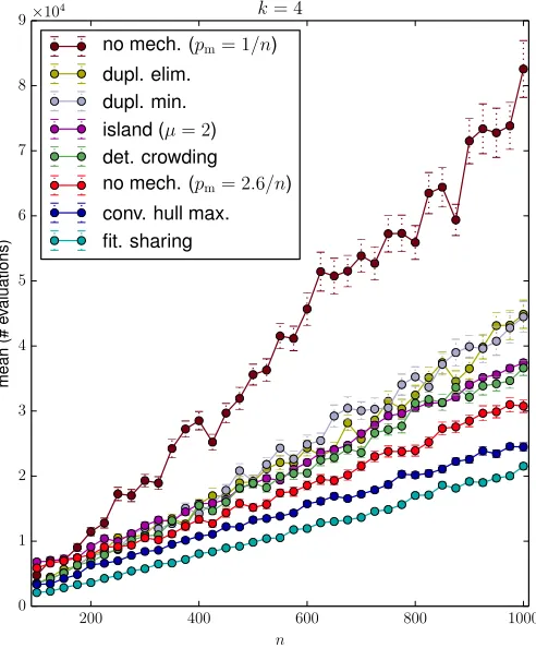
In a previous study [7], we have shown that many common mechanisms to preserve population diversity can speed up significantly the expected optimisation time of (µ+1) GA (with standard mutation rate) onJumpk when crossover is enabled. The aim of this section is to compare by experiments the setting of high mutation rate with the results taken directly from [7] for six1 mechanisms: duplicate minimisation and elimination, deterministic crowding, convex hull maximisa-tion, fitness sharing and island model.
Again full crossover is enabled (pc= 1.0), but the problem
size n is varied in [100,1000] (with a step size of 25). The result fork= 4is shown in Figure 6 which also includes the setting of (µ+1) GA with standard mutation rate and without any diversity mechanism as a reference. Here the high muta-tion rate is set withpm= 2.6/n (the best choice forn= 500
andk= 4, previously suggested by Figure 5). An interesting observation from the experimental results is that it appears the setting of high mutation rate can be as efficient as the implementation of specific diversity mechanisms. Specifically, in Figure 6 the setting of high mutation rate is only worse than convex hull maximisation and fitness sharing.
VIII. CONCLUSION
A rigorous analysis of the (µ+1) GA has been presented showing how combining the use of crossover with that of mutation considerably speeds up the run time for Jumpk compared to algorithms using mutation only.
It is traditionally believed that crossover is useful only in the presence of sufficient diversity, and the emergence of this
diversity is typically attributed to the mutation operator [11], [15], [35]. In general, the dynamics of mutation and crossover are vastly complex, and the question of how the two operators interact to balance exploration and exploitation has been open for decades [30]. Nevertheless, previous theoretical results on the benefit of crossover have relied solely on mutation for establishing the diversity necessary for recombination. For example, on the Jumpk function (with the exception of our own work in [7]), proofs have required an unrealistically small crossover probability in order to force long phases during which mutation alone builds up enough diversity before a useful crossover operation can be applied.
Diversity can also be enforced using artificial mechanisms, and such techniques lead to more efficient evolutionary algo-rithms both empirically [4], [32] and theoretically [13], [28]. Artificially enforced diversity can also be used in proofs that crossover is beneficial without having to rely on mutation alone to create sufficient variation [7].
The question to what degree the interplay between both crossover and mutation promotes the natural emergence of diversity in the population has been so far open. Our analysis shows that this interplay on the plateau of local optima of the Jumpk function quickly leads to a burst of diversity that is then exploited by both operators to reach the global optimum. The balance between the amount of mutation and crossover impacts the run time considerably. While mutation rates lower than the standard 1/n rate considerably increase the expected run time, rates that are slightly higher than 1/n lead to im-proved performance. These rates also depend on the presence of crossover. For instance, for k = 4, the best rate for a mutation-only algorithm is 4/n while the best rate for the (µ+1) GA with pc = 1 is considerably lower than 4/n and
higher than 1/n.
It is an open problem for future work whether crossover can lead to more than linear speedups onJumpk for realistic crossover probabilities. Our analysis could be improved by taking into account crossover between plateau individuals with Hamming distance larger than 2. For large k, this could lead to super-linear speedups. In fact, our experiments reveal that the average run time of the (µ+1) GA does not increase considerably when k is increased from 2 to 4. However, completely new techniques may be required to improve our analysis. Finally, future work should address the interplay between mutation and crossover on fitness landscapes with different characteristics than the Jumpk function, such as those featuring neutral networks.
Acknowledgements
The research leading to these results has received funding from the European Union Seventh Framework Programme (FP7/2007-2013) under grant agreement no. 618091 (SAGE) and from the EPSRC under grant no. EP/M004252/1. This research benefitted from Dagstuhl seminar 16011 ‘Evolution and Computing’ and is based upon work from COST Action CA15140 ‘Improving Applicability of Nature-Inspired Optimi-sation by Joining Theory and Practice (ImAppNIO)’ supported by COST (European Cooperation in Science and Technology).
1 2 3 4 5 6 7 8
χ
104 105 106
mean
(#
ev
aluations)
n= 500
[image:12.612.314.563.56.256.2]k= 2 k= 3 k= 4
Figure 5. The impact of different mutation ratespm=χ/nwith crossover
for a problem size of500.
200 400 600 800 1000
n
0 1 2 3 4 5 6 7 8 9
mean
(#
ev
aluations)
×104 k= 4
no mech. (pm= 1/n)
dupl. elim. dupl. min.
island (µ= 2)
det. crowding
no mech. (pm= 2.6/n)
conv. hull max. fit. sharing
Figure 6. The performance of the diversity mechanisms for jump length4; the mutation ratepmis set to1/nunless specified.
REFERENCES
[1] A. Auger and B. Doerr,Theory of Randomized Search Heuristics. World Scientific, 2011.
[image:12.612.315.561.301.598.2][3] N. Barton and T. Paix˜ao, ‘Can quantitative and popula-tion genetics help us understand evolupopula-tionary computa-tion?’, in Proc. of GECCO ’13, 2013, pp. 1573–1580. [4] N. Chaiyaratana, T. Piroonratana and N. Sangkawelert,
‘Effects of diversity control in single-objective and multi-objective genetic algorithms’, J. Heuristics, vol. 13, pp. 1–34, 2007.
[5] D. Corus, D.-C. Dang, A. V. Eremeev and P. K. Lehre, ‘Level-based analysis of genetic algorithms and other search processes’, in Proc. of PPSN XIII, 2014. [6] D.-C. Dang, T. Friedrich, T. Kotzing, M. Krejca, P. K.
Lehre, P. Oliveto, D. Sudholt and A. Sutton, ‘Emergence of diversity and its benefits for crossover in genetic algorithms’, inProc. of PPSN XIV, 2016, pp. 890–900. [7] ——, ‘Escaping local optima with diversity mechanisms and crossover’, inProc. of GECCO ’16, 2016, pp. 645– 652.
[8] B. Doerr, C. Doerr and F. Ebel, ‘From black-box complexity to designing new genetic algorithms’,Theor. Comput. Sci., vol. 567, pp. 87–104, 2015.
[9] B. Doerr, E. Happ and C. Klein, ‘Crossover can prov-ably be useful in evolutionary computation’, Theor. Comput. Sci., vol. 425, pp. 17–33, 2012.
[10] S. Droste, T. Jansen and I. Wegener, ‘On the analysis of the (1 + 1) Evolutionary Algorithm’,Theor. Comput. Sci., vol. 276, pp. 51–81, 2002.
[11] L. J. Eshelman, ‘Genetic algorithms’, in Handbook of Evolutionary Computation, Oxford University Press, 1997.
[12] W. Feller,An Introduction to Probability Theory and Its Applications. John Wiley & Sons, 1968.
[13] T. Friedrich, P. S. Oliveto, D. Sudholt and C. Witt, ‘Analysis of diversity-preserving mechanisms for global exploration’,Evol. Comput., vol. 17, pp. 455–476, 2009. [14] B. W. Goldman and W. F. Punch, ‘Fast and efficient black box optimization using the parameter-less popu-lation pyramid’, Evol. Comput., vol. 23, pp. 451–479, 2015.
[15] Handbook of Genetic Algorithms. Van Nostrand Rein-hold, 1991.
[16] J. He and X. Yao, ‘A study of drift analysis for estimat-ing computation time of evolutionary algorithms’, Nat. Comput., vol. 3, pp. 21–35, 2004.
[17] T. Jansen, Analyzing Evolutionary Algorithms – The Computer Science Perspective. Springer, 2013. [18] T. Jansen and I. Wegener, ‘The analysis of evolutionary
algorithms – a proof that crossover really can help’,
Algorithmica, vol. 34, pp. 47–66, 2002.
[19] N. L. Komarova, E. Urwin and D. Wodarz, ‘Accelerated crossing of fitness valleys through division of labor and cheating in asexual populations’,Scientific Reports, 2012.
[20] T. K¨otzing, D. Sudholt and M. Theile, ‘How crossover helps in pseudo-boolean optimization’, in Proc. of GECCO ’11, 2011, pp. 989–996.
[21] P. K. Lehre and X. Yao, ‘Crossover can be constructive when computing unique input–output sequences’, Soft Comput., vol. 15, pp. 1675–1687, 2011.
[22] K.-F. Man, K.-S. Tang and S. Kwong, ‘Genetic algo-rithms: concepts and applications’, IEEE Trans. Ind. Electron., vol. 43, pp. 519–534, 1996.
[23] F. Neumann, P. S. Oliveto, G. Rudolph and D. Sudholt, ‘On the effectiveness of crossover for migration in par-allel evolutionary algorithms’, inProc. of GECCO ’11, 2011, pp. 1587–1594.
[24] F. Neumann and C. Witt, Bioinspired Computation in Combinatorial Optimization – Algorithms and Their Computational Complexity. Springer, 2010.
[25] P. S. Oliveto, J. He and X. Yao, ‘Analysis of population-based evolutionary algorithms for the vertex cover prob-lem’, inProc. of CEC ’08, 2008.
[26] P. S. Oliveto and C. Witt, ‘On the runtime analysis of the simple genetic algorithm’,Theor. Comput. Sci., vol. 545, pp. 2–19, 2014.
[27] ——, ‘Improved time complexity analysis of the sim-ple genetic algorithm’, Theor. Comput. Sci., vol. 605, pp. 21–41, 2015.
[28] P. S. Oliveto and C. Zarges, ‘Analysis of diversity mechanisms for optimisation in dynamic environments with low frequencies of change’,Theor. Comput. Sci., vol. 561, pp. 37–56, 2015.
[29] A. Pr¨ugel-Bennett, ‘Benefits of a population: five mech-anisms that advantage population-based algorithms’,
IEEE Trans. Evol. Comput., vol. 14, pp. 500–517, 2010. [30] W. M. Spears, ‘Crossover or mutation?’, in Proc. of
FOGA II, 1992, pp. 221–237.
[31] D. Sudholt, ‘Crossover speeds up building-block assem-bly’, inProc. of GECCO ’12, 2012, pp. 689–696. [32] R. K. Ursem, ‘Diversity-guided evolutionary
algo-rithms’, inProc. of PPSN VII, 2002, pp. 462–474. [33] D. B. Weissman, M. W. Feldman and D. S. Fisher, ‘The
rate of fitness-valley crossing in sexual populations’,
Genetics, vol. 186, pp. 1389–1410, 2010.
[34] C. Witt, ‘Runtime analysis of the (µ + 1) EA on simple pseudo-Boolean functions’,Evol. Comput., vol. 14, pp. 65–86, 2006.
[35] M. ˇCrepinˇsek, S.-H. Liu and M. Mernik, ‘Exploration and exploitation in evolutionary algorithms: a survey’,