A Semiparametric Bayesian Approach to a New Dynamic Zero-Inflated Model

A Semiparametric Bayesian Approach to a New Dynamic

Zero-Inflated Model

Kiranmoy Das, Bhuvanesh Pareek, Sarah Brown, and Pulak Ghosh

ISSN 1749-8368

SERPS no. 2017001

A Semiparametric Bayesian Approach to a New

Dynamic Zero-Inflated Model

Kiranmoy Das, Bhuvanesh Pareek, Sarah Brown*, and Pulak Ghosh

January 14, 2017

Abstract

We develop a dynamic zero-inflated model to analyse the number of hospital ad-missions within an aging population, which allows for the considerable number of zero

hospital admissions at the individual level and occurrence dependence. In addition, certain health conditions may lead to groups of individuals having similar hospital

ad-mission rates. We analyse the US Health and Retirement Survey, which includes self-assessed health (SAH), which can be predictive of hospital admissions. Our modelling framework embeds a dynamic hierarchical matrix stick-breaking process to flexibly

characterize this dynamic group structure allowing individuals to belong to different SAH groups at different points in time.

Key Words: Bayesian models; Dirichlet process; Dynamic hurdle; Lasso; Matrix stick-breaking process; Zero-inflated data.

JEL Classifications: C11; C14; I12

Kiranmoy Das is Assistant Professor, Indian Statistical Institute, Kolkata, India; Bhuvanesh Pareek is Assistant Professor, Indian Institute of Management, Indore, India; Sarah Brown is Professor of Economics at University of Sheffield, UK; Pulak Ghosh is Professor, Department of Decision Sciences and Information Systems, Indian Institute of Management, Bangalore, India.

1

Introduction

The fact that the world population is aging is well-established: as stated by the United Nations (2015), ‘virtually every country in the world is experiencing growth in the number and proportion of older persons in their population.’ Specifically, their latest estimates predict that between 2015 and 2030, the number of people in the world aged 60 years or over is projected to grow by 56 per cent, from 901 million to 1.4 billion. With respect to increases in life expectancy, the World Health Organisation (2016) reports US life expectancy at 79.3 years in 2015, compared to 66.6 years in 1960 and 46.3 years in 1900. It is apparent that such demographic changes will be associated with an increased demand for health care, as well as, changes in the nature of health care demand, with needs associated with chronic conditions becoming increasingly important. It is crucial, therefore, that we enhance our understanding of the demand for health care.

Hospital admissions are an important aspect of the demand for health care and, further-more, it is apparent that as chronic conditions become more prevalent in the context of an aging population, understanding the needs associated with inpatient care and hospital visits becomes increasingly important. As aging changes the nature of health care demand with more emphasis on hospitalization and thus more challenges faced by health care systems throughout the world, further analysis into hospital admissions at the individual level seems to be particularly warranted. Thus, in this paper, we contribute to the existing literature which has focused on developing models to analyse the rate of hospital admissions at the individual level. We exploit data drawn from the US Health and Retirement Survey, which provides detailed information following individuals over time for an aging population. A number of analytical challenges associated with modelling hospital admissions at the in-dividual level have been discussed in the existing literature, which serves to highlight the complexities associated with modelling the demand for health care. Such challenges have generally not been addressed within a unified framework. Thus, we aim to fill this gap in the existing literature by conducting a comprehensive study of these issues. We now discuss these analytical challenges in more detail.

analyse the number of hospital admissions at the individual level in the context of an aging population. Simple distributions such as the Poisson or log normal distributions have been used to model count variables such as the number of hospital admissions. However, such an approach does not allow for the ordering information, which is likely to be inherent in such data: i.e., an individual who was hospitalised 3 times may be regarded as more serious compared to an individual who was hospitalised once in the same year. Hence, in this paper, we propose an ordered logistic regression approach, i.e. a proportional odds model, to analyse the number of hospital visits. Furthermore, as expected, there are a considerable proportion of zero observations in our data, on average, 84%, which is based on the US Health and Retirement Survey (HRS), reflecting the fact that a significant proportion of individuals are not admitted to hospital in a given year. In order to account for such inflation at zero, we develop an approach based on a zero-inflated proportional odds model.

Finally, categories of self-assessed-health (SAH), where respondents rate their own general health on a response scale from say poor to excellent, have been used extensively in the health economics literature. SAH is regarded as a good proxy for health risk since it contains private information on health and health related behaviours that are predictive of future health and are known only to the respondent. Idler and Benyamini (1997), for example, show that SAH is predictive of mortality even after conditioning on objective measures of health. It is often useful to group individuals based on covariate characteristics and in our application it is interesting to group individuals according to their SAH. Furthermore, in the HRS data, these groups can be dynamic with SAH varying over time. Within a time-varying group structure, stronger dependence is expected among the data temporally close to each other. Thus, it is interesting to develop models where one can estimate the group-specific parameters by efficiently borrowing information across the groups dynamically in an automated manner.

Dirichlet Process (DP) priors have been successfully used in a wide range of applica-tions for borrowing information across groups in an automated manner. Some examples include Ferguson (1973), Antoniak (1974), Blei and Jordan (2006), Dunson, Herring, and Engel (2008) and Rodriguez and Dunson (2014). Dunson et al. (2008) developed a matrix stick-breaking process (MSBP) which is an important extension of the usual DP. MSBP is essentially a generalization of the stick-breaking structure of DP (Sethuraman, 1994) where the row and column stick-breaking random variables induce dependent local clustering. In this paper, we first extend the stick-breaking weights into a product of group, time and predictor specific components and then induce extra dependence among the data that are temporally close to each other following Ren et al. (2010). The resultant proposed dynamic hierarchical MSBP (DH-MSBP) is powerful because here we allow: (i) multiple shrinkage of a large set of model parameters; (ii) global and local clustering by borrowing information within and across groups; and (iii) a higher probability of sharing the same set of parameters for temporally close data points.

2

A Zero-Inflated Dynamic Hurdle Proportional Odds

Model

Here we consider modelling hospital visits as our dependent variable. We distinguish between two types of individual: (i) those who started visiting hospitals from the very first wave (the start of the survey) until the end, and (ii) those who did not visit hospital initially but then started visiting after a few waves.

Define Yirt as the count of hospital visits for thei-th individual in the r-th health status

(self-assessed) group at wave t (t = 1,2, . . . ,10). Health status is based on self-assessment and can be categorized as “poor”, “fair”, “good”, “very good”, “excellent”. These health states can obviously vary over time. Thus, we have a very general set-up.

Our base model is the following zero-inflated dynamic model for Yirt:

Yirt= (1−πirt)1[Yirt=0]+πirtG(Yirt|Yirt>0), (1)

where, πirt is the probability of hospital admission, i.e., πirt=P(Yirt >0), and G(Yirt|Yirt>

0) is the distribution of the count of hospital visits conditional on hospitalization. In general,

when an individual visits hospital in a year, Yirt can take any of the values among k =

1,2,· · · , K.

2.1

Model for

π

For modelling the proportion of non-zeros, we consider a Probit model and thus expressπirt

as the following: Φ−1_(π

irt) =xTi δ+ηi, where Φ denotes the cdf of the standard normal, and

xis the set of covariates (both with time-varying and time-invariant effects on the response)

andδis the vector of regression coefficients. The individual-specific random effectsηicapture

2.2

Modelling

G

(

Y

|

Y

>

0)

The distribution of the count of hospital visits, i.e., G(Yirt|Yirt>0) can be of two types: (1)

individuals who visit the hospital for the first time at the t-th wave and; (2) individuals who

visited the hospital before the t-th wave. We argue that the rate of hospitalization should

be different for these two types of individual who are exposed to hospital for the first time

att and who were exposed before t, respectively. We use a proportional odds model with a

dynamic hurdle component for case 1 following Baetschmann and Winkelmann (2016) and use a simple proportional odds model for case 2.

Case 1

Let t be the wave where the i-th individual visits hospital for the first time. In this case,

we follow Baetschmann and Winkelmann (2016) and use a dynamic hurdle Poisson model

for modelling G. This is based on the assumption that in this particular wave, for each

individual, the time of the first hospital visit and the total number of hospital visits are related to each other. Suppose the first hospital visit for individual i occurs at time, Ti; for

0< Ti < t. Therefore, one can write,

P r(Yirt=k, Ti) =P r(Yirt=k|Ti)f1(Ti) =P r(Yirt(Ti, t−Ti) =k−1)f1(Ti);

where Yirt(Ti, t−Ti) denotes the number of hospital visits for the i-th individual in thet-th

wave within the time interval (Ti, t−Ti), and f1 denotes the pdf of the time to the first hospital visit. The marginal distribution of Yirt, thus, can be obtained as:

P r(Yirt=k) =

Z t

t−1

P r(Yirt(Ti, t−Ti) =k−1)f1(Ti)dTi. (2)

We considerTi as the time to elapse before the event of interest (hospital admission) and

thus model this waiting time by a Weibull distribution. Specifically, we consider f1 as the

density of a Weibull distribution with parameters η1 and η2. Thus, Ti ∼Weibull(η1, η2).

The cdf of Yirt(Ti, t−Ti) is modelled by the following proportional odds model:

logit(P r(Yirt ≤k)) = J

X

j=1

αjkr(t)xij(t) + J0 X

j0₌₁

βj0_krz_ij0_t+b_i, (3)

for k = 1,2, . . . , K. We consider J time-varying covariates; the effect of the j-th covariate on the log odds at time tisαjkr(t), which is also considered to be time-varying. We consider

bi, capture the correlation among the measurements from the same individual at different

waves.

For modelling the dependence among the zero-response probabilities and non-zero re-sponse probabilities, we assume that (ηi, bi) jointly follow a bivariate normal density with

mean vector=0 and var(ηi) =ση2, var(bi) =σb2, correlation(ηi, bi) =ρ.

To model the time-varying coefficient αjkr(t) for the j-th covariate, we use penalized

splines (Ruppert, Wand and Carroll, 2003) and model αjkr(t) as follows:

αjkr(t) =bjkr0t+bjkr1tt+bjkr2tt2+...+bjkrgttgj+ Sj

X

s=1

cjkrst(t− Ts) gj

+, (4)

where (x)g+ =xgI(x >0) and (T1 <T2 < ... <TSj) is a fixed set of knots.

Case 2

Here the t-th wave indicates the waves after the i-th individual visited hospital for the first

time. For such waves, we model G as the proportional odds model. The cdf of Yirt(T) is

modelled by the proportional odds model given in equation (3).

3

A Nonparametric Bayesian Model for the time-varying

Coefficients

3.1

Dynamic Hierarchical Matrix Stick-Breaking Priors

time. The MSBP of Dunson et al. (2008) has practical advantages, in that individuals can be very similar for most of their coefficients, while still allowing distinct local deviations. Here we consider a novel extension of the MSBP where information is shared across the

self-reported health status groups (r) over the waves (t) for different numbers of hospital

admission (k).

Define the vector of polynomial coefficients from equation (4),bjkrt = [bjkr0t, bjkr1t, . . . , bjkrgjt]T.

Here we assume the vector bjkrt is drawn from an unknown distributionG(

b)

krt, which itself is

random, and a Dirichlet process (DP) is placed on the distribution ofG(_krtb).Thus, we assume,

bjkrt∼G( b)

krt= Nb

X

h=1

π(_krthb) δ_ξ(b)

th;

j = 1,2, . . . , J; k = 1,2, . . . , K; r = 1,2, . . . , R; t = 1,2, . . . , T,

ξ_th(b)∼G(_tb), (5)

whereδx denotes a point mass atx. Define Ξb =

ξ_th(b)to be a matrix of orderT×Nb, the

rows of which correspond to the parameters with the base distributionG(_tb) and the columns

correspond to the “clusters”. The stick-breaking weights π_krth(b) are defined as the following:

π_krth(b) =V_krth(b) Y

s0_<h

(1−V_krts(b)0); V (b)

krth =U

(b)

khZ

(b)

rhW

(b)

th ,

U_kh(b) iid∼Beta(1, δ₁(b)); Z_rh(b) iid∼Beta(1, δ₂(b)); W_th(b) iid∼Beta(1, δ₃(b)). (6)

The stick-breaking weights π_krth(b) control the dependence among the distributions G(_krtb). Note that we partition π_krth(b) into three components U_kh(b), Z_rh(b) and W_th(b) which allocate the

vector of the polynomial coefficients from thek number of hospital visits and ther-th health

status group and the t-th wave to theh-th cluster. We need to take V_krtN(b)

b = 1, for all k, r, t;

to make G(_krtb) a valid probability measure.

The dynamic nature of our setting requires stronger dependence among the distributions of parameters close to each other temporally. We propose the following hierarchical dynamic DP (Ren et al., 2010) for G(tb):

G(_tb) = (1−ω_t(₋b)₁)G_t(b₋)₁+ω_t(₋b)₁H_t(₋b)₁,

ωt(b)|αω, βω ∼Beta(αω, βω); αω ∼Gamma(ν1, ν2); βω ∼Gamma(κ1, κ2),

G₁(b) ∼DP(α₀₁(b), G(₀b)); H_t(₋b)₁ ∼DP(α₀(b_t), G(₀b)),

In the above prior, we note that G(tb) is identical to G

(b)

t−1 with probability 1−ω (b)

t−1 and with probabilityωt(−b)1 it is identical to an innovation distribution, H

(b)

t−1. A Dirichlet Process Prior (DPP) is considered for the innovation distribution. For the base distribution G(₀b) we further consider a DPP similar to the hierarchical Dirichlet process (HDP) proposed by Teh et al. (2006). The key point to note is that the above prior not only encourages “information exchange” among the temporally proximate parameters but also for the temporally distant parameters.

Formulations 5, 6 and 7 complete our proposed structure for the dynamic MSBP.

For the set of spline coefficients cjkrt = [cjkr1t, cjkr2t, . . . , cjkrSjt]T in (4), we similarly

specify the following dynamic MSBP prior:

cjkrt ∼G

(c)

krt; j = 1,2, . . . , J; k = 1,2, . . . , K; t= 1,2, . . . , T,

G(_krtc) =

Nc

X

h=1

π_krth(c) δ_ξ(c)

th;

π(_krthc) =V_krth(c) Y

s0_<h

(1−V_krts(c)0); V (c)

krth=U

(c)

khZ

(c)

rhW

(c)

th ,

U_kh(c) iid∼Beta(1, δ₁(c)); Z_rh(c)iid∼Beta(1, δ(₂c)) W_th(c)iid∼Beta(1, δ₃(c)),

ξ_th(c) ∼G(tc); G

(c)

t = (1−ω

(c)

t−1)G (c)

t−1+ω (c)

t−1H (c)

t−1,

G₁(c)∼DP(α₀₁(c), G₀(c)); Ht(−c)1 ∼DP(α (c) 0t, G

(c) 0 ),

G₀(c)∼DP(γ₀(c), H(c)); H(c) ∼N(µ0, λ−1I); λ∼Gamma(α∗, β∗). (8)

We note that the above prior is very similar to the priors proposed in (5-7) except the

prior for H(c). The spline coefficients essentially measure the roughness at the respective

knots and one can make the function smoother by shrinking the roughness towards zero. In a Bayesian framework, this is achieved by considering a multivariate normal prior with the

covariance matrix λ−1I for the base distribution H(c) _{and then placing a gamma prior on}

the penalty parameter λ, (Das and Daniels, 2014).

3.2

Properties

Note that the features of our proposed DH-MSBP priors forbjkrt and cjkrt, for j = 1, . . . , J,

have the same form. Here we focus on the properties of the prior for bjkrt only. Details of

the other properties of the MSBP and dynamic DP can be found in Dunson et al. (2008) and Ren et al. (2010).

We note that the dynamic structure of G(tb) can be expressed as: G

(b)

t = (1−ω

(b)

t−1)G (b)

ω_t(₋b)₁H_t(₋b)₁ = ˜ω(_t1b)G₁(b) + ˜ω_t(₂b)H₁(b) +. . .+ ˜ωtt(b)H

(b)

t−1, where ˜ω (b)

tl = ω

(b)

l−1

t−1 Q

m=1

(1−ωm(b)), for l =

1,2, . . . , t.

Proposition 1

Consider sets A in the Borel field of the real line. AsNb → ∞, we have

E{G(_krtb)(A)}=

t

P

l=1 ˜

ω(_tlb)H(b)_(A),

V{G(_krtb)(A)}=

t

P

l=1 ˜

ω(_tlb)2

1+α(₀b_l)

α(₀b_l)+γ₀(b)+1 1+γ₀(b)

H(b)(A){1−H(b)(A)}

1− 4

(δ(₁b)+2)(δ₂(b)+2)(δ(₃b)+2)−4

+ 4

(δ(₁b)+2)(δ₂(b)+2)(δ(₃b)+2)−4

t

P

l=1 ˜

ω_tl(b)H(b)_(A) 1− t P l=1 ˜

ω_tl(b)H(b)_(A)

.

Proof: As Nb → ∞ we have,

E{G(_krtb)(A)}=EE{G_krt(b)(A)|G(tb)}=E{

∞

P

h=1

π(_krthb) δ_ξ(b)

th

(A)|G(tb)}

=E{G(_tb)(A)}= ˜ω_t(₁b)H(b)_{(A) + ˜ω}(b)

t2 H(b)(A) +. . .+ ˜ω (b)

tt H(b)(A) = t

P

l=1 ˜

ω(_tlb)H(b)_(A).

From Dunson et al. (2008), it follows that

V{G(_krtb)(A)}=

1− 4

(δ(₁b)+2)(δ(₂b)+2)(δ₃(b)+2)−4 V{G (b)

t (A)}+

E{G(tb)(A)}

2

+ 4

(δ(₁b)+2)(δ₂(b)+2)(δ(₃b)+2)−4E{G (b)

t (A)} −

h

E{G(tb)(A)}

i2

.

Since G(tb) has a dynamic structure, from Ren et al. (2010), we have,

V{G(tb)}= t

P

l=1 ˜

ω(_tlb)2

1+α(₀b_l)

α(₀b_l)+γ₀(b)+1 1+γ₀(b)

H(b)_(A){1−H(b)_{(A)}. We also use the fact thatE{G}(b)

t (A)}= t

P

l=1 ˜

ω_tl(b)H(b)_{(A). The expression for V{G}(b)

krt(A)} then follows immediately.

Proposition 2

For the proposed DH-MSBP prior:

(a) the probability that for fixed timet, and fixed value k, the health status groups r andr0

will have identical coefficients for the polynomial part of (4) is

P r(bjkrt=bjkr0t) = 2

(b) the probability that the health status group r will have identical coefficients for the polynomial part of (4) at two different times t and t0_{, for a fixed value k is:}

P r(bjkrt=bjkrt0) = 2

(δ(₃b)+1)(δ₁(b)+2)(δ(₂b)+2)−2;

(c) the probability that the health status groupr will have identical coefficients at fixed time

t for the polynomial part of (4) at two different values k and k0 is

P r(bjkrt=bjk0_rt) = 2

(δ(₁b)+1)(δ₂(b)+2)(δ(₃b)+2)−2.

The proofs of the above results are similar to Dunson et al. (2008), and hence are omitted here for brevity.

Note that the prior clustering probabilities in (a), (b), and (c) range between 0 and 1 depending onδ₁(b),δ₂(b) andδ(₃b). Clearly ifδ₁(b), δ₂(b), δ₃(b) →0, then the clusters are not different and all the above prior probabilities converge to 1. However, for δ₁(b) or δ₂(b) or δ(₂b) → ∞, none of the sets are clustered together and thus the probabilities in (a), (b) and (c) converge to 0.

3.3

Zero-Inflated LASSO Priors

Since we have a large number of covariates with time-invariant effects on our response vari-able, we incorporate a shrinkage prior approach. Our approach is similar to the hierarchical Bayes representation of the LASSO proposed by Park and Casella (2008). Recently, Das (2016) proposed a modified Bayesian LASSO with a zero-inflated structure which is relevant to our setting. Define βkr = (β1kr,· · · , βJ0kr)T. We add sparsity to the prior and consider

the following hierarchical representation:

βj0_kr|σ2, τ_j20, Bj0 ∼(1−B_j0)δ₀+B_j0N 0, σ2τ_j20

,∀j0, k, r,

Bj0|π_j0 ∼Bernoulli(π_j0), π_j0 ∼Beta(u, v),

τj20 iid

∼ λ

2

2 exp

−1

2λτ 2

j0

, λ2 ∼π(λ2), σ2 ∼π σ2.

Here δ0 is a point mass probability measure at 0. Note that the parameters πj0s are

updated from the data and force the coefficients of the insignificant covariates to be exactly equal to 0 and simultaneously shrink the other coefficients towards 0 as LASSO does. The

advantage of considering a zero-inflated normal prior for βj0_kr is discussed in detail in Das

3.4

Joint Posterior and Computational Details

Note that the likelihood function of the longitudinal responsesYirtcan be written as follows:

L=



 Y

(i,r,t):Yirt=0

(1−πirt)



×



 Y

(i,r,t):Yirt>0

πirtG(Yirt|Yirt>0)

  (9) = Z Z     Y

(i,r,t):Yirt=0

(1−Φ(xT_i δ+ηi)



×



 Y

(i,r,t):Yirt>0

Φ(xT_i δ+ηi)G(Yirt|bi)



 

f(ηi, bi)dηidbi,

where G(Yirt|bi) is the density described in Section 2.2 and f(ηi, bi) is the joint density of

the random effects. The log likelihood function can be expressed accordingly. The joint

posterior distribution is obtained by multiplying the corresponding prior components to L.

Note that for δ (Section 2.1), we consider a multivariate normal prior with mean vector=0

and covariance matrix=σ_δ2I. Priors for all the other model parameters are discussed in

Sections 3.1 and 3.2.

We note that the truncation of the MSBP to finiteNb (and also forNc) is done using the

approximation in Ishwaran and James (2002), such that the truncation value (Nb) makes

the expected approximation error smaller than 0.01. For bjkrt, the expected approximation

error =

1− 1

(1+δ(₁b))(1+δ₂(b))(1+δ₃(b)) Nb−1

, which requires knowing δ₁(b), δ₂(b), and δ₃(b). Following

Dunson et al. (2008), we specify independent gamma(1,1) priors forδ₁(b),δ₂(b) andδ(₃b) and we run the MCMC algorithm for about 15% of its total length and use the posterior means of

δ₁(b), δ₂(b) and δ₃(b) to determine if the expected approximation error is below 0.01. The same

approach is used to choose Nc. Our computations are similar to Das and Daniels (2014),

Chatterjee et al. (2016).

4

Simulation Study

We investigate the operating characteristics of the dynamic hurdle model and the dynamic hierarchical MSBP prior through simulation studies. We consider a zero-inflated longitudinal count response, two covariates with time-varying effects and 10 covariates with time-invariant effects on the response.

We simulate data for 100 subjects at 10 evenly spaced time points (t = 1,2, . . . ,10).

Consider 4 groups (r = 1,2,3,4) and each subject belongs to one of these 4 groups at each

time point. In particular, we consider 30 subjects who are in group 1 until t = 6, and then

belong to group 2; 10 subjects who change from group 1 to group 4 at t = 5. Consider 20

subjects who change from group 2 to group 3 at t= 7; 10 subjects who change from group

2 to group 4 at t = 4; 10 subjects change from group 3 to group 1 at t = 5; 10 subjects

change from group 3 to group 4 at t = 6, and 10 subjects move from group 4 to group 1

at t = 8. We simulate the response Yirt from the model given in equation (1), where the

non-zero mixing proportions, πirts, are simulated from the probit model given in Section

2.2 (the explicit form of which is given in the web-appendix). If for the t-th time point we

observe the first non-zero response, then Yirt is generated from the model given in equation

(2) with Ti ∼W eibull(1,5) and the cdf of Yirt(Ti, t−Ti) is obtained from equation (3) with

k = 0, . . . ,5, J = 2 and J0 = 10. On the other hand, if the t-th time point is either the time

before or after the time of the first occurrence of the event, we then simulate Yirt from the

model given in equation (3). We consider the following spline function for αjkr(t):

αjkr(t) =bjkr0t+bjkr1tt+bjkr2tt2+

2 X

s=1

cjkrst(t− Ts)2+, (10)

with the knots T1 = 3 andT2 = 7. We consider both the discrete and continuous covariates

with time-invariant effects on the response. These covariates are simulated from Normal and Bernoulli distributions. The details of the parameter values for the simulation are given in the web-appendix. In general, we consider the different parameter values across the groups

and times for different k to be somewhat similar but not exactly the same.

non-dynamic hurdle, where G(Yirt|Yirt > 0) is modelled for all the subjects at all the time

points using the proportional odds model given in equation (3).

We simulate 100 datasets and for each dataset we run the MCMC algorithm for 65,000 iterations, discard the first 5,000 (“burn-in”) and thin the remaining 60,000 by keeping every 10-th iteration. The model parameters are estimated using posterior means. We specify

Nb =Nc = 20, which gives a truncation approximation error less than 0.015.

For the model selection, we use the conditional predictive ordinate (CPO) (Gelfand et al. 1992) defined as CP Oi = P(Yi|Y−i) = Eθ[P(Yi|θ, Y−i)], where Y−i denotes the data

excluding Yi and θ denotes the set of all model parameters. For the i-th subject, the CPO

can be estimated based on the MCMC samples as the following:

[

CP Oi =

1

M M

P

m=1 1

P(Yi|θ(m)₎ −1

, where θ(m) _{denotes the parameter estimates at the m-th}

iteration of MCMC. We compute the log pseudo-marginal likelihood (LPML)=

n

P

i=1

logCP O[i,

where a greater value of the LPML indicates a better fit.

We compute the LPML across all replications and Table 1 shows the average values for the different models. We note that the DH-MSBP prior with a dynamic hurdle gives the largest LPML value. However, the LPML values for the DH-MSBP prior with the non-dynamic hurdle and the group-specific model with the non-dynamic hurdle are quite close to this largest value.

5

Data Analysis

5.1

The HRS Data

We exploit data from the University of Michigan’s Health and Retirement Study (HRS), which is a longitudinal survey of Americans over the age of 50, with a follow-up frequency of every two years. The HRS provides multi-disciplinary data to understand the challenges of aging. In this paper, we use data for 10 waves from the 1931-1941 cohort. Baseline observations for this cohort began in 1992 when individuals were aged between 52 and 62, and, hence, were nearing retirement. The HRS is maintained by RAND’s Center for the Study of Aging. Our sampling is based on 2630 individuals, who are observed in all 10 waves. For our outcome measure, we use the number of hospital visits made since the previous interview. This variable is derived from the responses to the following question: How many different times were you a patient in a hospital overnight in the last 24 months? As expected, a large proportion of zero observations are observed in the data. Specifically, from waves 1 to 4, 90-94% are zero observations, which falls to 80-86% for waves 5 to 8, and to 75-80% for waves 9-10. In accordance with intuition, the proportion of zero observations declines as the individuals in our sample age. Across all waves, for the non-zero responses, the minimum value of the response variable is 1 and the maximum is 15, with an average of 1.4 visits. With respect to grouping individuals by health status, we have 5 categories of

SAH (r); poor (1), fair (2), good (3), very good (4) and excellent (5), which can vary over

time.

The HRS provides a rich set of covariates for our analysis. Specifically, we have four covariates with time-varying effects on the response variable, i.e. the number of hospital visits, namely: (i) the body mass index (BMI); (ii) the total value of assets, (iii) the total value of debt and (iv) total household income.

height. Hence, we include BMI in our modelling framework.

The inclusion of the three financial covariates reflects the large existing literature ex-ploring the relationship between a range of household financial outcomes and health. For example, Adams et al. (2003), Michaud and van Soest (2008) and Hurd and Kapteyn (2003) generally find a positive association between better health and household wealth. Total as-sets are defined as the summation of the value of: individual retirement accounts; stocks; bonds; checking and saving accounts; certificates of deposit and saving bonds; other saving accounts; the primary residence; transport; net value of any business; and other assets.

With respect to the other side of the household balance sheet, there is a growing literature exploring the relationship between health and debt. For example, Drentea and Lavrakas (2000) find that both credit card debt and stress regarding debt are inversely associated with good health and Brown et al. (2005) find that unsecured debt is inversely related to psychological wellbeing. More recently, Keese and Schmitz (2014) report that a variety of debt measures are strongly correlated with satisfaction with health and mental health. Our measure of total debt includes: all mortgages/land contracts; other home loans; and other debt including credit cards.

With respect to income, a number of studies have explored the relationship between income and health. For example, for the UK, Contoyannis and Rice (2001) report an inverse relationship which poor health and wages for men. For the US, Pelkowski and Berger (2004) use data from the US HRS and find that permanent health problems have a significant effect on labour market participation, wages and hours for both men and women. All monetary variables are entered in natural logarithm form and are expressed in 2010 prices.

different types of health insurance: (i) having health insurance related to employment; (ii) government insurance; and (iii) other private health insurance.

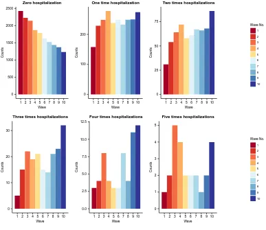
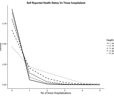
Some important features of the data are summarized in Figures 1 and 2 (as well as Figures S1 and S2 in the web appendix). In Figure 1, we show the counts of individuals with different numbers of hospital admissions across the 10 waves through a series of bar diagrams. We note that the counts decrease over the waves for zero admission and increase for the number of admissions 1, 2 and 3. For counts 4 and 5, there is no specific pattern evident although the counts are at the maximum for waves 9 and 10. In Figure 2, we show the distribution of individuals across the number of hospital admissions for each SAH category. We note that the distributions are neither the same nor completely different, but rather are similar in pattern for certain waves. This motivates the use of the dynamic MSBP construction as discussed earlier. In Figures S.1 and S.2 in the web appendix, we show the heat map of the average number of hospital admissions across the different SAH categories and waves; and total counts (from all SAH categories) across the number of hospital admissions for different waves.

5.2

Results

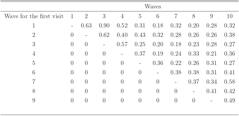
In Table 3, we show the distribution of the average number of hospital admissions for the individuals who made their first hospital visit at wave 1, 2, 3, etc. We observe clear differences in the distributions, reflecting the fact that the rates of hospital admission depend on the time of the first observed hospital visit. Under such a scenario, a dynamic hurdle model is more appropriate as demonstrated in Section 4.

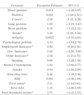
with the health covariates largely accord with our expectations. Health insurance related to employment and other private health insurance are both found to have significant effects, which may reflect better quality health care associated with such insurance relative to gov-ernment health insurance, leading to more frequent hospital visits for those holding such health insurance. Among the financial covariates, total assets and total household income exert significant effects on the probability of zero hospital visits. This is also not surprising since financially affluent individuals are more likely to be able to access health care thereby potentially leading to better health.

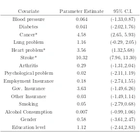
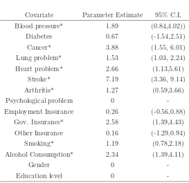
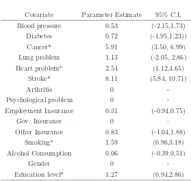
Next, in order to highlight the flexibility of our approach, we summarize the results for the covariates with time-invariant effects from equation (3) for different SAH categories and for

different values ofk. In Table 5, we present the corresponding coefficient estimates, and 95%

credible intervals (based on the MCMC samples) for the people belonging to the “good” SAH

group (r=3) with 1 or less hospital admissions. With respect to the chronic health conditions,

the findings as above accord with intuition, with the three particularly severe conditions, namely, cancer, heart problems and strokes, found to be statistically significantly related to the response variable, with large parameter estimates. The other controls are characterised by statistically insignificant parameter estimates. The large parameter estimates for educa-tion and government insurance are particularly noticeable. Educaeduca-tion is clearly related to employment opportunities as well as healthy life styles, (Cutler and Glaeser, 2005), whereas the large parameter estimate for government health insurance may reflect the importance of Medicare and Medicaid in the US. However, these parameter estimates are statistically insignificant in our case, since the 95% Credible intervals contain zero.

We then summarize the results for the two extreme SAH groups, i.e. the “poor” SAH group with the number of hospital admissions 4 or less; and the “excellent” SAH group

with 1 or less hospital admissions. Table 6 shows the results for the “poor” group with k

equalling 4 or less. Note that here we have some additional important covariates namely, blood pressure, lung problems, arthritis, smoking, alcohol consumption and government insurance. Coefficients for the covariates gender, education and psychological problems are exactly equal to 0, due to the zero-inflated LASSO prior. Table 7 summarizes the results for

the “excellent” SAH group withk=1. In addition to the chronic health conditions of cancer,

heart problems and stroke, smoking and education are found to be important predictors for this case.

covariates as mentioned earlier, namely: BMI, total assets, total debt and income. We have

5 categories of SAH (r); poor, fair, good, very good and excellent. Across all waves, SAH

is distributed as follows: excellent (21.66%); very good (38.78%); good (28.02%); moderate (9.00%); and poor (2.54%). In accordance with expectations, from waves 1 to 10, the proportion in the excellent SAH category falls as individuals age. For example, in wave 1, 32.40% are observed in the excellent SAH category, which falls to 21.53% by wave 5 and 12.85% by wave 10. For each of the four covariates with time varying effects on the number

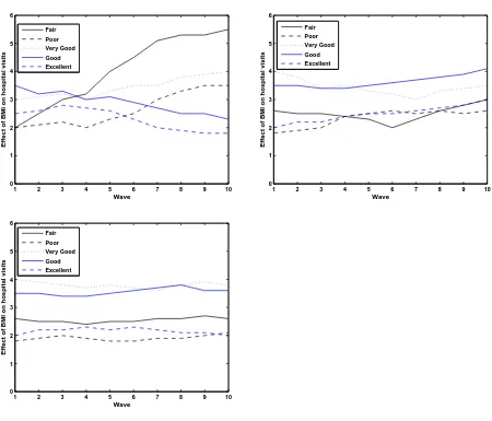
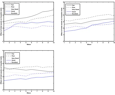
of hospital admissions, we present plots for these five categories of SAH for k=2, 4 and 6 for

illustration purposes.

Focusing initially on BMI, which is regarded as one of the leading indicators of health,

it is apparent from Figure 3 that, for k=2, the effect of BMI for the fair SAH category

increases dramatically over waves 1 to 10. In contrast, the effect of BMI for the poor category is characterised by a less pronounced increase from wave 4 onwards. Interestingly, the effects of BMI fall over the observed waves for the excellent and good SAH categories, yet demonstrate a steady increase over time for the very good health category. Furthermore,

the pattern of effects is clearly different for the case when k = 4, where less variation in the

pattern of the effects is apparent. For all 5 categories, we generally observe an increase in the effects over time, with the increase for the fair health category starting from wave 6 onwards

and for very good health, from wave 7 onwards. It is interesting to see that when k = 6, i.e.

for a very large number of hospital visits, distinct differences in the magnitudes of the effects are apparent across the five categories, with very good health generally characterised by the largest effect and poor health by the smallest. However, over the observed waves, the size of the effects within each SAH category are relatively stable, which clearly contrasts with the

case whenk = 2, where we observe considerable variation over time in the effects of BMI on

the outcome variable.

Turning to total financial assets, it is apparent that, when k=2 and k=4, for all five

SAH categories, in general, an upwards trend is observed moving from wave 1 to 10, with the size of the effects being most pronounced for the poor and fair SAH categories. The upwards trend is still apparent, yet less pronounced, for the other SAH categories. As in

the case of BMI, less variation in the effects of assets over the 10 waves is apparent when k

=2 relative to when k = 4, i.e. for a larger number of hospital visits. As expected, the poor

health category is characterised by the largest size of effect for k = 6. Focusing on excellent

SAH, it is apparent that across the values ofk, a moderate upwards trend can be seen across

effect of financial assets on the number of hospital visits within this SAH category being relatively stable over time. This contrasts, in particular, with the lower categories of SAH, specifically, poor and fair health, where the effect of financial assets appears to exhibit much

more variation over the waves, especially in the case where k = 2.

Interestingly in the case of debt, the observed patterns are generally the opposite to

those observed for financial assets. For example, when k = 2, a downwards trend is

gener-ally apparent for the effect of debt on hospital visits across the five SAH categories, with a particularly pronounced downwards trend apparent for the excellent and good SAH cate-gories. Thus, over waves 1 to 10, the findings suggest that the effect of debt on hospital visits

falls for k = 2, andk = 4. This may reflect the fact that over the life cycle debts generally

fall as individuals age: in an early seminal contribution, for example, Ando and Modigliani (1963) hypothesized that individuals may be more comfortable with debt holding when they are young and their income is low, as they expect future income to be much higher, and to be able to pay off the debt at a later stage. Thus, in the context of an aging population, the effect of debt on the number of hospital visits is generally seen to decline over time. Interestingly, in the case of the lowest two SAH categories, poor and fair SAH, a more stable effect is observed across all three cases, suggesting that the effect of debt does not fall for these categories. This may reflect borrowing associated with being in such low SAH states.

It is interesting to note that in the case where k = 6, all SAH categories, with the exception

of very good health, are characterised by an increase in the effect of debt on the number of hospital visits at wave 9.

Finally, with respect to income, the observed patterns tend to follow those associated with financial assets, with an upwards trend generally observed for all five SAH categories

across the three values of k. When k =2, the upwards trend is particularly pronounced

for the fair SAH category, with the very good health category characterised by the most

stable effect over time, which is also the case for the other values of k. It is interesting

to note that, although there are some changes in the relative size of the effect across the

three values of k, the effect of income on hospital visits seems to be relatively stable over

6

Discussion

In clinical trials and biomedical studies, dynamic group structure is not uncommon. For example, with respect to blood pressure an individual might belong to three different groups (high, medium and low) dynamically. Traditional approaches of analyzing clustered data do not work in such situations since the group sizes (and compositions) vary over time. Advanced nonparametric Bayesian methods allow information sharing across groups but the group structure is assumed to be static. We consider a dynamic group structure and develop models for handling the complexities with a zero-inflated longitudinal count measurement.

Our approach, however, suffers from one limitation. We assume no missingness in our data. However, in reality, it is not uncommon to have missing responses and some missing covariates. If the missingness is ignorable (e.g. missing at random), then one can simply add a data-augmentation technique to our method. However, for non-ignorable missingness our method has to be revised substantially following Daniels and Hogan (2008). Also one might have zero-inflated endogenous covariates with time-varying or time-invariant effects on the response. A Bayesian approach of two-stage regression could be developed for handling such cases. We leave these issues for future research.

References

1. Adams, P., Hurd, M. D., McFadden, D., Merrill, A., and T. Ribeiro, 2003, Healthy, wealthy, and wise? Tests for direct causal paths between health and socioeconomic status. Journal of Econometrics 112(1), 3–56.

2. Ando, A., and Modigliani, F, 1963, The“ life cycle” hypothesis of saving: Aggregate implications and tests. The American Economic Review 53(1), 55–84.

3. Antoniak, C.E, 1974, Mixtures of Dirichlet processes with applications to Bayesian non-parametric problems. The Annals of Statistics 2, 1152–1174.

5. Baetschmann, G. and Winkelman, R, 2016, A dynamic hurdle model for zero-inflated count data. Communications in Statistics-Theory and Methods (in press).

6. Banerjee, R., Ziegenfuss, J. Y., and Shah, N. D, 2010, Impact of discontinuity in health insurance on resource utilization. BMC Health Services Research 10(1), 1–10.

7. Brown, S., Taylor, K., and Price, S. W, 2005, Debt and distress: Evaluating the psycho-logical cost of credit. Journal of Economic Psychology 26(5), 642–663.

8. Blei, D. and Jordan, M, 2006, Variational inference for Dirichlet process mixtures. Bayesian Analysis 1, 121–144.

9. Chatterjee, A., Venkateswaran, P. and Das, K, 2016, Simultaneous state estimation for clustered based wireless sensor networks. IEEE Transactions on Wireless Communica-tions 15(12), 7985–7995

10. Contoyannis, P. and Rice, N, 2001, The impact of health on wages: Evidence from the British Household Panel Survey. Empirical Economics 26, 599–622.

11. Cutler, D. M. and Glaeser, E, 2005, What explains differences in smoking, drinking, and other health related behaviors? American Economic Review Papers and Proceedings 95(2), 238–242.

12. Das, K, 2016, A semiparametric Bayesian approach for joint modeling of longitudinal trait and event time. Journal of Applied Statistics 43(15), 2850–2865.

13. Das, K. and Daniels, M.J, 2014, A semiparametric approach to simultaneous covariance estimation for bivariate sparse longitudinal data. Biometrics 70, 33–43.

14. Deb, P. and Trivedi, P.K, 1997, Demand for medical care by the elderly: A finite mixture approach. Journal of Applied Econometrics 12, 313–336.

15. Drentea, P. and Lavrakas, P. J, 2000, Over the limit: the association among health, race and debt. Social Science and Medicine 50(4), 517-529.

16. Dunson, D., Herring, A. and Engel, S, 2008, Bayesian selection and clustering of poly-morphisms in functionally related genes. Journal of the American Statistical Association 103, 534–546.

Bayes meta-analysis. Journal of American Statistical Association 103(481), 317–327.

18. Ferguson, T.S, 1973, A Bayesian analysis of some nonparametric problems. The Annals of Statistics 1, 209–230.

19. Gelfand, A.E., Dey, D. and Chang, H, 1992, Model determination using predictive distri-butions with implementation via sampling based methods (with discussion). Bayesian Statistics 4, Eds: J. Bernardo et al. Oxford University Press, 147–167.

20. Hurd, M. and Kapteyn, A, 2003, Health, wealth, and the role of institutions. Journal of Human Resources 38(2), 386–415.

21. Idler, E. L. and Benyamini, Y, 1997, Self-rated health and mortality: a review of twenty-seven community studies. Journal of Health and Social Behaviour 38(1), 21–37.

22. Ishwaran, H. and James, L.F, 2002, Approximate Dirichlet process computing in finite normal mixtures. Journal of Computational and Graphical Statistics 11, 508-532.

23. Keese, M. and Schmitz, H, 2014, Broke, ill, and obese: Is there an effect of household debt on health? Review of Income and Wealth 60(3), 525–541.

24. Michaud, P. C. and Van Soest, A, 2008, Health and wealth of elderly couples: Causality tests using dynamic panel data models. Journal of Health Economics 27(5), 1312–1325.

25. Pelkowski, J. M. and Berger, M. C, 2004, The impact of health on employment, wages, and hours worked over the life cycle. Quarterly Review of Economics and Finance 44, 102–121.

26. Park, T. and Casella, G, 2008, The Bayesian Lasso. Journal of American Statistical Association 103, 681–686.

27. Ren, L., Dunson, D., Lindroth, S. and Carin, L, 2010, Dynamic nonparametric Bayesian models for analysis of music. Journal of the American Statistical Association 105, 458– 472.

28. Rodriguez, A. and Dunson, D, 2014, Functional clustering in nested designs: Modeling variability in reproductive epidemiology studies. The Annals of Applied Statistics 8, 1416–1442.

University Press, New York.

30. Sethuraman, J, 1994, A constructive definition of Dirichlet priors. Statistica Sinica 4, 639-650.

31. Teh, Y.W., Jordan, M., Beal, M. and Blei, D, 2006, Hierarchical Dirichlet processes. Journal of the American Statistical Association 101, 1566–1581.

32. United Nations Department of Economic and Social Affairs: Population Division, 2015, “World Population Aging 2015”. United Nations, New York.

33. Westbury, L. D., Syddall, H. E., Simmonds, S. J., Cooper, C. and Aihie Sayer, A, 2016, Identification of risk factors for hospital admission using multiple-failure survival models: A toolkit for researchers. BMC Medical Research Methodology, 1–8.

Table 1: LPML values from different model specifications in the simulation study.

Model LPML value

Dynamic Hurdle model

Common model -539.8

Group-Specific model -397.2

DH-MSBP -396.6

Non-dynamic Hurdle model

Common model -639.5

Group-Specific model -463.8

DH-MSBP -401.4

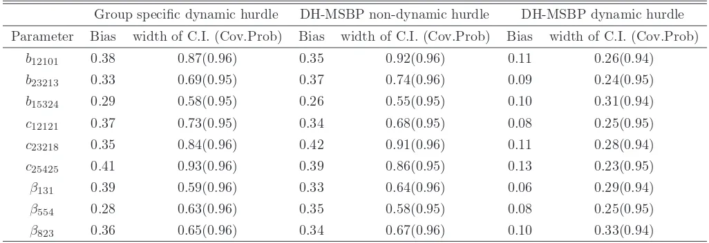
Table 2: Bias, CI width, and CI coverage probability for some of the model parameters in the simulation study.

Group specific dynamic hurdle DH-MSBP non-dynamic hurdle DH-MSBP dynamic hurdle

Parameter Bias width of C.I. (Cov.Prob) Bias width of C.I. (Cov.Prob) Bias width of C.I. (Cov.Prob)

b12101 0.38 0.87(0.96) 0.35 0.92(0.96) 0.11 0.26(0.94)

b23213 0.33 0.69(0.95) 0.37 0.74(0.96) 0.09 0.24(0.95)

b15324 0.29 0.58(0.95) 0.26 0.55(0.95) 0.10 0.31(0.94)

c12121 0.37 0.73(0.95) 0.34 0.68(0.95) 0.08 0.25(0.95)

c23218 0.35 0.84(0.96) 0.42 0.91(0.96) 0.11 0.28(0.94)

c25425 0.41 0.93(0.96) 0.39 0.86(0.95) 0.13 0.23(0.95)

β131 0.39 0.59(0.96) 0.33 0.64(0.96) 0.06 0.29(0.94)

β554 0.28 0.63(0.96) 0.35 0.58(0.95) 0.08 0.25(0.95)

Table 3: Distribution of the average number of hospital admissions depending on the time of the first hospital visits for the HRS data

Waves

Wave for the first visit 1 2 3 4 5 6 7 8 9 10

1 - 0.63 0.90 0.52 0.31 0.18 0.32 0.20 0.28 0.32

2 0 - 0.62 0.40 0.43 0.32 0.28 0.26 0.26 0.38

3 0 0 - 0.57 0.25 0.20 0.18 0.23 0.28 0.27

4 0 0 0 - 0.37 0.19 0.24 0.33 0.21 0.36

5 0 0 0 0 - 0.36 0.22 0.26 0.31 0.27

6 0 0 0 0 0 - 0.38 0.38 0.31 0.41

7 0 0 0 0 0 0 - 0.37 0.34 0.58

8 0 0 0 0 0 0 0 - 0.41 0.42

Table 4: Probit model estimates for all the covariates in the HRS data.

Covariate Parameter Estimate 95% C.I.

Blood pressure 0.013 (-1.48,0.97)

Diabetes 0.052 (-1.68,2.51))

Cancer* 2.58 (1.43, 4.29)

Lung problem 1.02 (-2.19, 2.47)

Heart problem 0.16 (-1.31,2.51)

Stroke* 5.53 (2.33, 8.16)

Arthritis 0.0027 (-0.91,0.85)

Psychological problem 0.74 (-1.84,2.78)

Employment Insurance* 2.92 (0.49,4.56)

Gov. Insurance 1.62 (-2.20, 3.89)

Other Insurance* 2.56 (1.21,5.73)

Smoking 0.08 (-1.29,1.56)

Alcohol Consumption 1.04 (-2.68,3.77)

Gender 0.94 (-2.68,2.09)

Education level 0.46 (-1.49,2.36)

BMI 0.085 (-0.96,1.88)

Total assets* 2.51 (1.44,5.63)

Total debt 1.16 (-2.06,3.89)

Table 5: LASSO estimates for the covariates with time-invariant effects on the response for

the “good” SAH group with k=1, in the HRS data.

Covariate Parameter Estimate 95% C.I.

Blood pressure 0.064 (-1.33,0.87)

Diabetes 0.041 (-2.02,1.76)

Cancer* 4.58 (2.65, 5.93)

Lung problem 1.16 (-0.29, 2.05)

Heart problem* 3.56 (1.32,5.68)

Stroke* 10.32 (7.96, 13.30)

Arthritis 0.29 (-1.31,2.04)

Psychological problem 0.02 (-2.11,1.19)

Employment Insurance 0.18 (-2.74,1.55)

Gov. Insurance 3.63 (-1.49,6.26)

Other Insurance 0.03 (-1.49,1.14)

Smoking 0.05 (-2.79,0.68)

Alcohol Consumption 0.007 (-0.99,1.06)

Gender 0.58 (-3.61,2.47)

Table 6: LASSO estimates for the covariates with time-invariant effects on the response for

the “poor” SAH group with k=4, in the HRS data.

Covariate Parameter Estimate 95% C.I.

Blood pressure* 1.89 (0.84,4.02))

Diabetes 0.67 (-1.54,2.51)

Cancer* 3.88 (1.55, 6.01)

Lung problem* 1.53 (1.03, 2.24)

Heart problem* 2.66 (1.13,5.61)

Stroke* 7.19 (3.36, 9.14)

Arthritis* 1.27 (0.59,3.66)

Psychological problem 0

-Employment Insurance 0.26 (-0.56,0.88)

Gov. Insurance* 2.58 (1.39,4.43)

Other Insurance 0.16 (-1.29,0.94)

Smoking* 1.19 (0.78,2.18)

Alcohol Consumption* 2.34 (1.39,4.11)

Gender 0

-Table 7: LASSO estimates for the covariates with time-invariant effects on the response for

the “excellent” SAH group with k=1, in the HRS data.

Covariate Parameter Estimate 95% C.I.

Blood pressure 0.53 (-2.15,1.73)

Diabetes 0.72 (-1.95,1.23))

Cancer* 5.91 (3.50, 6.99)

Lung problem 1.13 (-2.05, 2.86)

Heart problem* 2.54 (1.12,4.65)

Stroke* 8.11 (5.84, 10.71)

Arthritis 0

-Psychological problem 0

-Employment Insurance 0.31 (-0.94,0.75)

Gov. Insurance 0

-Other Insurance 0.83 (-1.04,1.88)

Smoking* 1.59 (0.96,3.18)

Alcohol Consumption 0.06 (-0.39,0.51)

Gender 0

0 500 1000 1500 2000 2500

1 2 3 4 5 6 7 8 9 10 Wave Counts Zero hospitalization 0 100 200

1 2 3 4 5 6 7 8 9 10

Wave

Counts

One time hospitalization

0 25 50 75

1 2 3 4 5 6 7 8 9 10

Wave

Counts

Two times hospitalizations

Wave No. 1 2 3 4 5 6 7 8 9 10 0 10 20 30

1 2 3 4 5 6 7 8 9 10

Wave

Counts

Three times hospitalizations

0.0 2.5 5.0 7.5 10.0 12.5

1 2 3 4 5 6 7 8 9 10 Wave

Counts

Four times hospitalizations

0 1 2 3 4 5

1 2 3 4 5 6 7 8 9 10

Wave

Counts

Five times hospitalizations

Wave No. 1 2 3 4 5 6 7 8 9 10

0.00 0.25 0.50 0.75

0 1 2 3 4 5

No of times Hospitalizations

Density

Health Status 1. excellent 2. very good 3. good 4. fair 5. poor

Self Reported Health Status Vs Times hospitalized

1 2 3 4 5 6 7 8 9 10 0

1 2 3 4 5 6

Wave

Effect of BMI on hospital visits

Fair Poor Very Good Good Excellent

1 2 3 4 5 6 7 8 9 10 0

1 2 3 4 5 6

Wave

Effect of BMI on hospital visits

Fair Poor Very Good Good Excellent

1 2 3 4 5 6 7 8 9 10 0

1 2 3 4 5 6

Wave

Effect of BMI on hospital visits

Fair Poor Very Good Good Excellent

1 2 3 4 5 6 7 8 9 10 0

1 2 3 4 5 6

Wave

Effect of total assets on hospital visits

Fair Poor Very Good Good Excellent

1 2 3 4 5 6 7 8 9 10 0

1 2 3 4 5 6

Wave

Effect of total assets on hospital visits

Fair Poor Very Good Good Excellent

1 2 3 4 5 6 7 8 9 10 0

1 2 3 4 5 6

Wave

Effect of total assets on hospital visits

Fair Poor Very Good Good Excellent

Figure 4: Time varying effect of the total assets for 5 different groups for k=2, 4 and 6

1 2 3 4 5 6 7 8 9 10 0

1 2 3 4 5 6

Wave

Effect of total debt on hospital visits

Fair Poor Very Good Good Excellent

1 2 3 4 5 6 7 8 9 10 0

1 2 3 4 5 6

Wave

Effect of total debt on hospital visits

Fair Poor Very Good Good Excellent

1 2 3 4 5 6 7 8 9 10 0

1 2 3 4 5 6

Wave

Effect of total debt on hospital visits

Fair Poor Very Good Good Excellent

Figure 5: Time varying effect of the total debt for 5 different groups for k=2, 4 and 6

1 2 3 4 5 6 7 8 9 10 0

1 2 3 4 5 6

Wave

Effect of household income on hospital visits

Fair Poor Very Good Good Excellent

1 2 3 4 5 6 7 8 9 10 0

1 2 3 4 5 6

Wave

Effect of household income on hospital visits

Fair Poor Very Good Good Excellent

1 2 3 4 5 6 7 8 9 10 0

1 2 3 4 5 6

Wave

Effect of household income on hospital visits

Fair Poor Very Good Good Excellent

Figure 6: Time varying effect of the total household income for 5 different groups for k=2,

Web-Appendix

Simulation Study Details and Additional HRS Data Graphs

We simulate data on 100 individuals belonging to 4 related groups at 10 different time

points. Our response is a count variable and we consider 2 continuous predictors with

time-varying effects on the response; and 10 predictors with time-invariant effects. Among the

predictors with time-invariant effects, there are 8 continuous predictors, and the remaining

2 are categorical in nature.

Let x be the set of all covariates; thus x = [x1, x2, . . . , x12]T. Again, for each predictor

xi, we have measurements for T = 10 time points. Hence, xi = [xi(1), xi(2), . . . , xi(10)]T.

We simulate the predictors xis, for i = 1,2, . . . ,10, from a multivariate normal density

with mean=µ₁ = [1,3,5,4,5,6,3.5,5.5,6,3.8]T_{, and covariance matrix=Σ, which is the first}

order auto-regressive structure with ρ1 = 0.65 andσ2 = 3.6. The predictors x11 and x12 are

generated at each time point from Bernoulli distributions withp=0.46 and 0.55, respectively.

Next, we generate πirt, the probabilities of non-zero response. We first generate the

iid samples of (ηi, bi) from a bivariate normal density with mean vector=0 and

covari-ance matrix=

10 5.01

− 8.6

.Then the probabilities πirtare generated from the following probit

model:

πirt = Φ(xTi δ+ηi), withδ= [0.04,1.4,2.5,0.005,3.6,6.3,−2.56,0.02,−0.003,4.36,1.1,−3.9]T.

For each individual i, at each time pointt, we sample from a uniform (0,1) distribution; and

assign a zero value with probability=1-πirt. Note that individuals change their groups as

described in Section 4 of the main text.

Next, for each individuali, we find the time corresponding to the first non-zero response.

Ift is that time, then we generate Ti, the exact time of the first hospital visit for individual

i. We generate Ti from a Weibull (1,5) distribution truncated below at t−1 and truncated

above by t. Next, we sample Yirt for each individual at each time point t as follows.

For the i-th individual, if t is the time for the first non-zero response, then we sample

Yirt from the distribution given in equation (2) of the main text, and if t is the time after

the first non-zero response, then we sample Yirt using the model given in equation (3) of

the main text, with k = 0,1, . . . ,5. We consider x1 and x2 as the predictors with

time-varying effects on the response, while the other 10 predictors are treated as the covariates

with time-invariant effects on the response. Thus, we have J = 2 and J0 = 10.

Next, we specify the parameter values for the model in equation (3). For our simulation,

we take βj0_kr =β_j0, and consider β = [2.3,4.5,3.9,0.04,6.1,3.2,0.003,−1.65,−0.06,1.4]. For

the time-varying part, we consider gj=2, for j = 1,2 and two knots at at time 3 and 7,

thus Sj = 2. Define bjkrt = [bjkr0t, bjkr1t, bjkr2t]T, and also cjkrt = [cjkr1t, cjkr2t]T. We show

the parameter values for our simulation study for different choices of k and j. We present

selected tables below: the other findings were very similar and, hence, for brevity we do not

present them here (they are available on request). Note that the set of parameters for both

b andc are shared across the groups and times for different values ofk and j, thus allowing

a shared parameter structure.

Table S.1: Model parameter values for bjkrt across groups and times forj=1 andk = 1.

Time Group 1 Group 2 Group 3 Group 4

1 (1.74,0.86,1.31) (1.71,0.82,1.24) (1.80,0.91,1.31) (1.75,0.86,1.34)

2 (1.69,0.85,1.42) (1.80,0.73,1.26) (1.63,0.81,1.19) (1.77,0.81,1.34)

3 (1.82,0.93,1.24) (1.77,0.79,1.14) (1.69,0.76,1.24) (1.72,0.88,1.30)

4 (1.77,0.88,1.37) (1.76,0.81,1.37) (1.76, 1.02,1.41) (1.80,0.81,1.38)

5 (1.65,0.78,1.30) (1.69,0.86,1.42) (1.79,0.87,1.26) (1.71,0.87,1.36)

6 (1.73,0.84,1.28) (1.75,0.84,1.28) (1.92,0.93,1.33) (1.80,0.88,1.33)

7 (1.81,0.89,1.32) (1.68,0.97,1.21) (2.05,0.77,1.37) (1.76,0.91,1.35)

8 (1.66,0.73,1.25) (1.94,0.82,1.04) (1.78,0.75,1.30) (1.69,0.74,1.25)

9 (1.76,0.75,1.28) (1.84,0.82,1.24) (1.77,0.79,1.30) (1.70,0.81,1.35)

10 (1.75,0.78,1.33) (1.88,0.82,1.34) (1.84,0.85,1.32) (1.80,0.81,1.37)

Table S.2: Model parameter values for bjkrt across groups and times forj=1 andk = 5.

Time Group 1 Group 2 Group 3 Group 4

1 (1.84,0.89,1.26) (1.73,0.87,1.34) (1.80,0.91,1.31) (1.85,0.91,1.24)

2 (1.68,0.86,1.44) (1.85,0.76,1.27) (1.69,0.89,1.10) (1.71,0.82,1.33)

3 (1.77,0.91,1.34) (1.75,0.81,1.24) (1.66,0.86,1.32) (1.75,0.83,1.31)

4 (1.71,0.82,1.33) (1.74,0.95,1.36) (1.77, 1.08,1.49) (1.80,0.86,1.34)

5 (1.75,0.78,1.30) (1.63,0.84,1.44) (1.69,0.87,1.31) (1.74,0.88,1.32)

6 (1.73,0.86,1.23) (1.77,0.88,1.38) (1.82,0.83,1.23) (1.80,0.78,1.43)

7 (1.81,0.89,1.32) (1.78,0.87,1.21) (2.01,0.77,1.27) (1.76,0.81,1.25)

8 (1.86,0.73,1.29) (1.94,0.84,1.44) (1.76,0.85,1.31) (1.79,0.84,1.25)

9 (1.71,0.75,1.28) (1.86,0.82,1.24) (1.87,0.79,1.30) (1.70,0.86,1.43)

10 (1.69,0.78,1.43) (1.98,0.91,1.34) (1.85,0.88,1.34) (1.77,0.86,1.39)

Table S.3: Model parameter values for bjkrt across groups and times forj=2 andk = 2.

Time Group 1 Group 2 Group 3 Group 4

1 (1.54,0.66,1.41) (1.51,0.62,1.44) (1.70,0.61,1.36) (1.65,0.66,1.34)

2 (1.49,0.55,1.42) (1.60,0.71,1.36) (1.63,0.51,1.29) (1.67,0.71,1.31)

3 (1.62,0.63,1.34) (1.57,0.69,1.44) (1.69,0.56,1.34) (1.62,0.68,1.30)

4 (1.77,0.89,1.47) (1.66,0.61,1.37) (1.76, 1.02,1.31) (1.70,0.71,1.28)

5 (1.75,0.88,1.50) (1.69,0.66,1.32) (1.79,0.97,1.26) (1.61,0.77,1.36)

6 (1.73,0.85,1.38) (1.65,0.74,1.38) (1.92,0.93,1.33) (1.80,0.78,1.43)

7 (1.81,0.89,1.32) (1.69,0.97,1.21) (1.95,0.87,1.35) (1.76,0.87,1.35)

8 (1.86,0.93,1.35) (1.94,0.92,1.24) (1.78,0.75,1.30) (1.69,0.74,1.35)

9 (1.86,0.85,1.38) (1.94,0.91,1.34) (1.75,0.75,1.27) (1.80,0.84,1.45)

10 (1.75,0.78,1.33) (1.78,0.82,1.34) (1.74,0.85,1.32) (1.70,0.71,1.30)

Table S.4: Model parameter values for bjkrt across groups and times forj=2 andk = 4.

Time Group 1 Group 2 Group 3 Group 4

1 (1.64,0.79,1.46) (1.63,0.81,1.39) (1.70,0.84,1.36) (1.75,0.91,1.44)

2 (1.68,0.76,1.44) (1.65,0.76,1.37) (1.69,0.89,1.20) (1.71,0.92,1.43)

3 (1.67,0.81,1.35) (1.75,0.81,1.34) (1.76,0.86,1.32) (1.65,0.81,1.46)

4 (1.74,0.72,1.33) (1.64,0.75,1.36) (1.77, 1.01,1.39) (1.80,0.86,1.34)

5 (1.75,0.78,1.30) (1.63,0.84,1.34) (1.69,0.87,1.31) (1.74,0.84,1.32)

6 (1.63,0.86,1.33) (1.67,0.88,1.38) (1.72,0.83,1.33) (1.70,0.78,1.36)

7 (1.71,0.79,1.32) (1.78,0.77,1.31) (2.01,0.77,1.27) (1.76,0.81,1.35)

8 (1.66,0.73,1.29) (1.64,0.74,1.34) (1.77,0.85,1.31) (1.71,0.74,1.25)

9 (1.71,0.75,1.28) (1.66,0.82,1.24) (1.77,0.79,1.30) (1.70,0.76,1.33)

10 (1.69,0.78,1.33) (1.68,0.81,1.34) (1.85,0.88,1.34) (1.77,0.76,1.31)

Table S.5: Model parameter values for cjkrt across groups and times forj=1 andk=1.

Time Group 1 Group 2 Group 3 Group 4

1 (0.74,0.96) (0.77,0.98) (0.79,0.95) (0.81,0.95)

2 (0.79,0.92) (0.72,0.95) (0.71,0.91) (0.76,0.92)

3 (0.81,1.01) (0.79,0.91) (0.76,0.94) (0.77,0.88)

4 (0.77,0.94) (0.70,0.93) (0.72,0.97) (0.79,0.89)

5 (0.74,0.95) (0.86,0.99) (0.83,0.90) (0.74,0.84)

6 (0.75,0.99) (0.67,0.91) (0.73,0.99) (0.76,0.95)

7 (0.68,0.89) (0.75,0.97) (0.69,0.92) (0.69,0.86)

8 (0.64,0.88) (0.74,0.92) (0.68,1.12) (0.69,0.87)

9 (0.73,0.84) (0.74,0.96) (0.66,0.86) (0.79,0.95)

10 (0.74,0.88) (0.74,0.82) (0.68,1.02) (0.69,0.88)

Table S.6: Model parameter values for cjkrt across groups and times forj=1 andk=5.

Time Group 1 Group 2 Group 3 Group 4

1 (0.64,0.75) (0.67,0.73) (0.59,0.71) (0.61,0.75)

2 (0.69,0.72) (0.62,0.75) (0.61,0.71) (0.66,0.72)

3 (0.71,0.81) (0.68,0.71) (0.56,0.70) (0.67,0.78)

4 (0.67,0.74) (0.60,0.73) (0.62,0.77) (0.69,0.79)

5 (0.64,0.75) (0.76,0.75) (0.63,0.70) (0.64,0.74)

6 (0.65,0.79) (0.57,0.71) (0.63,0.79) (0.66,0.75)

7 (0.58,0.79) (0.65,0.77) (0.59,0.72) (0.65,0.76)

8 (0.54,0.68) (0.64,0.70) (0.58,0.81) (0.69,0.79)

9 (0.63,0.64) (0.64,0.76) (0.66,0.76) (0.63,0.75)

10 (0.64,0.78) (0.64,0.72) (0.68,0.77) (0.61,0.78)

Table S.7: Model parameter values for cjkrt across groups and times forj=2 andk=4.

Time Group 1 Group 2 Group 3 Group 4

1 (0.45,0.55) (0.47,0.53) (0.39,0.51) (0.41,0.55)

2 (0.49,0.52) (0.42,0.55) (0.41,0.49) (0.36,0.52)

3 (0.41,0.51) (0.38,0.51) (0.46,0.50) (0.37,0.48)

4 (0.47,0.54) (0.40,0.53) (0.42,0.47) (0.39,0.49)

5 (0.44,0.55) (0.46,0.55) (0.43,0.50) (0.44,0.54)

6 (0.45,0.49) (0.47,0.51) (0.43,0.49) (0.46,0.55)

7 (0.38,0.59) (0.45,0.57) (0.39,0.52) (0.45,0.56)

8 (0.44,0.48) (0.44,0.50) (0.38,0.51) (0.39,0.49)

9 (0.66,0.84) (0.64,0.86) (0.66,0.85) (0.63,0.80)

10 (0.72,0.68) (0.74,0.82) (0.78,0.87) (0.81,0.79)

1 2 3 4 5 6 7 8 9 10

1. excellent 2. very good 3. good 4. fair 5. poor

Health Status

W

a

v

e

Avg. Hosp.

0.5

1.0

1.5

Average number of times hospitalization

Figure S.1: Heat map displaying the average number of hospitalizations across different waves and self reported health status.

0 500 1000 1500 2000 2500

0 1 2 3 4 5

No of times Hospitalizations

No

. of P

eople

Wave No.

1 2 3 4 5 6 7 8 9 10

No. of people Vs Times hospitalized

Figure S.2: Plot showing the distribution of individuals across the number of hospitalizations for different waves.