A comparison of some numerical methods for the advection diffusion equation

(1)

A Comparison of Some Numerical

Methods for the Advection-Diffusion

Equation

M. Thongmoon 1 & R. McKibbin2

1_{King Mongkut’s University of Technology Thonburi, Thailand}

[email protected]

2_{Institute of Information and Mathematical Sciences}

Massey University at Albany, Auckland, New Zealand

[email protected]

This paper describes a comparison of some numerical methods for solving the advection-diffusion (AD) equation which may be used to describe transport of a pollutant. The one-dimensional advection-diffusion equation is solved by using cubic splines (the natural cubic spline and a ”special” AD cubic spline) to estimate first and second derivatives, and also by solving the same problem using two standard finite difference schemes (the FTCS and Crank-Nicolson methods). Two examples are used for comparison; the numerical results are compared with analytical solutions. It is found that, for the examples studied, the finite difference methods give better point-wise solutions than the spline methods.

1 Introduction

Pepper et al. (1) and Okamoto et al. (2) solve the one-dimensional advection equa-tion by using a spline interpolaequa-tion technique that they call a quasi-Lagrangian cubic spline method. In section 4 of (3), Ahmad & Kothyari solve the one dimensional advection-diffusion equation by using cubic spline interpolation for the advection component and the Crank-Nicolson scheme for the diffusion component. Sastry (6) uses a cubic spline technique to approximate the solution of the one-dimensional diffusion equation.

(2)

2 Governing Equation and Numerical Methods

2.1 Governing Equation

The volumetric concentration of a pollutant in a moving, turbulent fluid may be described by the advection-diffusion equation

∂C

∂t +∇·(VC) =∇ ·( ¯K⊗ ∇C) (1)

Here, C(x, y, z, t) is the concentration (mass per unit volume) of pollutant at point (x, y, z) in Cartesian coordinates, at timet. The vector V _{is the fluid velocity field} and ¯K is the eddy-diffusivity or dispersion tensor.

In this study, we consider one-dimensional motion with constant speed u and dispersionD which gives the 1-D advection-diffusion equation:

∂C ∂t +u

∂C ∂x =D

∂2_C

∂x2 (2)

with appropriate initial and boundary conditions. Here,C(x, t) is the concentration of the pollutant at point x (0_≤ x _≤ L) and time t, u is the constant wind speed in the x direction and D is the diffusivity coefficient in the x direction. Several combinations of boundary conditions are possible. We distinguish three cases, all for a finite domain:

Case 1:

C(x,0) = f(x)

C(0, t) = c0

C(L, t) = cL

(3)

Case 2:

C(x,0) = f(x)

C(0, t) = c0

∂C

∂x(0, t) = 0

(4)

Case 3:

C(x,0) = f(x)

C(0, t) = c0

q(0, t) = (Cu₋D∂C

∂x)(0, t) = constant

(5)

where c0, cL are constant concentration values, while the quantity q = uC−D∂C_∂x

is the mass flux of pollutant per unit cross-sectional area, and includes both of the advective and dispersive components. All cases correspond to a fixed constant con-centration at the left-hand end, together with one of: a constant concon-centration at the right-hand end (Case 1), advective pollutant inflow only at the left-hand end (Case 2) or fixed constant pollutant influx there (Case 3).

For construction of interpolating cubic splines at any step in a numerical approx-imation procedure, 2 extra conditions are required apart from the Ci values at the

mesh points xi. The ”natural” cubic spline requires the condition that ∂

2_C

(3)

the interpolants at x = 0, L. How does this requirement impact on the boundary conditions?

For all cases above,C =c0 at x= 0 implies that

∂C

∂t (0, t) = 0,

and therefore

u∂C ∂x −D

∂2_C

∂x2 = 0

at x = 0, i.e. ∂q_∂x(0, t) = 0. This implies that q(0−

, t) = q(0+_{, t}_{). Assuming that}

the pollutant source is well-mixed, then C = c0 upstream and q = uc0 at x = 0 −

. Because C = c0 at x = 0+, this means that ∂C_∂x = 0 at x = 0+ and so ∂

2_C

∂x2 = 0 at

x= 0+_{. Cases 1 and 2 therefore are consistent with the boundary condition at}_x_{= 0}

corresponding to the natural cubic spline, while Case 3 is not. Hence the motivation for developing a ”special” cubic spline scheme for the advection-dispersion equation, as outlined in a letter section of this paper.

2.2 Finite difference (FTCS) method

Finite difference schemes involve calculating approximate values of the unknown function at a finite number of (mesh- or grid-) points in the domain. Here we let 0 = x1 ≤ xj ≤ xN+1 = L be the grid points in x-domain. The time is divided into

equal steps of size ∆t, with timetn−n∆t. Derivatives are approximated by truncated

Taylor Series expansions. For our purposes, we use an explicit forward difference estimate for the time derivative (FT), and central difference approximations for the space derivatives (CS) that both have the same truncation error; hence the acronym FTCS. The approximate solution of the governing equation using the finite difference scheme satisfies:

Cjn+1−Cjn

∆t +u Cn

j+1−Cjn−₁

2∆x =D Cn

j+1−2Cjn+Cjn−₁

(∆x)2 +O(∆t,(∆x)

2₎ ₍₆₎

for j = 2,3, . . . , N, while for j =N + 1, one-sided forms of the difference formulae are required:

C_Nn+1₊₁−Cn N+1

∆t +u

3Cn N+1−4C

n N+CNn−1

2∆x

=D2CNn+1−5C

n N+4C

n N−1

−Cn N−2

(∆x)2 +O(∆t,(∆x)2)

(7)

all for for n= 0,1,2, . . ., where the initial values are C0

j =C((j −1)∆x,0).

Hindmarsh (7) and Sousa (8), show that the conditions that the finite difference scheme in Equation (6) is stable are

(4)

and

(u∆t ∆x)

2

≤2D∆t ∆x2.

Rearrangement and simplification of both of these conditions gives the restriction on the size of the time step in terms of the parameters and the grid-size:

∆t_≤min_{∆x

2

2D ,

2D u2 }

2.3 The Crank-Nicolson method

The Crank-Nicolson scheme approximates the governing equation by using central differences in time; the spatial derivatives are estimated by the average of their values at time step n and step n+ 1, in the form:

C_jn+1−Cn j

∆t +u(

1 2(

C_jn₊₁+1−C_jn+1

−1

2∆x +

Cn j+1−C

n j−1

2∆x ))

=D(1 2(

C_jn+1+1−2C

n+1

j +C n+1

j−1

(∆x)2 +

Cn

j+1−2Cjn+Cjn−1

(∆x)2 )) +O(∆t,∆x2),

(8)

with a similar equation for the right-hand end-point. The Crank-Nicolson scheme is unconditionally stable (4).

2.4 Cubic spline method (”natural” cubic spline)

For this work the definition of the ”natural” cubic spline includes:

(i) The interpolating spline segments are cubic polynomial functions on each sub-interval [xj, xj+1],j = 1,2, . . . , N, and the segments agree with the function values

at the grid-points;

(ii) the first and second derivatives of the cubic spline segments are continuous at the internal points;

(iii) the second derivatives of the cubic spline segments at the first and the last grid points are equal to zero.

The approximate solution of the governing equation using the cubic spline method satisfies:

Cn+1

j −Cjn

∆t +uP n

j =DQnj. (9)

for j = 1,2, . . . , N + 1;n = 0,1,2, . . . where Pn

j is the first derivative and Qnj the

second derivative of the cubic spline function at the pointxj at timen∆t. Equation

(9) can be written in the explicit form:

Cjn+1 =C n

j +D∆tQ n

j −u∆tP n

j . (10)

The values of the slopes Pn

j can be obtained by solving the following system of

(5)

the continuity conditions for the spline segments; see (5) for details of algebraic working):            

2 1 0 0 0 . . . 0 0 0

α2 2 µ2 0 0 . . . 0 0 0

0 α3 2 µ3 0 . . . 0 0 0

. . .

0 0 0 0 0 . . . αN−₁ 2 µN−₁

0 0 0 0 0 . . . 0 1 2

                        Pn 1 Pn 2 Pn 3 . . . Pn N Pn N+1             =             dn 1 dn 2 dn 3 . . . dn N dn N+1             (11) where dn

1 = 3(

Cn

2−C1n

x2−x1 )

dn

i = 3

µj

hj+1(C

n

j+1−Cjn) + 3 αj

hj(C

n

j −Cjn−₁) for j=2,3,. . . ,N

dn

N+1 = 3(

Cn N+1−CNn

xN+1−xN)

and where αj =

hj+1

(hj+hj+1), muj = 1−αj =

hj

(hj+hj+1), hj+1 = xj+1−xj and hj =

xj −xj−₁.

The values of Qn

j are the second derivatives of cubic spline at points xj for j = 2,3, . . . , N, at timen∆t. For the natural cubic spline it is assumed thats′′

1(x1) =

s′′

n(xn+1) = 0 (i.e. Qn1 =QnN+1 = 0). Then we have:

Qn j = 6

Cn

j+1−Cjn

(xj+1−xj)2 −

4 P

n j

xj+1−xj −

2 P

n j+1

xj+1−xj

(12)

for j = 2,3, . . . , N.

2.5 Cubic spline method (”Special A-D” cubic spline)

The boundary condition C=c0 atx= 0, implies that

∂C

∂t (0, t) = 0, (13)

and so

(u∂C ∂x −D

∂2_C

∂x2)(0, t) = 0. (14)

In this section we present a cubic spline interpolation scheme that satisfies the condition (12).

The requirement is that uPn

(6)

Qn

1 = DuP

n

1 and QnN+1 = DuP

n

N+1 (compare with natural cubic spline where Qn1 =

0;Qn

N+1 = 0). The values ofPjn can then be calculated from the following system:

AP =d (15)

where A=            

2 + u(x2−x1)

2D 1 0 0 0 . . . 0 0 0

α2 2 µ2 0 0 . . . 0 0 0

0 α3 2 µ3 0 . . . 0 0 0

. . .

0 0 0 0 0 . . . αn−₁ 2 µn−₁

0 0 0 0 0 . . . 0 1 4D−u(xN+1−xN)

2D             P =             Pn 1 Pn 2 Pn 3 . . . Pn N Pn N+1             and d=             dn 1 dn 2 dn 3 . . . dn N dn N+1             where dn

1 = 3(

Cn

2−Cn1

x2−x1 )

dn

j = 3

µj

hj+1(C

n

j+1−Cjn) + 3 αj

hj(C

n

j −Cjn−₁) for j=2,3,. . . ,N

dn

N+1 = 3(

Cn N+1−CNn

xN+1−xN)

and αj =

hj+1

(hj+hj+1) and µj = 1−αj =

hj

(hj+hj+1). For this case Q

n

j, j = 2,3, . . . , N

can be obtained from

Qn j = 6

Cn

j+1−Cjn

(xj+1−xj)2 −

4 P

n j

(xj+1−xj) −

2 P

n j+1

(xj+1−xj)

(7)

whileQn

1 andQN+1nare calculated directly using the formulae already given above.

3 Numerical Experiments

Two examples are solved by the various methods outlined above, and the calculated numerical approximations are compared with the analytical solutions and with each other. The idea is to try to find the method which gives the best estimates for solu-tions of the advection-dispersion equation. Example 1 is a boundary value problem on a finite domain, as in Case 1 defined in Section 2.1 above. Example 2 is for a semi-infinite domain, but a finite-domain solution is sought.

3.1 Example 1.

The one-dimensional advection-diffusion equation:

∂C ∂t +u

∂C ∂x =D

∂2_C

∂x2 (17)

is to be solved with the boundary and initial conditions:

C(0, t) = 0

C(L, t) = 100

C(x,0) = 100x

L 0≤x≤L

The analytical solution is (4):

C(x, t) = 100[ e

P x L −1

eP ₋₁ +

4πeP x2Lsinh(P/2)

eP ₋₁

∞

X

m=1

Am+ 2πe

P x

2L

∞

X

m=1

Bm] (18)

where P is the Peclet number

P = uL

D

and the coefficients Am, Bm are given by

Am = (−1)m m βm

sin(mπx

L )e

−λmt

Bm = [ (−1)m+1 m βm

(1 + P

βm

)e−P

2 + mP

β2

m

] sin(mπx

L )e

−λmt_,

where

βm = ( P

2)

2_{+ (}_mπ₎2

and

λm = u2

4D +

m2_π2_D

L2 =

Dβm L2

In this study, we assume that L = 1.0 m, D = 0.01 m2_s−₁

, u = 0.1 ms−₁

(8)

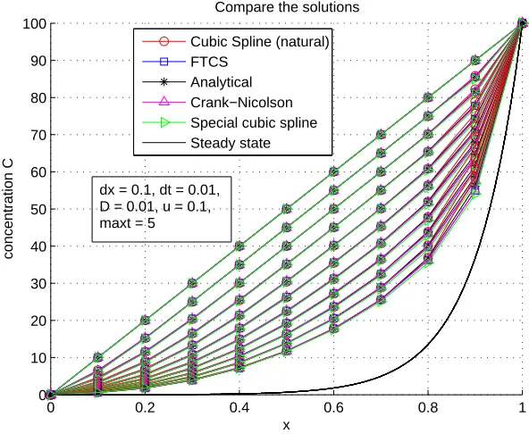
0 0.2 0.4 0.6 0.8 1 0

10 20 30 40 50 60 70 80 90 100

x

concentration C

Compare the solutions

Cubic Spline (natural) FTCS

Analytical Crank−Nicolson Special cubic spline Steady state

[image:8.612.133.429.65.308.2]

dx = 0.1, dt = 0.01, D = 0.01, u = 0.1, maxt = 5

Figure 1: Comparisons of the solutions for Example 1 using various methods

It can be seen in Figure 1 that the numerical solutions given by all of the methods decrease with time from the initial (linear profile) condition. The calculated values are shown at times t = 0(0.5)5s. The time T = 5s is still too early for the steady state to be approached. The errors in the numerical results are shown in Figure 2.

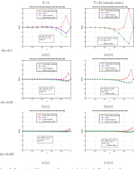
Figure 2 shows the error in the numerical solutions from each of the methods when compared with the analytical solution, for the three casesN = 10, N = 20 and

N = 40, corresponding to ∆x = 0.1,0.05 and 0.025 respectively. Comparisons are made for the solutions at timet= 5sandt = 25s. The latter time corresponds very closely to steady state. From Figure 2(a)(i) forT = 5 and ∆x= 0.1, the errors are all small except near x = 1. The error for the natural cubic spline is positive and larger in magnitude than the errors for the other three methods, which are all negative. For smaller ∆x [in (b)(i)∆x = 0.05 and (c)(i)∆x = 0.025] the errors all reduce in size and appear to be _O(∆x2_).

(9)

T=5 T=25 (steady-state)

dx=0.1

0 0.2 0.4 0.6 0.8 1

−4 −3 −2 −1 0 1 2 3 4 x Error

The error of numerical method at the last time step

Crank−Nicolson Special cubic spline

dx = 0.1, dt = 0.01, D = 0.01, u = 0.1, maxt = 5

0 0.2 0.4 0.6 0.8 1

−4 −3 −2 −1 0 1 2 3 4 x Error

dx = 0.1, dt = 0.01, D = 0.01, u = 0.1, maxt = 25

(steady−state)

(a)(i) (a)(ii)

dx=0.05

0 0.2 0.4 0.6 0.8 1

−4 −3 −2 −1 0 1 2 3 4 x Error

dx = 0.05, dt = 0.01, D = 0.01, u = 0.1, maxt = 5

0 0.2 0.4 0.6 0.8 1

−4 −3 −2 −1 0 1 2 3 4 x Error

dx = 0.05, dt = 0.01, D = 0.01, u = 0.1, maxt = 25 (steady−state)

(b)(i) (b)(ii)

dx=0.025

0 0.2 0.4 0.6 0.8 1

−4 −3 −2 −1 0 1 2 3 4 x Error

dx = 0.025, dt = 0.01 D = 0.01, u = 0.1, maxt = 5

0 0.2 0.4 0.6 0.8 1

−4 −3 −2 −1 0 1 2 3 4 x Error

dx = 0.025, dt = 0.01, D = 0.01, u =0.1, maxt = 25 (steady−state)

[image:9.612.106.573.57.639.2]

(c)(i) (c)(ii)

(10)

Because the solutions of the FTCS and Crank-Nicolson methods give better point-wise approximations to the analytical solutions than the ”natural” cubic spline and ”Special A-D” cubic spline schemes for Example 1, for the next example we will present only the solutions given by the FTCS method and the natural cubic spline schemes.

3.2 Example 2.

Solve the one-dimensional advection-diffusion equation:

∂C ∂t +u

∂C ∂x =D

∂2_C

∂x2 (19)

on a semi-infinite domain x= [0,_∞), with the initial and boundary conditions:

C(x,0) = 0 ;x_≥0

C(0, t) = 1 ;t >0

∂C(∞,t)

∂x = 0 ;t >0.

The analytical solution to this problem is given by (9):

C(x, t) = 1 2[erf c(

x₋ut √

4Dt) + exp( xu

D)erf c( x+ut √

4Dt)]

where erf c(x) is the complementary error function defined by

erf c(x) = 1₋erf(x)

where

erf(x) = _√2

π

Z x

0

e−_z2

dz

In this example, the solution is required for a semi-infinite domain but we will solve this problem over a finite domain x = [0,2] by assuming that L = 2 m, D = 0.01 m2_s−₁

, u = 0.1 ms−₁

,∆x = 0.1 m (i.e. N = 20) and ∆t = 0.01 s. We will then comparer the solutions for 0_≤x_≤1 only.

In this example the special cubic spline method is not presented. The conditions for a specialized A-D cubic spline method for this example are Pn

1 = 0 and Qn1 = 0,

which are different from the conditions for the ”Special A-D” cubic spline in Example 1.

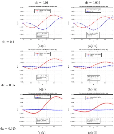
The numerical solutions and the analytical solution for this example may be compared in Figure 3. Figure 4 shows the error of the numerical solutions when compared with the analytical solution, for the two cases N = 10 and N = 40, respectively. The values in Figure 4 are plotted every 50 time steps [i.e. at t = 0(0.05)5s].

(11)

0 0.5 1 1.5 2 −0.2

0 0.2 0.4 0.6 0.8 1 1.2

x

Concentration C

Solutions

Natural Cubic Spline FTCS

Analytical

[image:11.612.138.474.214.491.2]

dx = 0.1, dt = 0.01, D = 0.01, u = 0.1, maxt = 5

(12)

dt = 0.01 dt = 0.005

dx = 0.1

0 0.2 0.4 0.6 0.8 1

References

[1] D.W. Pepper, C.D. Kern and P.E. Long, Jr. Modeling the dispersion of atmo-spheric pollution using cubic splines and chapeau functions. Atmos. Environ.,13, 1979, 223-237.
[2] S. Okamoto, K. Sakai, K. Matsumoto, K. Horiuchi and K. Kobayashi. Devel-opment and application of a three-Dimensional Taylor-Galerkin numerical model for air quality simulation near roadway tunnel portals.J. Appl. Meteor.,37,1998, 1010-1025.
[3] Z. Ahmad and U.C. Kothyari. Time-line cubic spline interpolation scheme for solution of advection equation. Computer & Fluids,30, 2001, 737-752.
[5] E.V. Shikin and A.I. Plis. Handbook on splines for the user. CRC Press Inc. 1995.
[6] S.S. Sastry. Finite difference approximations to one-dimensional parabolic equa-tions using a cubic spline technique. J. Comp. Appl. Math., 2, 1976.
[7] A.C. Hindmarsh, P.M. Gresho and D.F. Griffiths. The stability of explicit Euler time-integration for certain finite difference approximations of the multi-dimensional advection-diffusion equation. Int. J. Numer. Methods Fluids,4, 853-897, 1984.
[8] E. Sousa, The controversial stability analysis. Applied Mathematics and
Com-putation,145, 777-794, 2003.