Edited by:
Letizia Tedesco, Finnish Environment Institute (SYKE), Finland
Reviewed by:
Urania Christaki, Université du Littoral Côte d’Opale, France Kevin Arrigo, Stanford University, United States Maria A. Van Leeuwe, University of Groningen, Netherlands
*Correspondence:
Mar Fernández-Méndez mar.fdez.mendez@gmail.com; mar@npolar.no
Specialty section:
This article was submitted to Marine Ecosystem Ecology, a section of the journal Frontiers in Marine Science
Received:15 July 2017
Accepted:20 February 2018
Published:12 March 2018
Citation:
Fernández-Méndez M, Olsen LM, Kauko HM, Meyer A, Rösel A, Merkouriadi I, Mundy CJ, Ehn JK, Johansson AM, Wagner PM, Ervik Å, Sorrell BK, Duarte P, Wold A, Hop H and Assmy P (2018) Algal Hot Spots in a Changing Arctic Ocean: Sea-Ice Ridges and the Snow-Ice Interface. Front. Mar. Sci. 5:75. doi: 10.3389/fmars.2018.00075
Algal Hot Spots in a Changing Arctic
Ocean: Sea-Ice Ridges and the
Snow-Ice Interface
Mar Fernández-Méndez1*, Lasse M. Olsen1, Hanna M. Kauko1, Amelie Meyer1,
Anja Rösel1, Ioanna Merkouriadi1, Christopher J. Mundy2, Jens K. Ehn2,
A. Malin Johansson3, Penelope M. Wagner4, Åse Ervik5,6, Brian K. Sorrell7, Pedro Duarte1,
Anette Wold1, Haakon Hop1,8and Philipp Assmy1
1Norwegian Polar Institute, Fram Centre, Tromsø, Norway,2Centre for Earth Observation Science, University of Manitoba,
Winnipeg, MB, Canada,3Department of Physics and Technology, UiT The Arctic University of Norway, Tromsø, Norway, 4Norwegian Ice Service, Norwegian Meteorological Institute, Tromsø, Norway,5Sustainable Arctic Marine and Coastal
Technology, Centre for Research-based Innovation, Norwegian University of Science and Technology, Trondheim, Norway,
6The University Centre in Svalbard, Longyearbyen, Norway,7Department of Bioscience, Aarhus University, Aarhus, Denmark, 8Department of Arctic and Marine Biology, Faculty of Biosciences, Fisheries and Economics, UiT The Arctic University of
Norway, Tromsø, Norway
During the N-ICE2015 drift expedition north-west of Svalbard, we observed the establishment and development of algal communities in first-year ice (FYI) ridges and at the snow-ice interface. Despite some indications of being hot spots for biological activity, ridges are under-studied largely because they are complex structures that are difficult to sample. Snow infiltration communities can grow at the snow-ice interface when flooded. They have been commonly observed in the Antarctic, but rarely in the Arctic, where flooding is less common mainly due to a lower snow-to-ice thickness ratio. Combining biomass measurements and algal community analysis with under-ice irradiance and current measurements as well as light modeling, we comprehensively describe these two algal habitats in an Arctic pack ice environment. High biomass accumulation in ridges was facilitated by complex surfaces for algal deposition and attachment, increased light availability, and protection against strong under-ice currents. Notably, specific locations within the ridges were found to host distinct ice algal communities. The pennate diatoms
Nitzschia frigida and Navicula species dominated the underside and inclined walls of submerged ice blocks, while the centric diatom Shionodiscus bioculatus dominated the top surfaces of the submerged ice blocks. Higher light levels than those in and below the sea ice, low mesozooplankton grazing, and physical concentration likely contributed to the high algal biomass at the snow-ice interface. These snow infiltration
communities were dominated by Phaeocystis pouchetii and chain-forming pelagic
diatoms (Fragilariopsis oceanicaandChaetoceros gelidus). Ridges are likely to form more frequently in a thinner and more dynamic ice pack, while the predicted increase in Arctic precipitation in some regions in combination with the thinning Arctic icescape might lead to larger areas of sea ice with negative freeboard and subsequent flooding during the melt season. Therefore, these two habitats are likely to become increasingly important in the new Arctic with implications for carbon export and transfer in the ice-associated ecosystem.
INTRODUCTION
Current changes in sea-ice conditions have consequences for algal biomass and growth, with bottom-up cascading effects on the Arctic marine food web (Wassmann et al., 2011). The significant decline in sea-ice extent and thickness during the last 30 years has caused an increase in the light available for phytoplankton (Arrigo and van Dijken, 2011; Bélanger et al., 2013) and, thus, an increase in phytoplankton net annual primary production (Arrigo and van Dijken, 2015). Likewise, there have been several reports of under-ice phytoplankton blooms in the recent years enabled by the increased light transmission through melt ponds (e.g., Mundy et al., 2009; Arrigo et al., 2012) or through leads (Assmy et al., 2017). In contrast, ice algal areal production is probably decreasing on a pan-Arctic scale due to the loss of sea-ice habitat (Dupont, 2012). In addition, biomass standing stocks are low in young ice compared to the disappearing older ice, probably limited by recruitment, adding to the reduction in sea-ice algal areal production (Lange et al., 2017a; Olsen et al., 2017). As the ice edge retreats further north each summer, ice algae will be limited to the stratified deep basins of the Central Arctic with more oligotrophic conditions compared to the more productive shelves (Barber et al., 2015). The trend toward earlier ice melt and later ice formation may furthermore cause a mismatch in the timing between primary and secondary producers, diminishing the amount of carbon and energy transferred up the food chain (Søreide et al., 2010; Leu et al., 2011; Ji et al., 2013).
Diatoms typically dominate both the phytoplankton and the sea-ice spring blooms, while flagellates, dinoflagellates, and picoeukaryotes usually dominate in late summer (Tremblay et al., 2009; Moran et al., 2012; van Leeuwe et al., 2018). Some diatom species, such asShionodiscus bioculatus(formerlyThalassiosira
bioculata) (Alverson et al., 2006) and Fragilariopsis cylindrus,
are sea-ice associated and have been observed both in the water column and in the ice (von Quillfeldt, 2000). Other sea-ice specialists such as Nitzschia frigida and Melosira arctica
grow attached to the ice, while Chaetoceros gelidus (formerly
Chaetoceros socialis) (Chamnansinp et al., 2013), Fragilariopsis
oceanicaand the haptophyteP. pouchetiiare typically found in
the water column (Booth and Horner, 1997). Current estimates of algal biomass and production in the ice-covered Arctic Ocean generally include phytoplankton and less often sea-ice algae (Gosselin et al., 1997; Sakshaug et al., 2004). Only recent studies have quantified the contribution of other sea-ice related environments, such as melt ponds (Mundy et al., 2011; Lee et al., 2012; Fernández-Méndez et al., 2015), and other more elusive forms of algal accumulations under the ice such as floating algal aggregates (Assmy et al., 2013; Fernández-Méndez et al., 2014).
There are few observations of ice algae growing in ridges (Syvertsen, 1991; Hegseth, 1992; Legendre et al., 1992) and at the snow-ice interface in the Arctic (Buck et al., 1998; McMinn and Hegseth, 2004; von Quillfeldt et al., 2009). Ridges are known to be hot spots for biological activity since they act as shelters for ice fauna and ice-associated zooplankton (Hop and Pavlova, 2008; Gradinger et al., 2010) and juvenile polar cod (Gulliksen and Lønne, 1989). Ridges have also been recently
identified as locations of high algal biomass using under-water remotely operated vehicles (Lange et al., 2017b). However, due to the sampling challenges that these complex structures pose, algae have only been sampled sporadically. Snow infiltration communities growing at the snow-ice interface, have been widely described for Antarctic pack ice (Horner et al., 1988; Spindler, 1994; Robinson et al., 1997; Kristiansen et al., 1998; Garrison et al., 2003), where they contribute substantially to sea-ice primary production (Arrigo et al., 1997). In the few observations obtained from the Arctic, the dominant species reported are mostly phytoplankton such as P. pouchetii in pack ice north of Svalbard and Svalbard fjords (McMinn and Hegseth, 2004; von Quillfeldt et al., 2009), and unidentified pennate and centric diatoms in Disco Island, Greenland (Buck et al., 1998).
Despite these important observations, algal communities growing in ridges and at the snow-ice interface are understudied in the Arctic. Published studies of these two environments mainly focused on a qualitative assessment of the algal species present (especially in ridges), and the photosynthetic performance of the snow infiltration community in the study byMcMinn and Hegseth (2004). During the Norwegian young sea ICE (N-ICE2015) drift expedition, we followed the evolution of these communities over 6 weeks and were able to characterize the physical-chemical environment in which these algal communities thrive, and we explain why these environments are suitable habitats for Arctic microalgae.
The aim of this study is to characterize sea-ice ridges and snow-ice interfaces as potential habitats and refuges for algae in the Arctic Ocean. In particular, we assess the importance of their biomass compared to adjacent environments, we define the light and nutrient regimes that these communities experience, we assess their photosynthetic activity, and we describe the species present. Furthermore, we discuss the role of these environments for hosting algae in the future Arctic Ocean against the background of the ongoing and predicted changes in the Arctic icescape.
MATERIALS AND METHODS
Sampling
All samples were collected during the N-ICE2015 drift expedition that took place between January and June 2015 in ice-covered waters north-west of Svalbard (Granskog et al., 2016). In total four ice floes were occupied and monitored during the expedition. Data presented in this study were obtained during drifts of Floe 3 and 4 (Figure 1A). Sea-ice algae present in ridges were sampled during the drift of Floe 3 between 10 May and 3 June 2015. Between 10 and 18 May, scuba divers using a slurp gun (modified 3.5 L TridentR suction gun) collected
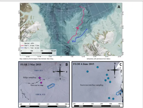
FIGURE 1 | (A)Study area with bathymetry for the N-ICE2015 expedition. The drift trajectories are shown in thick magenta (Floe 3) and blue (Floe 4) lines. The black dotted line indicates the ice edge (>10% ice coverage) position on 25 May 2015. Map created by Max König for the Norwegian Polar Institute. Bathymetry with permission from IBCAO (Jakobsson et al., 2012).(B)Aerial image of the study area during Floe 3 (image taken on 23 May 2015) and location of ridge sampling. The pink line indicates the transect sampled across the ridge and the star the sampling site from which the videos were recorded and the biomass estimates calculated. The pink square indicates the low biomass side of the ridge.(C)Aerial image of the study area during Floe 4 (image taken on 14 June 2015) and locations of snow-ice interface sampling. Vasilii Kustov and Sergey Semenov (Arctic and Antarctic Research Institute. St. Petersburg. Russia).
0.54 m) and used to estimate areal biomass. On 28 May, 31 May and 3 June, sea-ice algae at the ridge were sampled by ice coring with a 9-cm diameter ice corer (Mark II coring system, KOVACS Enterprise, Roseburg, USA). Bottom and top 0.1 m of the cores were collected on 28 May and entire cores of submerged sea-ice ledges were collected in three pieces with the ice corer on 30 May and 3 June for chlorophyll (Chl) a
measurements and quantitative taxonomic analysis at both sides of the ridge. Melting of the ice cores occurred in the dark without addition of filtered seawater to avoid the addition of nutrients.
Algae growing at the snow-ice interface were sampled on Floe 4 between 9 and 18 June. Snow was removed with a shovel to search for brownish coloration as an indicator for algae at random areas with negative freeboard and high snow accumulation. In a radius of 500 m around the ship,
we found and sampled these dense algae accumulations at eight different locations, usually along cracks in the ice (Figures 1C, 3). Samples for qualitative analysis were taken with a snow shovel and melted in clean wide-necked plastic buckets. On 9 June, samples for quantitative analyses were taken using the bottom part of the ice corer and a plastic plate to close the bottom once it was filled with slush.
Characterization of the Physical Setting:
Sea Ice and Snow
[image:3.595.50.550.61.438.2]FIGURE 2 |Scheme of a first-year ice ridge based on observations and measurements performed during May 2015. The square and star correspond to the sampling sites indicated onFigure 1B. The main water current below the ice is a simplification fromFigure 5C. The transmitted irradiance is depicted in a qualitative way to show the reflections that occur inside ridge cavities where the light might be higher than below the ridge itself. The most abundant algal species at the distinct surfaces of the ledges are depicted in the circles to the right based onFigure 3.
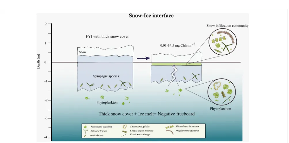
FIGURE 3 |Scheme of snow-ice interface habitat with algal biomass and simplified taxonomic composition. The snow infiltration community is established when thin ice with a thick snow cover starts melting and cracks appear in the ice that enable seawater to infiltrate into the snow-ice slush layer.
was determined by drilling holes with a 0.051 m auger along a transect perpendicular to the ridge length, as described in Ervik et al. (under review). To calculate the ridge macro-porosity (ratio of voids filled with water or slush to the total thickness of the ice)
and 28 May (a compilation of these videos can be found in the Supplementary Material).
Ridge and rubble ice coverage, as well as smooth ice, new ice and open water percentages were assessed from satellite scenes. Five Radarsat-2 scenes of areas located within 10 km of the research vessel’s position from 25 May until 15 June were processed and the percentage of deformed ice was estimated (Table S1, Figure S1). Radarsat-2 scenes use the standard frequency (C-band) for operational sea-ice monitoring and have successfully been used to separate deformed, FYI and multiyear ice (MYI) (Casey et al., 2014). The satellite imagery used here are fully polarimetric scenes with a high spatial resolution (5 m). The scenes were radiometrically calibrated using the included metadata calibration information (MacDonald, 2016), and subsequently segmented using the “extended polarimetric feature space” algorithm (Doulgeris and Eltoft, 2010; Doulgeris, 2013). The segmentation algorithm separated each image into distinct categories based on the statistical properties of the texture features. The identification and classification into open water, new and young ice, smooth ice, and ridges and rubble ice followed procedures used by operational ice analysts and documented in MANICE [Canadian Ice Service (CIS) Meteorological Service of Canada, 2005]. The total percentage of each category type was estimated once the segments had been combined into classified areas.
Water currents below the ice close to the ridge were measured with a medium-range vessel-mounted broadband 150 kHz acoustic Doppler current profiler (ADCP; Teledyne RD Instruments, Poway, CA, USA). Profiles were averaged hourly in 8-m vertical bins with the first bin centered at 23 m (Meyer et al., 2017). Current speed and direction at 23 m depth were used to analyze the current dynamics relative to the ridge during Floe 3 based on the ship’s navigation data. The 23 m depth current data from the vessel-mounted ADCP were the shallowest current data set available for the study time period and were validated by comparing with near surface (1 m depth) current speed available for part of the time period from Acoustic Doppler Velocimeter instruments (ADV; Sontek Xylem, San Diego, CA, USA).
Snow depth and ice thickness on Floe 4 were determined using an electromagnetic instrument (EM31) in combination with a GPS-snow probe as described in Rösel et al. (2018). Negative freeboard areas that could potentially be flooded through cracks in the ice were estimated based on data from snow and ice thickness transects within a radius of 5 km around the ship (Rösel et al., 2016a,b) and drill hole data (Rösel and King, 2017). Additionally, a snow pit was dug and analyzed on 13 June at the first location (SI1) (Figure 1C), where we sampled the snow infiltration communities. Density, temperature, hardness and grain size of the snow were determined at 0.1 m intervals (Gallet et al., 2017).
Light Measurements and Calculations
Transmitted irradiance below ridges was measured during Floe 3 with a vLBV300 remotely operated vehicle (ROV) (SeaBotix.Inc, San Diego, CA, USA). The amount of transmitted photosynthetically active radiation (PAR) available below the studied ridge was measured using a cosine-corrected
hyperspectral irradiance sensor (HyperOCR, Satlantic, Halifax, Canada) mounted on the upper part of the ROV. The same type of sensor was mounted on the surface of the ice looking upwards to measure incoming irradiance. Simultaneous measurements with both sensors allowed for transmittance estimates. In total, 334 radiation measurements at<5 m depth below the ridge were performed during 7, 18, and 20 May. Moreover, based on the observations by divers and the videos from the ROV’s camera (600TVL color), as well as with an underwater camera attached to a pole and deployed through a hole in the ice, we could qualitatively assess the light field inside the ridge.
In addition, we used the following modification of the equation by Light et al. (2008) to calculate light transmitted (PARz) through the ridge with three overlaid ice ledges, separated by voids with water:
PARz = (1−R)×PARsurface×exp[−Ksnow×Zsnow
−Kice×(Zice1+Zice2+Zice3)−Kwater×(Zwater1
+Zwater2)]
where R is the specular reflection that happens at the surface (5%) (Perovich, 1989),PARsurfaceis the incomingPARfrom a Trios-Sensor located at the weather station on the ice camp (Hudson et al., 2016),Ksnow is the snow light attenuation coefficient for PAR (14.82 m−1),Kiceis the ice light attenuation coefficient (0.93
m−1),Kwateris the water light attenuation coefficient (0.1 m−1),
andZis thickness of the three different ledges or the depth of the water voids in between them. The snow attenuation coefficient was calculated from time series of incident and transmittedPAR
and the sea-ice light attenuation coefficient was taken fromLight et al. (2008). To compare with the ROV under-ice measurements, we calculated the light transmitted at the side of the ridge facing the refrozen lead (marked with a star in Figures 1B, 2) from 23 April to 5 June, using its minimum (0.07 m) and maximum (0.11 m) snow depths measured on 28 May. In addition, to obtain an idea of the spatial variability of light transmitted through the ridge, we calculatedPARtransmitted at 1-m intervals where we measured snow depth, ice thickness and water voids on 24 and 31 May.
The amount of light available for the snow infiltration communities was measured with a scalar Mini PAR logger (JFE MKV-L, Japan). In addition, we calculated the transmitted irradiance below 0.2–0.7 m of snow using the measured incoming irradiance and the snow attenuation coefficient mentioned above.
Chemical and Biological Analysis
these high algal biomass environments, it should be measured in future studies. Nutrient concentrations in the water column at 5 m depth are available at the Norwegian Polar Data Centre (Assmy et al., 2016).
For chlorophyll a (Chl a) and particulate organic carbon and nitrogen (POC and PON) 10–200 mL of sample (depending on the coloration of the melted sea-ice sample) were filtered through GFF and pre-combusted GFF filters (diameter 25 mm; Whatman, GE Healthcare, Little Chalfont, UK), respectively. Chl
awas extracted in 5 mL of 100% methanol at 5◦C in the dark for 12 h and measured fluorometrically using a Turner 10-AU Fluorometer (Turner Designs, San Jose, USA). POC and PON samples were analyzed with continuous-flow mass spectrometry (CF-IMRS) using a Roboprep/tracermass mass spectrometer (Europa Scientific, UK).
To calculate the percentage of algal biomass that each environment was contributing to the total sea-ice biomass we multiplied the percentage of surface that each environment (e.g., ridges and deformed ice, deformed edges next to open water or young ice, flooded FYI; non-flooded FYI or second-year ice (SYI) and young ice) covered by the range of biomass measured in each environment.
To calculate nutrient demand we followedCota et al. (1987)
and used our measured Chlaconcentrations, the N:Chlaand Si:Chl a ratios, and the calculated growth rate based on Chl
ameasurements taken over consecutive days. Furthermore, we calculated the nutrient replenishment rate (mmol m−2d−1) by
multiplying the measured nutrient concentrations in the under-ice water (transformed from per cubic meter to per square meter) by the measured water current velocity below the ice.
The physiological status of the photosynthetic apparatus of the algae was assessed with Pulse Amplitude Modulation (PAM) fluorometry using a Phyto-PAM Phytoplankton Analyzer (Walz, Eiffeltrich, Germany). Samples from the ridge were carefully collected by divers every 2 days between 10 and 18 May using a slurp gun, and between 28 and 31 May by scraping the surface of the ice core (the top and the bottom) into filtered seawater. Snow-ice infiltration layer samples for PhytoPAM analysis were collected with a clean bucket on the 9, 10, 11, 13, and 14 June. The quantum yield (8PSII) of photosystem II fluorescence was
determined on 30-min dark-acclimated samples from the ratio of variable and maximal fluorescence (Fv/Fm). In addition, Rapid Light Curves (RLCs) were performed with 20 sec pulses of actinic light ranging between 1 and 900µmol photons m−2 s−1in 13
steps. The relative photosynthetic electron transport rate (rETR) was calculated as the product of8PSII, the theoretical absorption
of PSII and the scalar irradiance of PAR at each pulse. The RLCs were fitted using the equation of Webb et al. (1974) to yield data from which the initial slope (α), the maximum rETR, and the photoacclimation parameter (Ek) were derived. There was no evidence of photoinhibition in any RLCs, so no photoinhibitory modification was included in the model. Only photosynthetic parameters obtained from the blue excitation channel (470 nm) were used, to optimize the signal-to-noise ratio and due to the strong absorption by Chl c, fucoxanthin and carotenoids in blue light by diatoms, which were the dominant algal group in our samples (Walz, 2003; Johnsen and Sakshaug, 2007). To
statistically test for differences in the photosynthetic parameters of the different algal communities in the ridges we used the ANCOVA test for comparison of regression lines; (Sokal and Rohlf, 2012).
An additional approach used to test whether the diatoms found in the ridges and the snow-ice interface were actively growing was the silica stain method (McNair et al., 2015). We added 100 µL of the fluorescent dye 2-(4-pyridyl)-5-((4-(2-dimethylaminoethylaminocarbamoyl) -methoxy)phenyl)oxazole (PDMPO) (1 mM PDMPO in dimethylsulphoxide (DMSO) solution; ThermoFisher Scientific, Waltham, MA, USA) to 70 mL of each sample. After incubating in transparent plastic cell culture bottles in situ for 24 h, the samples were observed and photographed under an inverted Nikon TS100 light microscope (Nikon, Tokyo, Japan) on board. We show a selection of these images taken on board in the Supplementary Material to demonstrate the in situ uptake of silicate by the diatoms. Unfortunately, the preservation of these samples was unsuccessful and therefore further quantitative analysis could not be performed.
For algal taxonomy analysis, 190 mL of melted sample were filled into brown glass bottles and fixed with an aldehyde mixture of hexamethylenetetramine-buffered formaldehyde and glutaraldehyde at 0.1 and 1% final concentration, respectively. Quantitative estimates of each species were performed using an inverted Nikon Ti-U light microscope (Nikon TE300 and Ti-S, Tokyo, Japan) using theUtermöhl (1958)method, as described inOlsen et al. (2017). Furthermore, a variant of the Imaging FlowCytobot (IFCB) (Sosik and Olson, 2007) was used to obtain digital micrographs of algae from ridge-surface samples (slurp gun and scrapes) in the nano- and micro-size fraction (Olsen et al., 2017). These images of algae were assigned to taxonomical groups manually using custom software written by S. R. Laney at Woods Hole Oceanographic Institution and were used for quantitative analysis for the slurp gun and scrape samples from the ridge.
Ice fauna samples collected by divers with a suction pump (Lønne, 1988) below the ridge were preserved in 4% hexamethylenetetramine-buffered formaldehyde solution immediately after sampling. Organisms were identified under a Leica M80 stereo-microscope (Leica Microsystems, Wetzlar, Germany), equipped with an ocular micrometer.
RESULTS
Sea-Ice Ridge Properties
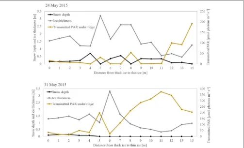
cored for biological analysis (Figure 1B), we encountered three ledges on top of each other with voids between them. The three ledges at the star sampling point (Figure 2), from top to bottom were 1.29, 0.88, and 1.69 m thick on 28 May, and 0.23, 0.80, and 0.55 m on 31 May. The decrease in thickness was probably a combination of melting and spatial variability. In general, across the ridge, from 24 to 31 May, both snow depth and sea-ice thickness decreased (Figure 4). The rubble macro-porosity of the unconsolidated submerged part of the ice, which represents the percentage of voids in between the ice ledges, was 25% on 24 May and decreased to 16% on 31 May. On 28 May, snow thickness was 0.13–0.22 m on the thick ice side (square) of the ridge, while it was 0.07–0.11 m on the refrozen lead side (star) (Figure 2).
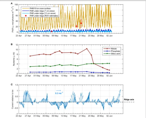
Incoming PAR averaged from 7, 18 and 20 May was 786±21 µmol photons m−2s−1(average and standard deviation). PAR
transmitted through the ridge varied between 0.1 and 8.5% of the incoming PAR. The average transmitted PAR below the ridge was 24±10µmol photons m−2s−1(n=334) (n is the number of
samples), i.e., about 3% of the average incoming PAR, based on ROV measurements at 0–5 m below the ridge. This was higher than light transmitted through the thicker ice (Average 0.37±
0.08µmol photons m−2s−1,n=44638) and lower than through
the thin refrozen lead (Average 114±69µmol photons m−2s−1, n=55) measured during the N-ICE2015 expedition (Taskjelle
et al., 2016; Kauko et al., 2017; Olsen et al., 2017). However, from the videos we observed that transmitted light was highly variable and patchy inside the ridge structure. Bright spots were observed inside the ridge in between the ledges (see Video in Supplementary Material).
Since light transmission measurements below ridged areas were scarce, we also attempted to model in a simplistic way thePARtransmitted through the ridge based on the snow and ice thickness and based on optical properties (cf. section Light Measurements and Calculations). ThePARtransmitted through the thick-ice side of the ridge was lower (average on 24 May: 9 µmol photons m−2 s−1; average on 31 May: 59µmol photons
m−2s−1) than through the thin-ice side (average on 24 May: 62
µmol photons m−2s−1; average 31 May: 274µmol photons m−2
s−1;Figure 4). This coincides with higher snow accumulation on
[image:7.595.48.551.372.678.2]the thick side of the ridge compared to the thin ice side. On 28 May, snow depth ranged between 0.07 and 0.11 m at the thin ice side of the ridge, so we calculated the theoretical minimum and maximum light transmitted through that specific spot from 23 April to 3 June to estimate temporal variability according to measured incoming irradiance (Figure 5A). The calculated transmittedPARat one spot, without taking into account changes in snow and ice light attenuation coefficients as the melt season progressed, was generally one order of magnitude lower than the measured PAR with the ROV, except on 7 May when they
FIGURE 5 |Overview of the conditions during Floe 3 with time series of(A)incoming Photosynthetically active radiation (PAR) measured above the ice (yellow) and calculated below the ridge for two snow thicknesses (dark blue: 0.07 m and light blue: 0.11 m) and the ice ledge thickness on 31 May. The red dots represent average and standard deviation of ROV measurements performed on 7, 18, and 20 May; note that PAR values above the ice (yellow) have been scaled down by a factor of 10 for clarity purposes;(B)Nutrient concentrations (nitrate, phosphate, and silicic acid) at 5 m depth below the ice;(C)Ocean current speed relative to the ice depicted by the arrows size and direction relative to the ridge axis at 23 m depth depicted in the y-axis (from vessel-mounted ADCP).
compared well (Figure 5A). The ROV measurements covered a wide area below the ridge and included lateral light sources since measuring depth was up to 5 m below the ridge (Katlein et al., 2016). Therefore, when comparing the measurements with the transmitted PAR calculated across the ridge we do encounter similar values, especially toward the thin ice side where the influence of the refrozen lead allowed more light to penetrate. The spatial variability of calculated light transmitted across the ridge (Figure 4) indicates that changes in snow depth and ice thickness were the major drivers of light-transmission variability.
Nutrient concentrations in the water column (at 5 m depth) between 28 April and 25 May were 8.4 ±0.8µM nitrate, 3.4
± 0.4µM silicic acid and 0.6 ± 0.1µM phosphate (average
and standard deviation) (Figure 5B). After the development
of a Phaeocystis-dominated under-ice bloom in the water
column (26 May−2 June) (Assmy et al., 2017), nitrate concentrations were reduced to 2.4± 1.2µM and phosphate to 0.4± 0.1µM, while silicic acid increased slightly to 4.1 ±
0.1µM (Figure 5B) as we drifted into more Atlantic-influenced waters.
Overall currents were weak, averaging 0.1 m s−1relative to the
ice, and came from various directions during the study period (23 April−5 June). However, over the period from 30 May to 5 June, current speeds larger than 0.2 m s−1were observed with a
mean relative current speed of 0.3 m s−1flowing in a north-east
part of the ridge facing the refrozen lead was on the lee side of the stronger currents (Figure 2).
Algal Communities in FYI Ridges
Dense accumulations of algae were observed by naked eye on the top and bottom of the ledges during the entire sampling period (10 May to 3 June;Figure 7and Video in Supplementary Material). When sampling these surfaces communities, a clear distinction became apparent between the bottom of the ledges and their vertical surfaces, and the top of submerged ledges. The bottom and the vertical wall communities were dominated by the pennate sea-ice diatoms Nitzschia frigida and Navicula
species, while the top community was dominated byShionodiscus
bioculatus(Figure 6A). Pennate diatoms of the genusNavicula
increased their dominance from 10 to 31 May. The fluffy algal layer that accumulated on the top of submerged ledges and was dominated byS. bioculatuscould be easily washed off by divers. A more diverse community was revealed in the ice cores taken from the ridge (Figure 6B). The three species that dominated the internal ice community on 31 May were F. cylindrus, N.
frigida,andPseudo-nitzschiasp. Three days later, on 3 June, the
percentage of dinoflagellate cysts increased from<10% to>25%. On that day, the most abundant diatoms werePseudo-nitzschia
[image:9.595.46.553.219.677.2]sp. andN. frigida(Figure 6B).
T A B L E 1 | C o n tin u e d S a mp le ID D a te (2 0 1 5 ) S a mp le ty p e M o s t a b u n d a n t a lg a l s p e c ie s Ic e th ic k n e s s s a mp le d C h l a P O C P O N B S i C :N mo la r N :S i mo la r Q u a n tu m y ie ld o f p h o to s y s te m II ( 8PSI I ) P ma x (r E T R ) In it ia l s lo p e ( α ) Ek U n it s (m) (mg m − 2) (mg m − 2) (mg m − 2) (mg m − 2) (– ) (– ) (– ) (– ) [mo l e -( mo l p h o to n ) − 1] [ µ mo l p h o to n s m − 2s − 1] R I1 9 3 1 M a y L e d g e 1 Fr ag ila rio ps is cy lin dr us . N itz sc hi a fri gi da 1 .2 9 2 7 .8 7 1 0 7 1 .0 1 4 3 .6 7 6 .7 8 .7 0 3 .7 4 – – – – R I2 0 3 1 M a y L e d g e 2 Fr ag ila rio ps is cy lin dr us . N itz sc hi a fri gi da 0 .8 8 1 9 .1 8 5 3 7 .5 7 8 .4 2 0 .6 8 .0 0 7 .6 3 0 .3 9 3 0 0 .0 4 7 5 0 R I2 1 3 1 M a y L e d g e 3 Fr ag ila rio ps is cy lin dr us . N itz sc hi a fri gi da 1 .6 9 2 6 .9 5 6 3 8 .8 9 2 .7 5 9 .5 8 .0 4 3 .1 2 – – – – R I2 2 3 Ju n e L e d g e 1 P se ud o-ni tz sc hi a sp . 0 .2 3 6 .7 8 2 3 0 .2 2 9 .1 9 .0 9 .2 3 6 .4 6 – – – – R I2 3 3 Ju n e L e d g e 2 P se ud o-ni tz sc hi a sp . a n d re st in g sp o re s 0 .8 0 1 1 .0 4 5 6 4 .3 7 5 .3 2 6 .8 8 .7 4 5 .6 0 – – – – R I2 4 3 Ju n e L e d g e 3 Fr ag ila rio ps is cy lin dr us 0 .5 5 8 .5 8 3 3 9 .7 5 0 .2 5 3 .9 7 .9 0 1 .8 6 – – – –
Samples taken at the ridge and the biogeochemical and photosynthetic parameters measured are summarized inTable 1. Chlaconcentrations in the slurp gun samples from the beginning of May ranged between 0.3 and 9.9 mg m−2. In late May and early
June, the volumetric Chlaconcentrations, from melting entire cores from the ledges, ranged between 13.8 and 29.4 mg m−3
(n=6) at the thin ice side, which correspond to an integrated Chlastock of 26–74 mg Chlam−2. The thick ice side had lower
Chlaconcentrations (4–11 mg m−3,n=2) which correspond
to 0.4–1.3 mg Chl a m−2 based on one bottom and one top
10-cm section (Table 1); therefore the biomass in the thick ice is probably underestimated. The integrated POC on the thin ice side of the ridge was 1,134–2,247 mg C m−2 (94–187 mmol
C m−2), the PON 154–314 mg N m−2(11–22 mmol N m−2), and
the biogenic silica 9–77 mg Si m−2(0.3–2.7 mmol Si m−2). The
C:Chlaweight ratio of the integrated biomass in the three ledges was 35.8±9.6, the C:N molar ratio of the organic material was 8.4
±0.5, and the N:Si molar ratio 4.7±2.1 (n=6) (Table 1). The maximum nutrient demand of the integrated ridge community on 31 May was 15.7 mmol N m−2 d−1 and 38.9 mmol Si m−2
d−1based on an estimated growth rate of 0.7 d−1(derived from
Chlameasurements on 31 May and 3 June) and the measured N:Chlaw:w ratio of 4.25 and the Si:Chlaratio of 2.11.
The photosynthetic acclimation of the diatoms to the prevailing light climate was assessed with photosynthetic parameters obtained from RLCs. The maximum dark-adapted quantum yield (ϕ) of the slurp gun and scrape samples was 0.40 ± 0.16 (n= 9) for Nitzschia-dominated bottoms of the ledge, and 0.42±0.11 (n=5) for theShionodiscus-dominated top part of the ledge (Table 1). Variability was very high (range: 0.19–0.61), but most samples were photosynthetically healthy with no evidence of chronic photoinhibition in the dark-adapted yield data. In addition, on-board observations of silica stain uptake samples revealed that theN. frigidabottom community and the S. bioculatus surface community were growing and taking up silicate at the time of sampling (Figures S3A–D). The photoacclimation parameter (Ek), calculated from
electron transport with the PhytoPAM, was higher but highly variable forNitzschia-dominated communities (421±295µmol photons m−2 s−1) and slightly lower with less variability for
Shionodiscus-dominated communities (266±86µmol photons
m−2s−1). No statistically significant differences were detected in
the light-response parameters between these two communities (ANCOVA test for comparison of regression lines;Sokal and Rohlf, 2012).
The sympagic amphipod Apherusa glacialis was the most dominant ice fauna species. Other amphipods present were
Themisto libellula, Gammarus wilkitzkii, Onisimus glacialis,
and Eusirus holmi. Some zooplankton species, such as the
copepodsOithona similis, Calanus glacialisand undetermined Harpacticoida were present, although in lower numbers (Table S2).
Snow-Ice Interface Properties
TABLE 2 |Compilation of biogeochemical parameters of the snow-infiltration communities (SI).
Sample ID Date (2015) Chla POC PON C:N molar Salinity Nitrite Nitrate Phosphate Silicic acid
Units (mg m−3) (mg m−3) (mg m−3) (–) (–) (µM) (µM) (µM) (µM)
SI1 09 June 110.85 3170.0 435.7 8.49 10.90 n.d. n.d. n.d. n.d.
SI1 09 June 135.46 3683.5 522.2 8.23 6.50 n.d. n.d. n.d. n.d.
SI1 10 June 362.46 15002.4 2102.1 8.33 18.00 0.13 1.09 1.90 1.85
SI1 13 June 111.50 6701.6 1078.1 7.25 17.70 0.20 2.21 4.91 4.74
SI2 15 June 14.93 4616.4 608.4 8.85 17.50 0.11 0.40 2.73 8.97
SI3 15 June 2.61 3870.6 414.1 10.91 15.30 0.15 1.03 1.92 5.84
SI4 17 June 1.62 907.8 99.1 10.69 13.80 0.07 1.06 0.29 1.01
SI5 17 June 38.11 5701.3 680.9 9.77 21.10 0.46 0.40 3.12 3.52
SI6 18 June 0.37 692.6 59.0 13.71 10.00 0.06 0.64 0.18 0.70
SI7 18 June 42.25 552.9 74.7 8.64 12.10 0.06 0.40 2.45 6.49
SI8 18 June 46.06 2663.3 317.5 9.79 10.80 0.13 1.48 3.62 11.58
By 18 June, the modal ice thickness decreased to 0.8 m due to a strong bottom melting event, while the snow thickness remained in the same range (Rösel et al., 2018). Penetrating swell caused a breakup of the icepack into scattered 100– 200 m pieces on the morning of 19 June. The snow depth at the first snow-ice interface sampled (0.7 m) was thicker than the mean snow depth of 0.32 ± 0.20 m on Floe 4 (Rösel et al., 2018). When the relation between ice thickness and snow thickness exceeded the hydrostatic equilibrium, the thick snow cover pushed the ice below sea level creating areas of negative freeboard. Based on drill hole measurements, 53% of the area of Floe 4 had negative freeboard (Rösel and King, 2017).
According to the snow pit performed on 13 June at SI1 (Figure S4), the top 0.3 m of the snow pack was hard wind slab of 0.5 mm grain size. The bottom 0.5 m consisted of refrozen melt layers of larger grain size (1.0 mm). The snow hardness decreased toward the bottom of the snow pack, close to the slush where the algae had accumulated (Figure S4). The temperature profile across the snow showed values around 0◦C in the upper 0.3 m and<0◦C in the lower 0.5 m (−0.1 to−1.2◦C). Compiling the information from the eight locations sampled (Figure 1C), the slush where the algae were found had thickness of 0.04– 0.2 m, temperature of −1.2 to −1.7◦C, and bulk salinity of 6.5 to 21.1 (practical salinity unit, henceforth unitless) (average 13.9 ± 4.3, n = 11; Table 2) in the melted slush depending on the amount of seawater that had percolated to the snow-ice interface. Snow infiltration communities were typically found in areas with thick snow (0.2–0.7 m), thin ice (0.4–0.9 m) in an advanced stage of melt, and were usually associated with cracks in the ice. Seawater percolated through the cracks in the ice toward the flooded snow-ice interface. Algae were found along the cracks and spreading ∼0.5 m to either side of the crack (Figures 7B,C).
The PAR transmittance through 0.2–0.4 m snow cover was 3–14% of the incoming irradiance based on measurements on 11 June at SI1 using a scalar PAR sensor. When using the average estimated snow light attenuation coefficient of 14.82 m−1for Floe
FIGURE 7 | (A)Underwater photograph of FYI ridge sampled on 31 May indicating the most abundant species of the bottom and top of the ledges. Microscopy images of the bottom of the first ledge shows the pennate diatom
Nitzschia frigida(RI19) and the top of the second ledge shows the centric diatomShionodiscus bioculatus(RI20).(B)Photo of the snow infiltration community SI1 found below 0.7 m of snow on 9 June 2015.(C)Photo of the snow-ice interface SI1 with a metric tape in cm scale to give an idea of its thickness.
FIGURE 8 |Relative composition of eight different snow infiltration communities based on cell abundance. Samples analyzed by light microscopy.
our calculations assume a downwelling light field. On an average sunny day (1,200µmol photons m−2s−1incoming PAR), algae
below 0.2 m of snow would receive 62µmol photons m−2 s−1
and 0.03 µmol photons m−2 s−1 below 0.7 m of snow. This
corresponds to 0.0025–5% transmitted PAR.
Algal Communities at the Snow-Ice
Interface
Snow infiltration communities were found at eight different spots on Floe 4 between 9 and 18 June (Figure 1C). The taxonomic composition of the snow-infiltration communities was very diverse and included both pelagic and ice-associated species. Besides a small percentage of flagellates, ciliates and dinoflagellates (sum of the three groups 3.4±2.8%), the snow infiltration communities were dominated by the haptophyte
P. pouchetii (51 ± 31%) and diatoms (42 ± 27%; Figure 8).
Phaeocystis pouchetii, which was the dominating species of the
under-ice phytoplankton bloom taking place at the same time, was present in the snow infiltration communities (8.3 × 10⁵
-8.7 ×10⁷ cells L−1) in similar concentrations as in the water
column (8.6×10⁵-9.9×10⁷cells L−1;Assmy et al., 2017). The
dominant pelagic diatoms present wereF. oceanica,C. gelidus,
Pseudo-nitzschiasp. and Thalassiosira spp.; and the main
ice-associated diatoms wereF. cylindrus, Naviculasp. andNitzschia
sp. (Figure 7). However, some species such asF. oceanicaandF.
cylindruscan be quite abundant in both sea ice and the water
column making the pelagic vs. ice-associated distinction difficult. In terms of diatoms, most snow-ice interface communities were dominated by a typical pelagic algal composition except for SI6 that had a more ice-algal composition (Figure 7). This sample had very low counts and a higher percentage of resting spores than all the others, indicating a senescent stage. Also, in many of the snow-ice interface communities, a high percentage of the
P. pouchetiicolonies observed were decaying and contained very
few cells (3–70% of the community was P. pouchetii cells in bad shape), indicating that this species infiltrated from the water column but was not performing optimally in its new habitat.
The Chlaconcentration in the slush collected at the snow-ice interface ranged three orders of magnitude: from 0.37 to 362 mg m−3(Average: 69±115 mg m−3,n=11;Table 2). The POC was
552–15,000 mg C m−3and the PON 59–2,102 mg N m−3(n=11)
FIGURE 9 |Rapid light curves from ridge (black circles) and snow infiltration (white circles) communities measured with PhytoPAM. The relative electron transfer rate (rETR) is plotted against photosynthetically active radiation (EPAR). Average and standard deviation for each light step are shown and theWebb et al. (1974)model was used to fit the average curve.
phosphate, had very high concentration. Nitrate ranged between 0.4 and 2.2µM, phosphate between 0.2 and 4.9µM, and silicic acid between 0.7 and 11.6µM (n= 11) (Table 2). The maximum nitrate demand of the snow-ice interface community was 17.8 mmol N m−2d−1at a growth rate of 0.62 d−1(calculated with
Chlavalues from 9 and 10 June in SI1) and a N:Chlaratio of 5.7. On-board observations of silica stain uptake samples revealed that the diatoms were growing and taking up silicic acid at the time of sampling (Figures S3E, F), while light microscopy analysis revealed a high percentage of decayingP. pouchetiicells. This variability in the physiological status of the algae at the snow-ice interface was reflected in the photosynthetic activity measurements performed with the PhytoPAM. The 8PSII, at SI1 during 5 days (9, 10, 11, 13, and 14 June), ranged between 0.22 and 0.46 (n= 5) indicating that only part of the snow-ice infiltration community was healthy. The low salinities at SI1 (6–18) could be responsible for the decayingP. pouchetii cells. The photoadaptation parameter (Ek) ranged between 156 and 453 µmol photons m−2 s−1. When comparing the snow-ice
interface community with the ridge communities, we found that ridge communities had significantly higher light saturation level (ANCOVA test for homogeneity of regression curves;Sokal and Rohlf, 2012), implying that these communities were acclimated to higher light intensities than the snow infiltration community (Figure 9).
DISCUSSION AND CONCLUSIONS
Contribution of FYI Ridges and Snow-Ice
Interfaces to Arctic Algal Biomass and
Sampling Challenges
Algal accumulations in complex structures such as ridges and in hidden layers at the snow-ice interface are understudied in
the Arctic Ocean and thus have not been accounted for in sea-ice algal biomass estimates. In this study, we have estimated the contribution of ridge and snow infiltration communities to the total ice algal biomass for the first time (Table 3) based on RadarSat-2 satellite scene ice-type classification (Figure S1),in situnegative freeboard measurements, and the measured Chla
in each sea-ice environment.
Ridges and rubble ice could contribute 36–96% of the total sea-ice biomass, assuming that all of this area would sustain the same amount of biomass as the thin ice side of the ridge we sampled (Table 3). In reality, the percent contribution was probably lower since not all ridges are FYI ridges close to a refrozen lead. Indeed, in our study region, only 2.8–7.4% were deformed edges next to open water or young ice (Table 3). If only this particular type of ridge would host algal biomass as we observed in the thin ice side of our study ridge (26–74 mg Chl
am−2) and the rest of the ridges and deformed areas would only
host as much biomass as we observed on thick ice side of the ridge (0.4–1.3 mg Chlam−2), their contribution would be 34–75% of
the total sea-ice biomass (Table 3). Nevertheless, compared to other sea-ice environments (FYI, new, and young ice), ridges and deformed ice areas, can account for most of the sea-ice related biomass. This is in agreement with large-scale under-ice ROV surveys that point toward ridges as relevant for algal biomass accumulation (Lange et al., 2017b). It is therefore critical that ridges are examined more closely and included in biomass and productivity estimates for Arctic sea ice.
Snow infiltration communities, which in the Antarctic can be responsible for most of the ice-associated production (Arrigo et al., 1997) and biomass (0.5–30 mg Chl a m−2; Arrigo and Thomas, 2004), seem to have a smaller contribution in the Arctic. Assuming a minimum thickness of the slush layer of 0.04 m, the integrated Chlawas 0.01–14 mg m−2. On a larger scale, if
all areas with negative freeboard would be inhabited by these communities, algal standing stocks on flooded sea ice could potentially reach 0.1–3.4 mg Chlam−2 and contribute 9–32%
to the total sea-ice integrated Chl a(Table 3). The minimum percent contribution of snow infiltration communities (9%) to total ice algal standing stocks was tenfold higher than the minimum contribution of ice algal biomass in level FYI and SYI (0.9%). Thus, including snow infiltration communities in sea-ice biomass and productivity estimates is relevant, especially during the late productive season when the ice starts melting and bottom sea-ice production decreases (Leu et al., 2015). However, these communities were usually only found along cracks in the ice and not in all flooded areas. Unfortunately, there is currently no way to quantify the percentage of the flooded area covered by cracks in the ice, so the estimate provided is just a potential maximum of the real contribution.
samples collected by divers, in otherwise inaccessible cavities and structures of the ridges, seem to be better suited for determining the dominant algal species concentrated at the surface of the submerged ledges compared to ice coring. The latter will likely result in the loss of loosely attached surface communities, such as the fluffy layer ofS. bioculatus, during core retrieval. Coring of the entire ridge on the other hand will provide information on the internal ice community structure and biomass. Thus, a combination of ice coring and slurp gun sampling or ice coring from below by divers would be the best approach to assess both qualitatively and quantitatively the algal community in ridges.
ROVs can be used to study the optical properties and derive algal biomass from light transmission. However, ROVs are likely to get entangled in complicated under-ice structures and therefore, measurements are usually taken several meters below the ridge (Lange et al., 2016), integrating light from a broad area under the ridge. Smaller ROVs with better maneuverability might be a solution to map the spatial variability in light penetration and algal biomass inside the ridge structure, but divers are needed to obtain measurements inside specific structures. In addition, specific modeling approaches need to be developed to describe the complex light regime inside the ridge structure, since simple 1D vertical models, like the one we used, fail to reproduce the observed complex light field inside the ridge.
The challenge in the case of snow infiltration communities is to detect them since they are covered by snow and therefore not readily visible from the surface, except at the edge of ice floes (von Quillfeldt et al., 2009). In addition, upscaling of the potential habitat suitable for snow infiltration communities requires a good knowledge of the percentage of the ice floe that has negative freeboard. In this study, we based our estimates on
in situobservations from several kilometer long transects with
EM31 (Rösel et al., 2016a), the snow probe (Rösel et al., 2016b), and drill holes (Rösel and King, 2017). Satellites cannot detect infiltration layers at the snow-ice interface (Ackley et al., 2008). Detecting potential zones of surface flooding is challenging due to the difficulties in differentiating wet melting snow from surface flooding (Onstott, 1992). It is therefore necessary to be either in person in the field or have autonomous instruments such as Ice Mass Balance buoys deployed on the ice to qualitatively observe rapid sea-ice melt events. However, knowing the potentially flooded area does not give any information on where the snow infiltration communities grow. Our observations indicate that they concentrate along cracks in the ice, and these are difficult to detect when covered with snow, and therefore, difficult to upscale. Despite the potential local importance of snow infiltration communities, their upscaling is challenging and this study is just a first attempt to estimate their contribution to ice-associated algal biomass that needs to be further refined.
The Role of Ridges and the Snow-Ice
Interface as Algal Safe Havens: Irradiance,
Nutrients, and Grazing Pressure
The high algal biomass encountered in ridges and at the snow-ice interface during the 2015 productive season in the high
Arctic indicates that these two environments provide shelter TA
and favorable conditions for algal accumulation and potentially growth.
Newly formed FYI ridges with complex ice structures offer plenty of cavities and surfaces for attachment and deposition (16– 25% voids). The complex structure of sea ice piled up in ridges creates an extensive habitat for sea-ice algae which exceeds other sea-ice related environment in terms of its total surface area, with the exception of Antarctic platelet ice. Indeed, other studies have reported higher macro-porosity values of 30–35% (Høyland, 2007; Strub-Klein and Sudom, 2012). In addition, the lee side of ridges provide algal communities protection from under-ice water currents, particularly for those algae that are loosely attached to ice surfaces such as the communities dominated
byS. bioculatus. Therefore, higher biomass concentrations are
expected on the lee side or hydrodynamic shadow of ridges. This effect has been suggested to explain accumulation of diatoms (Melnikov and Bondarchuk, 1987; Krembs et al., 2002), algal aggregates (Katlein et al., 2015b), as well as ice fauna (Hop and Pavlova, 2008; Kiko et al., 2017) in sheltered areas of ridges. Indeed, ridges are hot spots for accumulation of sea-ice fauna (Gradinger et al., 2010) since the organisms can graze on the abundant surface-attached sea-ice algae. For example,A. glacialis, which was the most abundant ice-associated amphipod in this study, has been shown to actively feed on ice algae, which can be a main contribution to its diet (Werner, 2000; Brown et al., 2017). The snow-ice interface on the contrary provides shelter from grazing since only small ciliates were observed grazing on the snow infiltration community (Figure 8). In addition, the low salinity in the slush (6–21) would reduce the grazing activity of potential grazers that could reach this layer. This lack of strong metazoan grazing pressure in the infiltration community environment could have favored the accumulation of algal biomass. Processes of physical concentration of algal biomass in the slush could also be responsible for the high accumulation of biomass. Since the highest algal biomass accumulations occurred within half a meter around cracks in the ice, we hypothesize that infiltrated communities concentrated in these areas, trapped in the porous snow-ice slush as water percolates to the rest of the floe.
The accumulation of snow on the side of ridges (Chapters 3 and 4 in Thomas, 2017) has likely led to the assumption that light transmission through ridges is very low. However, according to our observations, inside the complex ridge structure there are cavities that appear as bright areas inside the ridge. Bright areas were present especially in ridges associated with leads and thin ice (Figure 2and Videos in the Supplementary Material). Furthermore, cracks at the sides of ridges (Katlein et al., 2015a), as well as often snow-free portions of high points in a ridge due to wind erosion (Sturm and Massom, 2010) have been suggested to transmit more light than adjacent level thick ice (Lange et al., 2017a). In addition, the side with less snow and close to the thin ice received more light and could therefore support higher algal growth rates, assuming light limitation at the thick-ice side (Table 1).
Snow infiltration communities received more light (PAR transmittance 3–14%) than ridge algal communities (PAR transmittance 0.06–8.5%) according to in situ measurements
depending on the snow depth. This transmittance values were similar to those measured below ridges by an ROV in the Central Arctic (up to 5%) (Lange et al., 2017b), and lower than the PAR transmittance in the thin ice next to the ridge (5–40%) (Kauko et al., 2017). However, in situ measurements below the snow might be affected by lateral spreading of radiation and light scatter when removing part of the snow cover to introduce the sensor. CalculatedPARtransmittance at the snow-ice interface (0.0025–5%) is generally lower than at the ridges (0.12–71%, range from transects inFigure 4) especially at the thin ice side. In some cases, the snow-ice interface received one order of magnitude more light than the water column below thick ice (Olsen et al., 2017). This implies that the snow-ice interface, when flooded, might provide an advantage for infiltrated pelagic diatoms that were growing at low rates in the water column at that time (Assmy et al., 2017).
The other key factor for algal growth is nutrient availability. The algal communities growing on the surfaces of submerged ledges in ridges have direct access to the nutrients in the sea water (Figure 2), while the ones in the snow-ice interface are dependent on the nutrients availablea prioriin the snow-ice layer and those percolating upwards from the water column (Figure 3). The observed currents below the ice crossed the ridge from the thick-ice side to the thin-thick-ice side most of the time, especially toward the end of May, when stronger currents were observed (Figure S2). Before we drifted into the under-ice phytoplankton bloom (Assmy et al., 2017), the currents could have provided a constant flux of nutrients to the ridge surface-attached communities. Diatoms are able to store nutrients intracellularly without using them for growth immediately (Kamp et al., 2011; Fernández-Méndez et al., 2015). Based on our nutrient and current measurements, before 25 May (pre-bloom) one centimeter water layer moving below the ice provided 1.56×10³-7.78×10³mmol
N m−2d−1and 5.18×10³-2.59×10³mmol Si m−2d−1, which
is two orders of magnitude more than the calculated nutrient demand for these communities (15.7 mmol N m−2 d−1 and
38.9 mmol Si m−2 d−1) using the method explained inCota et al. (1987)and our own measured ratios and growth rates. This calculation suggests that the algae fixed to the ridge surfaces are flushed with enough nutrients to support their growth demands. Nevertheless, the currents and nutrient uptake dynamics inside the ridge and at the ice-water interface would need to be resolved better in order to assess the reality of the nutrient supply and limitations. The high C:N ratio (8.4±0.5,n=6) of the integrated biomass in the entire ledges might be due to the higher fraction of dead cells and/or detritus inside the ice as compared to the surface layers.
precipitation (Nomura et al., 2010). A re-supply of nutrients can eventually come from the infiltrated surrounding seawater. At the time when the snow-ice infiltration communities were observed, nitrate concentrations in the water column were relatively low due to uptake by the under-iceP. pouchetiibloom (Figure 4B). However, if the ice had been previously flooded, nutrients from a different water mass could have been trapped in this layer. During the winter months of the N-ICE expedition, snow-ice formation was observed in February-March in ice floes of the same area and similar conditions (Granskog et al., 2017; Merkouriadi et al., 2017). Nutrient concentrations in the snow/slush sampled in March 2015 reached values up to 17µM nitrate, 1µM phosphate and 4µM silicate. This amount of nitrate could yield 42 mg Chla
m−3, which is one order of magnitude less than the maximum
Chl aconcentrations observed in the slush layer (362 mg Chl
am−3 SI1,Table 2). This indicates that the winter pre-formed
nutrients are insufficient to explain the high biomass observed at the snow-ice interface.
In addition, the fact that we found several species of pelagic diatoms growing in the snow-ice interface points toward a flooding of the ice and establishment of the infiltration community in a different water mass with a more diatom-dominated phytoplankton community than the one we observed. Backtracking of Floe 4 (Olsen et al., 2017, Figure 1) indicates that the floe was closer to the shelf break some weeks earlier and these waters might have hosted a different phytoplankton community than the P. pouchetii dominated community observed on the Yermak Plateau. Indeed, the presence of abundant pelagic diatoms in surface waters on 8 June (Assmy et al., 2017) could explain the presence of pelagic diatoms in the snow-ice interface. On the other hand, the haptophyte
P. pouchetii, despite being present in high cell abundance,
was not performing well, indicated by the high amount of disintegrated cells and colonies observed under the microscope (Figure 8). These dead cells might be the reason for the high C:N ratio.
Distinct Algal Communities Occupy
Different Ridge Surfaces
One interesting aspect of understudied ridge environments is that they seem to favor specific algal communities. Inside ridges, two clearly distinct communities were observed at the bottom and at the top of the submerged ledges (Figure 7A). A mixture of sea-ice pennate diatoms dominated byN. frigidaand
Navicula species at the bottom of the ledges is in accordance
with previous observations of FYI and MYI, in which these species are dominating the bottom of the sea ice (Syvertsen, 1991; Melnikov et al., 2002). Sea-ice pennate diatoms excrete extracellular polymeric substances that enable them to attach inside brine channels at the under-side of the ice (Krembs et al., 2000, 2011; Bowman, 2013). On the contrary, the centric diatom
S. bioculatusseems to have a clear advantage for colonizing the
top of ledges (von Quillfeldt et al., 2009) as a fluffy algal layer since this species is not able to actively attach to the ice. This fluffy layer can be easily washed off by strong currents which agrees with previous observations of Arctic ridge communities
(Hegseth, 1992; Ambrose et al., 2005). Furthermore, their presence supports the protective role of interior ridge cavities from currents (Figure 2).
The difference in the photoacclimation parameter (Ek)
between the Nitzschia (421 µmol photons m−2 s−1 on
average) and the Shionodiscus-dominated communities (266 µmol photons m−2s−1on average) might indicate that different
parts of the submerged ledges receive on average different light intensities that favor different species that are able to acclimate to those light conditions. For example, S. bioculatus is more light sensitive and better shade adapted since it usually performs poorly under high light environments such as melt ponds (Assmy et al., 2013). Small-scale light measurements inside ridges and a spatially resolved light transmission model for complex under-ice structures are needed to further confirm this hypothesis.
Diatoms vs.
Phaeocystis
at the Snow-Ice
Interface
The snow-ice interface had no distinct biotopes within the slush layer. Nevertheless it is interesting to compare the species that accumulated in the infiltration layer with the ones in the water column, which in this study was the source of the snow infiltration community. In the literature there are examples of snow-ice interface layers dominated byPhaeocystis(McMinn and Hegseth, 2004), by diatoms (Buck et al., 1998), or by a mixture of both (Kristiansen et al., 1998). During our study, we encountered five snow infiltration communities dominated by P. pouchetii
(SI1, SI2, SI5, SI7, and SI8), and three dominated by diatoms (SI3, SI4, and SI6), although both groups were present in all of them. Differences inPhaeocystisvs. diatom dominance could reflect differences in phytoplankton composition in the source waters when infiltration occurred through the cracks in the ice or the time since flooding occurred at a particular site, the latter on the scale of community succession.Phaeocystis pouchetiiwas the most abundant species based on cell numbers in the water column at the time of sampling (Assmy et al., 2017), which is consistent with its presence in the infiltration community. This species is supposed to be very plastic since it can adapt its photosynthetic efficiency to the rapidly changing light regime (Palmisano et al., 1986; Cota et al., 1994; McMinn and Hegseth, 2004). However, during a side experiment, in which we removed the snow on top of SI1 and sampled it 24 h later, we could observe a decrease in the healthy cell numbers ofPhaeocystis and an increase in poor-quality cell numbers, with no significant change in the diatom composition (Figure S5). This indicates thatP.
pouchetiicould not deal with the rapid increase in irradiance and
that diatom frustules are more resistant to decay. The average Ek
of SI1 was 331±125µmol photons m−2 s−1 (n=5) and the
measured Ed(PAR) below 0.2–0.7 m of snow ranged between 1 and 162µmol photons m−2s−1. The difference between E
kand
Edindicates that the cells are adapted to a higher light intensity
Assmy et al., 2017), as well as the low salinities at the snow-ice interface (6.5–21), might have negatively affected part of the
P. pouchetiipopulation, while not having as deleterious impact
on the diatom portion of the community due to their rigid silica frustules. Similar findings have been observed in ice melt processing studies with respect to flagellate versus diatom species (Buck et al., 1998; Garrison et al., 2003). Pelagic diatoms such as
F. oceanica,C. gelidus, andPseudo-nitzschiasp. which were not
abundant in the water column at the time of sampling but might have infiltrated previously, managed to rapidly accumulate in the snow-ice interface (Figure 8and Figure S3).
Future Predictions and Implications
With the ongoing changes in the Arctic icescape due to anthropogenic climate change, a shift in community composition and productivity of sea-ice algae is expected (Dupont, 2012; Fernández-Méndez et al., 2015; Hardge et al., 2016; Olsen et al., 2017). During May-June 2015, the percentage of ridge and deformed ice cover was very high (46–51%), in agreement with recent airborne surveys indicating that ridged ice can make up a substantial fraction of the pack ice (Haas et al., 2010). For example, in Fram Strait from 1990 to 2011 ridges contributed 66% of the mean thickness of sea ice (Hansen et al., 2014). In the coming decades, as the ice gets thinner and more dynamic due to increased temperatures and wind (Spreen et al., 2011; Renner et al., 2014), an increase in FYI pressure ridge formation is expected (Wadhams and Toberg, 2012). As we have shown in this study, FYI ridges close to refrozen leads can host high biomass of healthy algal communities and could therefore play an important role in the Arctic icescape’s future productivity. We encourage future studies to focus on pressure ridges despite the sampling challenges, since they are an important and under-quantified part of the Arctic icescape.
The mean snow thickness observed on FYI on Floe 4 was 0.32± 0.20 m (Rösel et al., 2018), which is in the same range given in the Warren-Climatology based on observations from snow on thick MYI (snow of 0.33 m;Warren et al., 1999). Sea-ice and snow thicknesses have changed toward a thinner, FYI-dominated ice cover that had less time to collect snow than older ice (Gallet et al., 2017; Merkouriadi et al., 2017). The combination of thin and rapidly melting sea ice and a relatively thick snow cover, led to negative freeboard and flooding of approximately half of Floe 4. This situation might become more frequent in the future, as sea-ice thickness continues to decrease (Maslanik et al., 2007; Stroeve et al., 2012), while precipitation falling on sea ice has been predicted to increase north of Greenland and in the Eurasian basin of the high Arctic where the remaining ice will reside (Bintanja and Selten, 2014). In addition, in the Atlantic sector, the influence of an increasingly warm Atlantic water inflow will contribute to faster ice melt from below (Polyakov et al., 2017). Thus, the contribution of snow to sea-ice mass balance could increase (Granskog et al., 2017), with flooding events in early spring (Granskog et al., 2017; Provost et al., 2017). These conditions favor the accumulation of algae at the snow-ice interface. These snow-infiltration communities have been frequently observed in the Antarctic, where the ratio of snow-to-sea ice thickness is high. We hypothesize that
this “Antarctification” of the Arctic icescape will lead to more frequent accumulation of sea-ice algae at the snow-ice interface, especially in the Atlantic sector, and that snow infiltration communities might play a similarly important role in sea-ice related productivity in the future Arctic, as in the Antarctic (Arrigo et al., 1997).
The consequences of more algae accumulating in these two environments are still unknown, but we can hypothesize that ridges will become hot spots of biomass that will fuel the ice-associated food chain, since they will be accessible for grazers (Gradinger et al., 2010) and their carbon will be transferred to upper trophic levels (Falk-Petersen et al., 2009). On the contrary, snow infiltration communities will remain largely inaccessible for larger grazers during the productive season, although some grazers have been observed at the ice surface in Antarctic sea ice (Schnack-Schiel et al., 2001), and will likely sink when the ice melts, strengthening the sympagic-benthic coupling (Søreide et al., 2013) if they are not being decomposed and remineralized by bacteria. Moreover, the different algal species accumulating in these environments will influence how much carbon is exported to the seafloor, given that diatoms are more efficient carbon exporters than P. pouchetii (Reigstad and Wassmann, 2007). In terms of timing, while snow infiltration communities seem to appear only at the end of the productive season linked to ice melt, ridge communities are likely important year-round but particularly during the summer melt season when most ice algal biomass is lost from level sea ice. Thus, pressure ridges might act as refuges for the ice-associated flora and fauna during times of rapid melt and as an algal seed bank for newly formed ice.
The key points of this study are:
- Ridge algal communities can account for most of the sea-ice biomass when compared with other sea-sea-ice environments, while the snow infiltration communities are difficult to upscale since they occur below thick snow along cracks, but they are locally important for sea-ice biomass estimates at the end of the productive season.
- Ridges are a favorable environment for algal growth because they provide extensive surfaces for attachment, shelter from strong currents, light conduits and a sufficient nutrient supply. - Snow ice interfaces present high accumulations of algal biomass probably due to physical accumulation, higher irradiance than below the ice and shelter from grazers. - Ridges host distinct algal communities with different light
acclimation parameters and attachment strategies. Pennate sea-ice diatoms are found in the bottom part of the ledges, whileS. bioculatusforms a fluffy layer on the top part of the ledges.
- Infiltration communities were dominated by the haptophyte
P. pouchetii and pelagic chain-forming diatoms which were
performing better thanP. pouchetii.