Department of Physical Sciences
A long-term single-pulse study of the
Vela pulsar
Jim Palfreyman M.Sc.
Version 1.05
2018-10-31
MJD 58422.1
Supervisors:
Prof. John Dickey
Prof. Simon Ellingsen
Dr Aidan Hotan
Declaration of Originality
This thesis contains no material which has been accepted for a degree or diploma by the
University or any other institution, except by way of background information and duly
acknowledged in the thesis, and to the best of my knowledge and belief no material
previously published or written by another person, except where due acknowledgement
is made in the text of the thesis, nor does the thesis contain any material that infringes
copyright.
Signed:
Dedication
This work is dedicated to Stephen Atkinson (MJD 37693.2 to 58313.4). Technically
the oldest of my oldest friends.
In my teenage years, and being two years his junior, I followed in his footsteps through
high school, college, and then completed a Computer Science degree. This opened my
eyes to the world of science and commenced my academic career. I ended up adding a
mathematics degree to my B.Sc., then I completed Honours. Thirty years passed and I
lost contact with Stephen until we re-connected online. After completing my Masters
in Astrophysics and during this Ph.D. he was very supportive and the first to comment
upon me lecturing in mathematics and also being published in Nature.
My hatred of European wasps was only equalled by Stephen.
His untimely death occurred as this work was been finalised and it was particularly
devastating for me.
Authority of Access
The publishers of the two papers comprising Sections 6.1 to 6.4 on pages 133–142 and
Appendix C hold the copyright for that content, and access to the material should be
sought from the respective journal. Chapter 8 is an extended coverage of Appendix C,
but the content is quite different. This and the remaining non-published content of
the thesis may be made available for loan and limited copying and communication in
accordance with the Copyright Act 1968.
Signed:
Statement of Co-Authorship
The following people contributed to the publication of work undertaken as part of this
thesis:
Candidate
Palfreyman, J. L.
University of Tasmania
Co-Author 1
Dickey, J. M.
University of Tasmania
Co-Author 2
Ellingsen, S. P.
University of Tasmania
Co-Author 3
Hotan, A. W.
CSIRO Astronomy & Space Science
Co-Author 4
Jones, I. R.
University of Tasmania
Co-Author 5
van Straten, W
Auckland University of Technology
Sections 6.1-6.4
:
Temporal evolution of the Vela pulsar’s pulse profile
Candidate (85%), Co-Author 1, 2, 3, and 4 (15%)
Candidate was the primary author and Co-Authors 1, 2, 3, and 4 contributed to the
idea, its formalisation, development and refinement. Writing was done primarily by
the Candidate. Feedback and editing for the purposes of publication was provided by
the Co-Authors 1, 2, 3 and 4.
Appendix C
:
Alteration of the magnetosphere of the Vela pulsar during a glitch
Candidate (85%), Co-Author 1, 2, 3, and 5 (15%)
Candidate was the primary author and Co-Authors 1, 2, 3, and 5 contributed to the
idea, its formalisation, development and refinement. Writing was done primarily by the
Candidate. Polarisation calibration was done by Co-Author 5. Feedback and editing
for the purposes of publication was provided by the Co-Authors 1, 2, 3 and 5.
We the undersigned agree with the above stated “proportion of work undertaken” for
each of the above published peer-reviewed manuscripts contributing to this thesis:
Signed:
Signed:
Date:
31-Oct-2018
Date:
31-Oct-2018
Prof. John Dickey
Prof. Mark Hunt
Primary Supervisor
Head of School
School of Natural Sciences
School of Natural Sciences
“I’m looking at a stellar crematorium, staring
down the throat of a spinning dead star with a
1 pixel movie camera trying to figure out what
the hell happened.”
Abstract
Acknowledgements
I have many people to thank over the duration of this work. The data-gathering was
probably the most annoying aspect, especially as the glitch approached. For this I
would like to mainly thank Brett Reid and Eric Baynes for keeping the 26 m telescope
up and running. As well as providing day and night support, they also cut me some
slack when the Y-drive was leaking oil, solved the burned-out hydraulics motor issue
(multiple times), fixed the capacitors in the main drives (multiple times), and kept the
L-band receiver cooled (multiple times).
Special mention goes to Bev Bedson at Ceduna who kept the 30 m telescope running
through many issues. This involved driving out at odd hours and this was no doubt
extremely tiresome at times.
I’d like to thank all the other observers for putting up with my persistence as the
glitch approached - especially Jamie McCallum who also provided much patience and
assistance.
The Dean’s Summer Students for 2016/17, Nicholas Bochenek and Wesley Kean Tai,
provided valuable assistance in the tedious “eyeballing” of many thousands of pulsar
plots for the removal of RFI and tracking down
nulls
. Job Carr-Turbitt also found a
lovely sequence of consecutive bright pulses.
I’d like to thank Ogilvie High School student Scarlett Marston for asking such a
fantas-tic question at one of my school visits when I was explaining how glitches work.
There were also numerous inter-departmental and tea-room chats where problems were
solved and new ideas seemed to just pop out of nowhere. Mentions go to Dr Kym Hill,
David Hughes, Melissa Humphries, and also Emeritus Professor Peter McCulloch for
providing me with historical data to analyse. A special mention goes to Karen Bradford
who provided much support with regard to the machinations of the bureaucratic entity
that is a University.
Internet resources, when carefully selected, can be excellent and the folks on the
time-nuts
and the Facebook
astrostatistics
forums have also been invaluable. A special
mention goes to
time-nuts
administrator Tom Van Baak.
Supervision is an incredibly important part of a Ph.D and my main supervisors
Pro-fessor John Dickey and ProPro-fessor Simon Ellingsen gave me the support, and especially
the freedom, to explore the aspects of this work that I needed.
question I had. I would also like to thank Dr Willem van Straten for his insights with
regard to the pulsar magnetosphere and neutron star cores.
I would also like to officially acknowledge the Australian Government Research Training
Program Scholarship which helped fund this research and the Tasmanian Partnership
for Advanced Computing (TPAC) at the University of Tasmania, with funding from
the Australian Government through its NCRIS and RDSI programs for the use of the
2.3 PB storage facility, without which this project would not have been possible.
A penultimate acknowledgement goes to my mum, Jennie Clarke, and my aunt, Wendy
Weight, who proof-read this thesis from a non-scientific perspective.
Finally, and most importantly, I’d like to thank my partner Zonia Bell for suffering
through the four years of a hard-slog that is a Ph.D.
Contents
List of Figures
v
List of Tables
xi
1
Thesis overview
1
1.1
Notes on style . . . .
2
2
Introduction
3
2.1
Formation of pulsars . . . .
3
2.2
Emission . . . .
4
2.2.1
Drifting, nulling, mode changing, and switching . . . .
9
2.2.2
Bright and giant pulses . . . .
11
2.3
Rotation and age . . . .
13
2.3.1
Characteristic age . . . .
13
2.3.2
Energy loss . . . .
16
2.4
Interstellar medium . . . .
18
2.5
Arrival times
. . . .
19
2.5.1
Solar system barycentre . . . .
19
2.5.2
Timing noise
. . . .
20
2.5.2.1
Polynomial fits and timing artefacts
. . . .
20
2.6
Fast Radio Bursts . . . .
25
2.7
Glitch theory . . . .
25
3
Pulsars of interest
31
3.1
The Vela Pulsar - J0835−4510 . . . .
31
3.1.1
Discovery . . . .
31
3.1.2
Glitches . . . .
33
3.1.3
Pulse flux density . . . .
33
3.1.4
Consecutive bright pulses
. . . .
36
3.2
J1644−4559 . . . .
36
3.3
J0437−4715 . . . .
38
3.4
The Crab Pulsar - J0534+2200
. . . .
40
ii
CONTENTS
4
Instrumentation and software
43
4.1
Mount Pleasant . . . .
43
4.1.1
Calibration
. . . .
45
4.2
Ceduna
. . . .
49
4.3
Sampling . . . .
51
4.4
Software processing . . . .
51
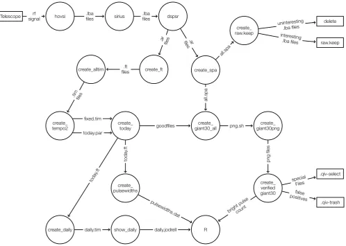
4.4.1
Data flow . . . .
51
4.4.2
Processing hardware . . . .
52
4.4.3
RDSI
petabyte disk storage . . . .
52
4.4.4
DSPSR
. . . .
52
4.4.5
TEMPO2
. . . .
57
4.4.6
PSRCHIVE
. . . .
57
4.4.7
Real time glitch detection . . . .
58
4.5
Radio frequency interference . . . .
58
4.5.1
Out-of-band RFI . . . .
59
4.5.2
4G mobile tower
. . . .
59
4.5.3
Lightning . . . .
59
4.5.4
Local transmission towers . . . .
66
4.5.5
Local mobile phones . . . .
66
4.5.6
Sparking terminal block . . . .
67
4.5.7
Aircraft . . . .
67
4.5.8
Unknown
. . . .
67
4.6
Statistical tools . . . .
69
4.6.1
R . . . .
69
4.6.2
Lomb-Scargle periodogram . . . .
69
5
Bright and giant pulses
81
5.1
Mount Pleasant observations . . . .
81
5.1.1
Integrated pulse profile flux density variations . . . .
81
5.1.2
Individual pulse flux density variations . . . .
83
5.1.3
Genuine giant pulses . . . .
85
5.1.4
Consecutive bright pulses
. . . .
89
5.1.5
Bright pulse from J1644−4559 . . . 100
5.1.6
Giant pulses from J0534+2200 . . . 100
5.1.7
Bright pulses leading the main pulse on Vela . . . 105
5.2
Vela pulse profile components by frequency . . . 108
5.2.1
Giant pulses as a component . . . 110
5.2.2
Profile edges . . . 111
5.2.3
J0437−4715 . . . 112
CONTENTS
iii
5.3.1
Same frequency . . . 128
5.3.2
Different frequency . . . 129
6
Temporal evolution of the pulse profile
133
6.1
Introduction . . . 133
6.2
Observations and data reduction . . . 134
6.3
Pulse shape changes
. . . 135
6.4
Conclusion . . . 142
7
Postscript with updated data
143
7.1
Micro-glitches . . . 150
7.1.1
Real or artefact? . . . 150
7.1.2
Linking micro-glitches to pulse width . . . 151
7.2
Morphology of pulse shape . . . 152
8
The glitch of 2016
155
8.1
Summary
. . . 155
8.2
Mount Pleasant results . . . 157
8.2.1
Fitting for the glitch . . . 157
8.2.2
A null . . . 159
8.2.3
Change in mean and variance . . . 161
8.2.4
Significance of RFI on timing and flux density . . . 161
8.2.5
Probabilities . . . 191
8.2.5.1
Probability of observing a null . . . 191
8.2.5.2
Probability of change in mean and variance . . . 192
8.2.6
The accurate glitch epoch . . . 194
8.2.7
Long-term changes in flux density . . . 194
8.2.7.1
Peak flux density changes . . . 195
8.2.7.2
Mean flux density changes . . . 195
8.2.7.3
Binning of data . . . 199
8.2.8
Detail of pulses surrounding the null . . . 199
8.2.8.1
Waterfall diagram of glitch
. . . 206
8.2.9
Rotational changes . . . 206
8.2.10 Combining flux density and rotation
. . . 213
8.3
Ceduna results
. . . 217
8.4
Discussion . . . 228
8.4.1
Solidifying superfluid? . . . 229
8.4.2
Ruling out a possible cause for FRBs . . . 229
8.5
Glitch vs micro-glitch . . . 229
iv
CONTENTS
8.7
Prediction . . . 232
8.7.1
History . . . 232
8.7.2
Cycling of ˙
ν
. . . 236
8.7.3
Prediction of ¨
ν
. . . 240
8.7.4
Cumulative glitch frequency changes . . . 240
8.7.5
Glitch magnitudes
. . . 243
8.8
Prediction results . . . 244
9
Conclusion
247
9.1
Summary
. . . 247
9.2
Further study . . . 248
Bibliography
251
Appendices
261
A Scripts, commands, and daily flow
263
A.1 Recording and glitch detection . . . 263
A.2 Copying . . . 264
A.3 Daily processing . . . 264
A.4 Analysis . . . 264
A.5 Calibration
. . . 264
A.6 Commands and tools . . . 265
B Data recording notes and summary
273
C Nature paper
311
List of Figures
2.1
Curvature radiation . . . .
6
2.2
Profiles of type Single (S)
. . . .
7
2.3
Profiles of type D, M, and T . . . .
9
2.4
Proposed spiral emission . . . .
10
2.5
Drifting sub-pulses from J0946+0951 . . . .
12
2.6
P
- ˙
P
diagram
. . . .
14
2.7
Characteristic age vs braking index of Vela . . . .
17
2.8
Fitting polynomials to
y
=
e
x
. . . .
23
2.9
Fitting polynomials to
y
= 100 sin(
x
) . . . .
24
2.10 Fitting polynomials to
y
= 100 sin(
x
) with a simulated micro-glitch
. .
25
2.11 Vortices in superfluid He II . . . .
26
2.12 Vortices in superfluid . . . .
27
2.13 Neutron star interior . . . .
28
2.14 Angular velocities of core vs pulsar . . . .
29
3.1
Optical images of the Vela pulsar . . . .
34
3.2
Chandra X-Ray image of the Vela Pulsar . . . .
35
4.1
Mt Pleasant receiver, mixing, digitisation, and recording chain . . . . .
45
4.2
Noise diodes . . . .
47
4.3
Software data flow diagram
. . . .
53
4.4
Processing times versus number of simultaneous processes
. . . .
55
4.5
Processing throughput versus number of simultaneous processes . . . .
56
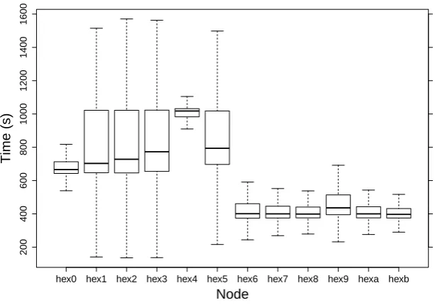
4.6
Processing times by node over 4 years . . . .
56
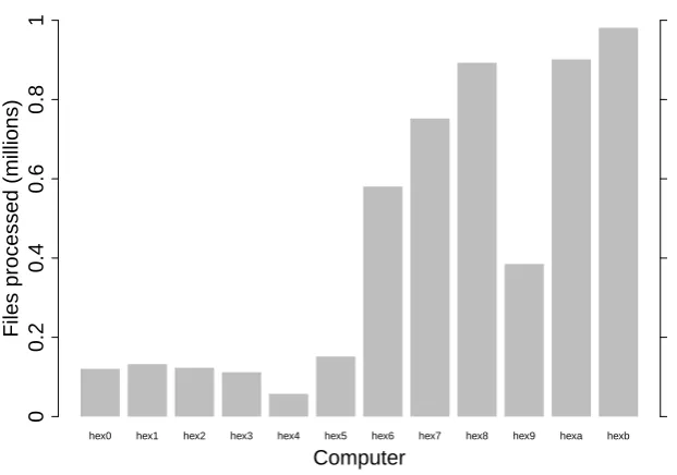
4.7
Processing throughput by node over 4 years . . . .
57
4.8
Telstra interfering transmitter beaming pattern
. . . .
60
4.9
A lightning strike that occurred
≈
10 km away . . . .
61
4.10 Lightning strike, pulse prior . . . .
62
4.11 Lightning strike, down stroke
. . . .
62
4.12 Lightning strike, return stroke . . . .
63
4.13 Lightning strike, final remains . . . .
63
4.14 Lightning strike, afterwards . . . .
64
4.15 Lightning strike, return stroke, zoomed-in
. . . .
64
vi
LIST OF FIGURES
4.16 Lightning strike, return stroke, extra high resolution . . . .
65
4.17 Flux levels for an entire observation . . . .
66
4.18 Spark RFI caused by a faulty terminal block . . . .
68
4.19 Lomb-Scargle periodograms of sinusoidal waves with multiple periods .
72
4.20 Lomb-Scargle periodograms with uniform noise 5-10 . . . .
73
4.21 Lomb-Scargle periodograms with uniform noise 20-30 . . . .
74
4.22 Lomb-Scargle periodograms with Gaussian noise
σ
=2.5-5 . . . .
75
4.23 Lomb-Scargle periodograms with Gaussian noise
σ
=10-15 . . . .
76
4.24 Sinusoidal signals with Gaussian noise and missing data points . . . . .
78
4.25 Lomb-Scargle periodogram of sinusoidal signals, Gaussian noise and
missing data points . . . .
79
4.26 Lomb-Scargle periodogram computation times . . . .
80
5.1
Average daily peak flux density for Vela and J1644−4559 . . . .
82
5.2
Lomb-Scargle periodogram of average daily peak flux density for Vela .
82
5.3
Histograms of pulse flux density . . . .
86
5.4
Brightest pulse, 8192 timing bins . . . .
87
5.5
Brightest pulse, 16384 timing bins . . . .
88
5.6
Brightest pulse, 32768 timing bins . . . .
88
5.7
Brightest pulse, 65536 timing bins . . . .
89
5.8
Brightest pulse, 1048576 timing bins
. . . .
90
5.9
Frequency vs Phase of the brightest pulse . . . .
91
5.10 Brightest pulse arrival in real time. Frame 1 of 8 . . . .
92
5.11 Brightest pulse arrival in real time. Frame 2 of 8 . . . .
92
5.12 Brightest pulse arrival in real time. Frame 3 of 8 . . . .
93
5.13 Brightest pulse arrival in real time. Frame 4 of 8 . . . .
93
5.14 Brightest pulse arrival in real time. Frame 5 of 8 . . . .
94
5.15 Brightest pulse arrival in real time. Frame 6 of 8 . . . .
94
5.16 Brightest pulse arrival in real time. Frame 7 of 8 . . . .
95
5.17 Brightest pulse arrival in real time. Frame 8 of 8 . . . .
95
5.18 Brightest 6 consecutive pulses discovered . . . .
96
5.19 Drifting sub-pulses on the Vela pulsar . . . .
96
5.20 Simultaneous drifting sub-pulse in opposite directions . . . .
97
5.21 “Impossible” drifting sub-pulse
. . . .
98
5.22 Simple graphic of core emission . . . .
98
5.23 Pulse 1/2 consecutive bright pulses . . . .
99
5.24 Pulse 2/2 consecutive bright pulses . . . .
99
5.25 A bright pulse from J1644−4559 . . . 101
5.26 The integrated pulse from J1644−4559 . . . 101
LIST OF FIGURES
vii
5.28 Integrated pulse over
≈
8 h from J0534+2200 at 1376 MHz . . . 103
5.29 The main pulse from J0534+2200 at 1376 MHz
. . . 103
5.30 The interpulse from J0534+2200 at 1376 MHz . . . 104
5.31 Giant pulse from J0534+2200 . . . 104
5.32 Peak flux density versus phase for Vela . . . 105
5.33 Peak flux density versus phase for J0534+2200 (main pulse) . . . 106
5.34 Peak flux density versus phase for J0534+2200 (main pulse, zoomed-in) 107
5.35 Peak flux density versus phase for J0534+2200 (interpulse) . . . 107
5.36 Peak flux density versus phase for J0534+2200 (interpulse, zoomed-in)
108
5.37 Gaussian components of pulse profile at 1376 MHz
. . . 113
5.38 Gaussian components of pulse profile at 2230 MHz
. . . 114
5.39 Gaussian components of pulse profile at 4800 MHz
. . . 115
5.40 Gaussian components of pulse profile at 6658 MHz
. . . 116
5.41 Gaussian components of pulse profile at 8425 MHz
. . . 117
5.42 Gaussian components of pulse profile at 12200 MHz . . . 118
5.43 Gaussian components of pulse profile at 22214 MHz . . . 119
5.44 Changes in component profiles over frequency . . . 120
5.45 Spectral index of component profiles
. . . 121
5.46 Gaussian components of pulse profile for brightest pulse . . . 122
5.47 Start and end of 1376 MHz integrated profile . . . 123
5.48 J0437−4715 profile at 1376 MHz
. . . 124
5.49 J0437−4715 profile at 4800 MHz
. . . 125
5.50 J0437−4715 profile at 6658 MHz
. . . 126
5.51 J0437−4715 profile at 8425 MHz
. . . 127
5.52 Spectral index of J0437−4715 . . . 128
5.53 Bright pulses at Mt Pleasant and Ceduna - same frequency . . . 129
5.54 Bright pulse at Mt Pleasant and Ceduna - different frequency
. . . 130
5.55 Giant pulse at Mt Pleasant at 1376 MHz . . . 131
5.56 Giant pulse at Mt Pleasant at 4815 MHz . . . 131
6.1
Pulse width, timing residuals, and bright pulse rate . . . 136
6.2
∆
ν/ν
= 75
.
6
×
10
−
9
magnitude micro-glitch at MJD=57143±3 . . . 137
6.3
∆
ν/ν
= 0
.
4
×
10
−
9
magnitude micro-glitch at MJD=56922±3
. . . 138
6.4
Lomb-Scargle periodogram of pulse width
. . . 139
6.5
Correlation of pulse width at 10% to 50% of the peak . . . 139
6.6
Angles of emission
. . . 140
6.7
Palfreyman vs Durant period comparison . . . 140
6.8
Integrated pulse profile - 750000 pulses . . . 141
viii
LIST OF FIGURES
7.2
10% pulse profile width of Vela
. . . 144
7.3
Bright pulse activity . . . 145
7.4
Correlation of 50% and 10% pulse profile width of Vela . . . 146
7.5
Lomb-Scargle periodogram of 50% profile width of Vela . . . 146
7.6
Pulse profile width of J1644−4559 . . . 148
7.7
Lomb-Scargle periodogram of profile width of J1644−4559 . . . 148
7.8
Vela pulse profile width at the 50% level during a single day . . . 149
7.9
Effect of timing residuals after changing pulse profile
. . . 150
7.10 Effect of timing residuals using different pulse profiles . . . 151
7.11 Intensity difference of widest to narrowest pulse . . . 153
8.1
SMS messages that were received when the glitch occurred . . . 156
8.2
Timing residuals of
individual
pulses at the time of the glitch . . . 158
8.3
Individual pulse residuals for 2016 glitch, modelling applied . . . 160
8.4
Zoomed-in plot of individual pulse residuals for 2016 glitch . . . 160
8.5
10 s time residuals for 2000 glitch . . . 162
8.6
10 s time residuals for 2016 glitch . . . 162
8.7
Zoomed-in plot of pre-glitch rise for 2016 . . . 163
8.8
Y plot, file 2016-12-12-11:36:23.ar . . . 165
8.9
Y plot, file 2016-12-12-11:36:13.ar . . . 165
8.10 Y plot, file 2016-12-12-11:36:03.ar . . . 166
8.11 Y plot, file 2016-12-12-11:35:53.ar, with null . . . 166
8.12 Y plot, file 2016-12-12-11:35:43.ar . . . 167
8.13 Y plot, file 2016-12-12-11:35:33.ar . . . 167
8.14 Y plot, file 2016-12-12-11:35:23.ar . . . 168
8.15 Y plot, file 2016-12-12-11:35:13.ar . . . 168
8.16 Frequency vs time plot of integrated pulse, file 2016-12-12-11:35:53.ar . 169
8.17 Frequency vs time plot of pulse 75, file 2016-12-12-11:35:53.ar
. . . 169
8.18 Frequency vs time plot of pulse 74, file 2016-12-12-11:35:53.ar
. . . 169
8.19 File 2016-12-12-11:36:13.ar, pulses 111-96 . . . 170
8.20 File 2016-12-12-11:36:13.ar, pulses 95-80
. . . 171
8.21 File 2016-12-12-11:36:13.ar, pulses 79-64
. . . 172
8.22 File 2016-12-12-11:36:13.ar, pulses 63-48
. . . 173
8.23 File 2016-12-12-11:36:13.ar, pulses 47-32
. . . 174
8.24 File 2016-12-12-11:36:13.ar, pulses 31-16
. . . 175
8.25 File 2016-12-12-11:36:13.ar, pulses 15-0 . . . 176
8.26 File 2016-12-12-11:36:03.ar, pulses 111-96 . . . 177
8.27 File 2016-12-12-11:36:03.ar, pulses 95-80
. . . 178
8.28 File 2016-12-12-11:36:03.ar, pulses 79-64
. . . 179
LIST OF FIGURES
ix
8.30 File 2016-12-12-11:36:03.ar, pulses 47-32
. . . 181
8.31 File 2016-12-12-11:36:03.ar, pulses 31-16
. . . 182
8.32 File 2016-12-12-11:36:03.ar, pulses 15-0 . . . 183
8.33 File 2016-12-12-11:35:53.ar, pulses 110-95 . . . 184
8.34 File 2016-12-12-11:35:53.ar, pulses 94-79
. . . 185
8.35
The Glitch!
File 2016-12-12-11:35:53.ar, pulses 78-63
. . . 186
8.36 File 2016-12-12-11:35:53.ar, pulses 62-47
. . . 187
8.37 File 2016-12-12-11:35:53.ar, pulses 46-31
. . . 188
8.38 File 2016-12-12-11:35:53.ar, pulses 30-15
. . . 189
8.39 File 2016-12-12-11:35:53.ar, pulses 14-0 . . . 190
8.40 Relative likelihood of observed mean and variances changes . . . 193
8.41 Moving averages of peak flux density surrounding 2016 glitch . . . 196
8.42 Moving averages of mean flux density surrounding 2016 glitch . . . 197
8.43 Moving averages of mean flux density 20 s around 2016 glitch
. . . 198
8.44 Moving averages of peak flux density 20 s around 2016 glitch . . . 198
8.45 Binning of peak flux density 1 h around 2016 glitch . . . 200
8.46 Binning of mean flux density
≈1 h around 2016 glitch . . . 201
8.47 Pulses surrounding the null, portrait view
. . . 202
8.48 Pulses surrounding the null, portrait view, binned,
n
= 25
. . . 203
8.49 Pulses surrounding the null, landscape view
. . . 204
8.50 Pulses surrounding the null, landscape view, binned,
n
= 25
. . . 205
8.51 “waterfall” diagram for 2016 glitch . . . 207
8.52 Residuals, abdual, and
R
abdual for 2016 glitch . . . 208
8.53 Residuals with different bins . . . 209
8.54 Figure 8.52 zoomed-in to
t
0
and
t
1
. . . 211
8.55 Figure 8.52 zoomed-in to
t
2
-
t
4
. . . 212
8.56 Residuals, abdual, and
R
abdual with 2016 glitch model applied
. . . . 214
8.57 Figure 8.56 zoomed-out to 17 min . . . 215
8.58 Changes in timing residual and peak flux density over 1 h . . . 216
8.59 Cables and Type N connectors that failed at Ceduna . . . 218
8.60 Ceduna time-of-arrival error at 2016 glitch . . . 219
8.61 Ceduna 10 s timing residuals at 2016 glitch . . . 220
8.62 Ceduna file 2016-12-12-11:35:57.ar, pulses 111-96 . . . 221
8.63 Ceduna file 2016-12-12-11:35:57.ar, pulses 95-80 . . . 222
8.64 Ceduna file 2016-12-12-11:35:57.ar, pulses 79-64 . . . 223
8.65 Ceduna file 2016-12-12-11:35:57.ar, pulses 63-48 . . . 224
8.66
The Glitch!
Ceduna file 2016-12-12-11:35:57.ar, pulses 47-32 . . . 225
8.67 Ceduna file 2016-12-12-11:35:57.ar, pulses 31-16 . . . 226
x
LIST OF FIGURES
8.69 Historical change in frequency over time
. . . 233
8.70 Historical frequency residual over time . . . 234
8.71 Historical change in ˙
ν
over time . . . 234
8.72 The double-glitch of 1994 . . . 235
8.73 Change in ˙
ν
over time . . . 236
8.74 Attempted prediction of the 2016 glitch . . . 237
8.75 Residuals from Figure 8.74 . . . 237
8.76 Lomb-Scargle periodogram of Figure 8.75 . . . 238
8.77 Historical change in ˙
ν
leading up to glitch 8 . . . 238
8.78 Historical change in ˙
ν
leading up to glitch 10 . . . 239
8.79 Historical change in ˙
ν
leading up to glitch 11 . . . 239
8.80 Historical and current data showing changes in ˙
ν
. . . 241
8.81 Cumulative
∆
ν
ν
with line of best fit . . . 245
8.82 Residuals of cumulative
∆
ν
ν
. . . 245
A.1 Main screen of application
showdisplay
. . . 265
List of Tables
2.1
Pulsar morphological taxonomy . . . .
8
3.1
Summary of The Vela Pulsar . . . .
32
3.2
Summary of J1644−4559 . . . .
37
3.3
Summary of J0437−4715 . . . .
39
3.4
Summary of J0534+2200 . . . .
41
4.1
Mount Pleasant receivers, frequencies, oscillator settings, and feed types
44
4.2
Mount Pleasant instrumentation, sampling, and data collected . . . . .
46
4.3
Flux density calibration sources . . . .
49
4.4
Ceduna instrumentation, sampling, and data collected . . . .
50
4.5
Ceduna frequencies and oscillator settings
. . . .
50
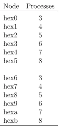
4.6
Processes run on each node
. . . .
54
4.7
Lomb-Scargle computation times
. . . .
77
5.1
Mount Pleasant receivers, calibration scale factors . . . 109
7.1
Results of manual RFI removal
. . . 147
8.1
2016 glitch arrival time estimates . . . 156
8.2
Glitch fitting parameters . . . 157
8.3
Accurate times of the null (
t
0
) at various locations . . . 194
8.4
Times of
t
0
-
t
5
. . . 210
8.5
Glitches of the Vela pulsar . . . 231
8.6
Statistics of ˙
ν
just prior to each glitch . . . 235
A.1 Tracking and recording commands . . . 267
A.2 Tracking and recording commands for other key pulsars . . . 268
A.3 Processing commands . . . 269
A.4 Processing commands - exceptional . . . 270
A.5 Miscellaneous commands . . . 271
A.6 Key files in the pulsar archive . . . 272
B.1 Headings for data recording summary . . . 274
B.2 Historical data recording summary - 2007-2010 . . . 275
xii
LIST OF TABLES
List of Equations
2.3
Differential equation due to magnetic dipole radiation
. . . .
13
2.4
Differential equation relating to pulsar period . . . .
13
2.5
Characteristic age, exact . . . .
15
2.6
Characteristic age, approximation . . . .
15
2.7
Initial period
P
0
. . . .
16
2.13 Dispersion Measure
. . . .
18
2.14 Delay of a pulse by frequency because of dispersion measure . . . .
18
2.15 Taylor’s series . . . .
20
2.16 Taylor’s series for pulsar frequency . . . .
20
2.17 Taylor’s series fit of
y
=
e
x
, degree 4 . . . .
21
2.18 Taylor’s series fit of
y
=
e
x
, degree 10 . . . .
21
2.19 Taylor’s series fit of
y
= 100 sin(
x
), degree 4 . . . .
21
2.20 Taylor’s series fit of
y
= 100 sin(
x
), degree 4 . . . .
21
4.7
Lomb-Scargle . . . .
70
5.1
Log-normal fit of pulsar flux density histogram . . . .
83
5.2
Inverse-square law . . . .
84
5.3
Flux density
∼
distance for Vela . . . .
84
5.4
Distance
∼
flux density for Vela
. . . .
84
5.5
Flux density
∼
distance for a hypothetical FRB . . . .
85
6.1
Timing error given pulse width and signal-to-noise ratio . . . 137
7.1
Timing error for J1644−4559 given pulse width and signal-to-noise ratio . 145
8.3
Moving average . . . 195
8.4
Binning . . . 199
8.6
Braking index . . . 240
Chapter 1
Thesis overview
We begin this thesis with an introduction to pulsar theory that is relevant to this work.
Then we discuss the Vela pulsar (J0835−4510) and the other pulsars that have also
been observed during this study. This is followed by an introduction to the hardware
and software used at the Mount Pleasant and Ceduna observatories. Observed radio
frequency interference is then covered along with a discussion of major statistical tools
used throughout.
Bright and giant pulses observed at both Mount Pleasant and Ceduna observatories
are then discussed.
The paper that appeared in
The Astrophysical Journal
titled
Temporal Evolution of
the Vela Pulsar’s Pulse Profile
is presented along with a postscript discussing updated
data that was gathered since the paper was accepted for publication.
The glitch that was caught live in single-pulse mode at both Mount Pleasant and
Ceduna observatories on 12 December 2016 is then discussed.
The observed
null
,
changes in timing, and flux density are presented. This result appeared in
Nature
.
The conclusion summarises the content and then three appendices are included.
Ap-pendix A provides a list of scripts and commands so that future researchers can continue
pulsar work, Appendix B is a summary table of each day’s recording, including brief
notes, and Appendix C is the paper that appeared in
Nature
on 2018-04-12 titled
Alteration of the magnetosphere of the Vela pulsar during a glitch
.
2
CHAPTER 1. THESIS OVERVIEW
1.1
Notes on style
Scientific writing has a requirement to be precise, however this style also constantly
evolves over the decades. We have used
Scientific Style and Format
(Huth 1994) as
a general guide. Some exceptions and options arose, and so we had to adopt some
specific choices. When deciding, the option making the script
easier to read
was used
as a major guideline. The key selections made were:
•
British English spelling is used throughout.
•
The Oxford comma is always used. Here’s why: “At school I learned from my
teachers, Marie Curie and Albert Einstein.” and
with
the Oxford comma: “At
school I learned from my teachers, Marie Curie, and Albert Einstein.”
•
Double quote marks “ ” have been used not single quotes ‘ ’. This is more
of a United States style, but we’ve adopted it simply to avoid confusion with
apostrophes.
•
If an abbreviation has been used, we write as if the abbreviation has been said
as letters and not its full expansion. For example, FRB as an abbreviation for
Fast Radio Burst, we would say “in the case of an FRB” and not “in the case of
a FRB”.
•
We have adopted the modern style of using the word
data
as singular or plural
depending on context. The singular form
datum
is very rarely used nowadays
(except when explaining why it is not used), and other Latin based words have
followed this path. For example, the words
agenda
and
agendum
. This sentence
would never now be written: “the agenda show that Albert was present”.
•
All pulsar designations are quoted using the J2000 form, but without the leading
“PSR”. For example the Vela pulsar was originally labelled B0833−45 but its
J2000 version is PSR J0835−4510. We write J0835−4510. This looks neater
in tables and provides consistency in layout. Note that care must be taken by
researchers when using on-line searches, as the older names may have been the
only ones used in earlier publications.
•
A number such as 3×10
−
6
would not normally be written as 3000×10
−
9
. However
since pulsar glitch sizes quote
∆
ν
ν
, we always express this in terms of 10
−
9
as this
appears neater in tables, and makes for easier comparisons when reading.
•
We adopt the sign convention of the spectral index to be
S
∝
f
ξ
.
Chapter 2
Introduction
A full introduction of pulsars is not really possible in a single chapter. So for this
work we have focused on key areas that are relevant to later chapters. For an excellent
overall introduction to pulsars,
Handbook of Pulsar Astronomy
(Lorimer and Kramer
2004) is highly recommended.
In summary we briefly cover the formation of pulsars, emission mechanisms, drifting
sub-pulses, nulling, mode changes, bright and giant pulses, characteristic age, braking
index, interstellar medium, dispersion measure, arrival times, timing noise, polynomial
fits and their associated timing artefacts, fast radio bursts, and finally basic glitch
theory.
2.1
Formation of pulsars
In simple terms, at the end of a sufficiently large star’s life, the hydrogen runs out,
nuclear fusion ends, the star collapses, and a Type II supernova occurs. The remains
of the star (
M
≈
1
.
4
M
) collapse further until the neutron degeneracy limit is reached
and as long as the star is not sufficiently large to create a black hole, a neutron star
with a radius of
R
≈
10 km is formed.
The magnetic field at the surface of a typical neutron star is
B
≈
10
12
Gauss,
approx-imately a trillion times that on the surface of the earth. The axis of the magnetic field
is thought to be close to perpendicular to the axis of rotation at the pulsar’s birth,
but then moves slowly to align with the axis of rotation over the lifetime of the pulsar
(Tong and Kou 2017). Once the neutron star is an
aligned rotator
it is no longer visible
as a pulsar.
Initial rotation frequencies of pulsars are not accurately known, but by comparing
char-acteristic age (
τ
c
) with a real known age (e.g. with the Crab pulsar - see Equation 2.7
4
CHAPTER 2. INTRODUCTION
on page 16 and related text), a value of
ν
0
≈
60 Hz can be estimated.
2.2
Emission
The pulsar emission mechanism is still, after nearly 50 years of study, not as well
understood as would be expected. Within a few months of the publication of pulsar
discovery, Gold (1968) stated that rotating neutron stars were the origin of pulsating
radio sources. Despite only a short amount of time for research, this paper is
surpris-ingly accurate to this day. Here are a number of selected quotes from the paper:
“Since the distances are known approximately from interstellar dispersion of the
dif-ferent radio frequencies, it is clear that the emission per unit emitting volume must
be very high; the size of the region emitting any one pulse can, after all, not be much
larger than the distance light travels in the few milliseconds that represents the lengths
of the individual pulses. No such concentration of energy can be visualized except in
the presence of an intense gravitational field.”
“. . . the emission derives its energy from the rotation energy of the star (very likely the
principal remaining energy source), and is a result of relativistic effects in a co-rotating
magnetosphere.”
“A magnetic field of a neutron star may well have a strength of
10
12
gauss at the surface
of the 10 km object.”
“. . . the configuration discussed here may be particularly favourable for the generation
of a coherent radiation mechanism.”
“If this basic picture is the correct one it may be possible to find a slight, but steady,
slowing down of the observed repetition frequencies.”
“Also, one would then suspect that more sources exist with higher rather than lower
2.2. EMISSION
5
to more than 100/s, and the observed periods would seem to represent the slow end of
the distribution.”
This was a very short paper and the majority of the statements proved ultimately to be
correct. Twelve months later Goldreich and Julian (1969) published an influential paper
on the emission process. It has since been shown that the true model is more complex
than originally proposed, however their explanation is still essential in understanding
the pulsar emission mechanism.
Within a magnetised sphere that is rotating there will be an induced electric field.
This electric force acts on the charged particles on the surface of the pulsar and since
this force is many orders of magnitude greater than gravity, these particles are pulled
from the surface. This leads to a plasma surrounding the neutron star and is called
the magnetosphere (Lorimer and Kramer 2004).
This plasma co-rotates with the neutron star out to a point where it reaches the speed
of light. This is called the
light cylinder
and the distance from the centre of the neutron
star to the light cylinder (
R
LC
) is given by:
R
LC
=
cP
2
π
≈
4
.
77
×
10
4
×
P
km
(2.1)
where
P
is the period of the pulsar in seconds and
c
is the speed of light. For Vela
(using 2016 data),
R
LC
= 4262
.
1 km and grows on average by 190 m y
−
1
and shrinks
140 m on each major glitch (see Section 3.1.2 on page 33).
Magnetic field lines that meet within the light cylinder are called
closed field lines
and those that do not meet within the light cylinder are called
open field lines
. The
area where these open field lines leave the surface of the neutron star defines the
polar
cap
.
Radio emission along these open field lines due to curvature radiation is stronger when
the radius of curvature is at its smallest (Komesaroff 1970). This means at the last open
field line, radiation is at its strongest, and emission vanishes along the magnetic axis.
This is known as the
hollow cone
model. Figure 2.1 on page 6 is a reproduction from
Komesaroff (1970) showing how curvature radiation is emitted under this model.
As of this writing there are currently 2613 pulsars in the Australia Telescope National
Facility’s Pulsar Catalogue (Manchester et al. 2005), providing a cross-section of the
wide variety of known pulsars at different states and ages.
[image:29.595.110.463.221.588.2]
(30)