Simulation of the vibrations of a non uniform beam loaded with both a transversely and axially eccentric tip mass

© 2018 WIT Press, www.witpress.com

ISSN: 2046-0546 (paper format), ISSN: 2046-0554 (online), http://www.witpress.com/journals DOI: 10.2495/CMEM-V6-N4-679-690

SIMULATION OF THE VIBRATIONS OF A NON-UNIFORM

BEAM LOADED WITH BOTH A TRANSVERSELY AND

AXIALLY ECCENTRIC TIP MASS

DESMOND ADAIR1 _{& MARTIN JAEGER}2

1_{School of Engineering, Nazarbayev University, Republic of Kazakhstan.} 2_{School of Engineering & ICT, University of Tasmania, Australia.}

ABSTRACT

The main purpose of this work is to employ the Adomian modified decomposition method (AMDM) to calculate free transverse vibrations of non-uniform cantilever beams carrying a transversely and axially eccentric tip mass. The effects of the variable axial force are taken into account here, and Hamilton’s principle and Timoshenko beam theory are used to obtain a single governing non-linear partial differen-tial equation of the system as well as the appropriate boundary conditions. Two product non-linearities result from the analysis and the respective Cauchy products are computed using Adomian polynomials. The use of AMDM to make calculations for such a cantilever beam/tip mass arrangement has not, to the authors’ knowledge, been used before. The obtained analytical results are compared with numerical calculations reported in the literature and good agreement is observed. The qualitative and quantitative knowledge gained from this research is expected to enable the study of the effects of an eccentric tip mass and beam non-uniformity on the vibration of beams for improved dynamic performance. Keywords: Adomian decomposition method, cantilever beam, mechanical vibrations, tip mass

1 INTRODUCTION

The method of solution here is the Adomian modified decomposition method, which is a wide ranging method of solution of problems involving algebraic, differential [11], inte-gro-differential [12] and partial differential equations [13]. Specific to this work, the Adomain decomposition and Adomian modified decomposition method have been used by several groups [14, 15] for uniform and non-uniform beams, starting with either the Euler-Bernoulli or Timoshenko formulations. Mao [14] applied the AMDM to rotating uniform beams and included a centrifugal stiffening term while Adair and Jaeger [15] applied the AMDM to rotating non-uniform beams which also included a centrifugal stiffening term. Yaman [16] has used the Adomian decomposition method to investigate the influence of the orientation effect on the natural frequency of a cantilever beam carrying a tip mass.

In this study we use the computational approach of AMDM to analyze free transverse vibrations of non-uniform cantilever beams carrying a transversely and axially eccentric tip mass. As the beam is assumed to be under the effect of gravity, the spatial variation of axial force is taken into account. The natural frequencies and mode shapes of the beam for three test cases were found and compared with results reported in the literature.

2 MATHEMATICAL FORMULATION

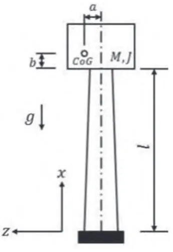
The schematic view of a non-uniform beam with an eccentric tip mass is shown in Fig. 1. The distances a and b are the transverse (z) and axial (x) eccentric values, respectively, CoG is the centre of gravity of the tip mass M and l is the length of the beam. The polar mass moment of inertia of the tip mass around CoG is J and, in this analysis, the axial stretching of the beam due to both gravitational and inertial axial forces is considered.

[image:2.496.163.336.372.623.2]

In order the find the governing equations of motion of the beam, Hamilton’s principle is employed. Every system behaves in such a way to satisfy

δ

t t

e

K U W dt 1

2

0

∫

(

− +

)

= , (1)

where δ is the variation operator, t₁ and t₂ are arbitrary times, K and U are the total kinetic and potential energies of the system respectively and We is the work done by external forces.

For this system, the Euler-Bernoulli assumption that the rotation of cross-sections of the beam is small in comparison to the bending deformation is made. Also it is assumed that the angular distortion due to shear is considered small compared to the bending deformation and can be ignored. Therefore, the beam in question is long and slender with the length much greater than the thickness. With the assumption that the material of the beam is linear elastic, then the overall strain energy can be found from

U EA x u

x

w

x dx EI x

w x

l l

=

( )

∂

∂

+ ∂

∂   

   

  



 

 +

( )

∂ ∂

∫

∫

1 2

1 2

1 2

0

2 2

0

2

2

 

 



 

2

dx, (2)

where A x

( )

and I x

( )

are the area and the second moment of area of the beam’s

cross-sec-tion around the neutral axis and E is Young’s modulus of elasticity of the beam’s material. The total kinetic energy of the system is given as K=K_column+K_mass, where

K A x w

t dx A x

u

t dx

column

l l

=

( )

∂

∂   

 

 +

( )

∂ ∂   

  

∫

∫

1 2

1 2

0

2

0

2

ρ ρ , (3)

K MV J M dw l t

dt a b r

mass= CoG+ CoG = G

(

)



  



 

 +

(

+ +

)

1 2

1 2

1 2

2 2

2

2 2 2



θ ,

 

  

∂ ∂ ∂

(

)



 



 

2_w 2

x t l t,

(4)

+

(

)

∂

∂ ∂

(

)



  +

(

)



  



 

 −

(

2 1

2 2

2 2

bdw l t dt

w

x t l t M

du l t

dt a

du l t

,

, , ,

))

∂

∂ ∂

(

)



  



  

dt w x t l t

2

, .

Here, ρ is the material density of the beam, r_G is the radius of gyration of the tip mass, and



θ and V_CoG are the rotational and translational velocities of the tip mass and its centre of grav-ity, respectively. Here VCoG is obtained using the relative velocity between the tip mass’s

centre of gravity and the point of attachment to the beam.

The virtual work done on the system with the assumption that no viscous damping is pres-ent is

δW_e =δW_g +δW_g

1 2, (5)

where δW_g δW_g

1and 2 are the virtual gravitational work done on the tip mass and the beam,

respectively. The virtual gravitational work done on the system can be written as

δW Mg u l tδ Mgaδ w δ ρ δ

x l t W g A x u x t

g g

l

1 2

0

= −

(

)

− ∂

∂

(

)

  

 

 = −

∫

( )

(

, , , ,

))

dx. (6)

∂ ∂

( )

∂

(

)

∂        − ∂ ∂

(

)

∂

(

)

∂        + ∂ 2 2 2 2

x EI x

w x t

x x N x t

w x t x , , , ∂ ∂

( )

∂

(

)

∂        =

t A x

w x t t

ρ

, . 0 (7)

∂ ∂

( )

∂

(

)

∂        − ∂

(

)

∂ +

( )

=

t A x

u x t t

N x t

x g A x

ρ , , ρ 0 (8),

The variable axial force of the beam, N x t

(

,

)

is defined as

N x t EA x u x t

x

w x t x , , , .

(

)

=

( )

∂

(

)

∂ + ∂

(

)

∂                 1 2 2 (9)

For a long and slender beam, with a small slenderness ratio, the longitudinal inertia is small compared to the restoring force and so

∂

(

)

∂

≈

( )

N x t

x g A x

,

.

ρ (10)

Substitution for the terms N x t

(

,

)

and ∂N x t

(

, /

)

∂x, as defined in eqns (9) and (10) into the expanded form of eqn (7) gives

EI x w x t

x EI x

w x t

x EI x

w

( )

 ∂ _∂

( )

+ _

( )

_′∂

( )

∂ +

( )

′′ ∂ 4 4 3 3 2 2

, , xx t

x g A x

w x t x , ,

( )

∂ −

( )

∂

( )

∂ 2 r (11) −

( )

∂

(

)

∂ ∂

(

)

∂ + ∂

(

)

∂         ∂

(

)

∂

EA x u x t

x

w x t x

w x t x

w x t x

, 2 , , ,

2 2 ₂ 2 1 2          +

( )

∂

(

)

∂ =

ρA x w x t

t 2

2 0

, ,

where the superscript ' mean differentiation w.r.t. x.

According to modal analysis for harmonic free vibration, w x t

(

,

)

and u x t

(

,

)

, can be

sep-arable in space and so eqn (11) can be reduced to

EI x w x

x EI x

w x

x EI x

w x

( )

 d

( )

+ _

( )

_′

( )

+_

( )

_′′

( )

d d d d d 4 4 3 3 2 2

xx g A x

w x x 2 − r

( ) ( )

d d (12) −

( )

( )

( )

+

( )

       

( )

       

EA x u x

x

d w x x w x x w x x d d d d d d d 2 2 2 ₂ 2 1

2 −−ρA x

( )

ω w x

( )

=

2 _0.

The dimensions of the beam in the y and z direction may be given as

d x d x

l d x d

x l d d

( )

=  +

(

−

)

   ′

( )

= ′ +

(

−

)

    ′

0 1 a 1 , 0 1 a 1 , (13)

where α_d =d₁/d₀ , a_d′ = ′ ′d d₁/ ₀; d d₀, ₀′ are the cross-sectional widths at x=0 and d d₁, ₁′ are the cross-sectional widths at x=l. The area and moment of inertia of the beam vary

A x A x l

x

l I x I

x l

d d d d

( )

=  −      −      

( )

= −       − ′ ′

0 1 β 1 β , 0 1 β 1 β

xx l       3 , (14)

where A0 =d d0 0′ and I0 d d0 0 3 ₁₂

= ′ / are the cross-sectional area and moment of inertia at

x=0 , respectively, and β_d =1−α_d, b_d′ = −1 a_d′.

Without loss of generality, the following dimensionless quantities are now introduced.

w l u l x l t T a l a b l b r l r gT l g M l A G G → → → → → → → →

(

φ ψ η τ

ρ

, , , , , , , 2 ,

0

))

→M, where

T l A

EI

= 2 0

0 ρ . λ η λ η λ η λ ρ ω 1 0 2 0 3 2 0 4

0 2 4

0 =

( )

=

( )

=

( )

= EI EI A A EA l EI A l EI

, , , , (15)

, ′ =

( )

     ′ ′′=

( )

     ′′

l1 h l h

0 1 0 EI EI EI

EI (16)

Equation (12) can now be written in the form

d d d d d d d 4 4 1 1 3 3 1 1 2 2 2 1 2 f h h l l f h h l l f h h l l f h h

( )

₊ ′d

( )

₊ ′′

( )

₋

( )

g (17) −

( )

( )

+

( )

       

( )

        − λ λ ψ η η φ η η φ η η φ η η 3 1 2 2 2 ₂ 2 1 2 d d d d d d d

d ωω

λ λ φ η 2 4 1 0

( )

= .

The governing equation, eqn (17), cannot be solved as a closed-form solution and so some approximate approach must be adopted. Here the Adomian modified decomposition method (AMDM) is chosen.

3 ADOMIAN MODIFIED DECOMPOSITION METHOD

The Adomian decomposition method (ADM) is an iterative method, which has proved successful in treating non-linear equations. It is based on the search for a solution in the form of a series in which the non-linear terms are calculated recursively using the Adomian polynomials. The ADM gives the solutions φ η

( )

of eqn (17) in a series form of the infinite sum

φ η

( )

= φ

( )

η

= +∞

∑

j 0 j

, (18)

Substitution of eqn (18) into the linear and nonlinear terms of eqn (17) yields

L R N N

j= j j j

+∞ = +∞

∑

( )

+

∑

( )

−

[

]

−

[ ]

= 0 0 3 1 1 3 1 2 1 2 0

φ η φ η

λ λ ψ φ λ λ φ

where

L= R g

∂ = ′ ∂ ∂ + ′′ ∂ ∂ − ∂ ∂ − d4 4 1 1 3 3 1 1 2 2 2 1 2 2 1 h l l h l l h l l h w

l l

, . (20)

Here L is an invertible operator, which is taken as the highest-order derivative and R is the remainder of the linear operator.

N1

[

ψ φ,

]

in eqn (19) is a product nonlinearity and the respective Cauchy product can be

computed using Adomian polynomials (A_n) as

N A

j

j j j

1

0

0 0

ψ φ, (ψ , ,ψ ;φ , , )φ

[

]

= … … = = +∞

∑

∂ ∂ ∂ ∂ = ∂ ∂ ∂ ∂ = ∂ ∂ ∂ = +∞ = +∞ = +∞ = −

∑

∑

∑∑

ψ η φ η ψ η φ η ψ η φ 2 2 0 0 2 2 0 0 2 j n m m j m j

m j m

∂ ∂η2

.

N2

[ ]

φ in eqn (19) is also a product non-linearity, and accordingly the respective Cauchy

product can be computed using Adomian polynomials (B_n) as

N B

j j j

2 0 0 2 ₂ 2 2 2

φ φ φ

φ η φ η φ η φ η

[ ]

=

(

…

)

= ∂ ∂       ∂ ∂ = ∂ ∂ ∂ ∂       = +∞

∑

, , 22 = (22) j n m m l l j n m l = +∞ = +∞ = +∞ = +∞ = +∞ =

∑

∑

∑

∑

∑

∂ ∂ ∂ ∂ ∂ ∂ = ∂ ∂ 0 2 2

0 0 0

2 2 0 0 φ η φ η φ η φ η + +∞ −

∑

∂ ∂ ∂ ∂ = φ η φ η

l m l

j m j

m l j m

l j m l

= +∞ = = − − −

∑∑

∑

∂ ∂ ∂ ∂ ∂ ∂ 0 0 2 2 0 φ η φ η φ η .

According to the Adomian modified decomposition method (AMDM) the terms φ_j

( )

η in eqn (18) can be expressed as C_j j

η so giving the infinite series

φ η

( )

= η

= +∞

∑

j j j C 0 , (23)

where the unknown coefficients C_j are determined concurrently. Using a similar approach

ψ η

( )

can also be equated to the series

j j j C = +∞

∑

′ 0 h .

Using the linear operator L of Eq. (20) then the inverse operator of L is a 4-fold integral operator defined as

L−

=

_∫∫∫∫

(

⋅ ⋅ ⋅

)

1

0 0 0 0

η η η η

η η η η

d d d d . (24)

Equation (19) can be written as

φ η η η

λ λ η λ λ η

( )

=

( )

− + +   − = +∞ = +∞ = +∞

∑

∑

∑

Φ L R C A B

j j j j j j j j j 1 0 3 1 0 3 1 0 1 2    

where R is now

R j j j C j j C

j

j j

j

j

= ′

(

+

)

(

+

)

(

+

)

+ ′′

(

+

)

(

+

)

= +∞

+

= ∞

∑

∑

l

l h

l l

1

1 0

3 1

1 0

1 2 3 1 2 ₊₊₂hj

(26)

−

(

+

)

−

= ∞

+

= ∞

∑

∑

g j C C

j j

j

j j j

λ λ

η ω

λ λ

η

2

1 0 1

2 4

1 0

1 ,

The Adomian’s polynomials in eqn (25) are found using the standard method [17] for

B_j

₍

φ₀, ,…φ_j

₎

and the generalized method for several variables as reported by Adomian and Rach [18] is used for A_j

₍

ψ₀, ,…ψ_j;φ₀, ,…φ_j

₎

.

The term Φ

( )

η found in eqn (25) is the initial term and defined as

Φ

( )

h = h =f

( )

+f′

( )

h f+ ′′

( )

h + ′′′f

( )

h

=

∑

j j

j

C 0 3

2 3

0 0 0 /2 0 / (27)6

On substituting eqns (23), (26) and (27) into eqn (25), the following is obtained

j j j

C

= ∞

∑

=

( )

+ ′

( )

+ ′′

( )

+ ′′′

( )

0

2 3

0 0 0 2 0 6

h f f h f h / f h /

(28) )

−

+

(

)

(

+

)

(

+

)

+ 

 

 

=

∞ +

∑

j

j

j j j j

0

4

1 2 3 4

η

’ ’’

m j

m m

m m m C m m C

=

+ +

∑

(

+

)

(

+

)

(

+

)

+

(

+

)

(

+

)



 

0

1

1

3 1

1 2

1 2 3 λ 1 2

λ

λ λ

−

(

+

)

−





 + +

  

     

 

+

m 1 g C_m C_m A_j 1B_j

2

2

1 1

2 4

1

3

1

λ λ

ω λ λ

λ λ

The recurrence relation for the coefficients C_j can now be stated and the solution for φ η

( )

can be calculated from eqn (28). The series solution is φ η

( )

= η

= ∞

∑

j j j

C 0

, although all of the

coefficients C_j cannot yet be determined, and thus, the solutions must be approximated by

the truncated series

j n

j j

C

= −

∑

0 1

η , with the successive approximations being φn η η

j n

j j

C

[ ]

= −

( )

=

_∑

0 1

as n

increases and the boundary conditions are met.

Thus φ[ ]1

( )

η =C₀,φ[ ]2

( )

η =φ[ ]1

( )

η +C₁η φ, [ ]3 =φ[ ]2

( )

η +C₂η2 serve as approximate solutions with increasing accuracy as n→ ∞. The three coefficients C_j

(

j=0 1 2 3, , , depend

)

on the boundary equations. In this case, the two coefficients C₀ and C₁ can be chosen as arbitrary constants, and the other two coefficients C₂ and C₃ are stated in terms of the problem parameters or as the functions of the other coefficients.

fr C f C r

n

r n

0 4 0 1 4 1 0 1 2

[ ] [ ]

(

λ

)

+

(

λ

)

= , = , . (29)

For non-trivial solutions, C0 and C1, the frequency equation is given a

f f

f f

n n

n n

10 4 11 4

20 4 21 4

0

[ ] [ ]

[ ] [ ]

(

)

(

)

(

)

(

)

=

λ λ

λ λ

(30)

The ith estimated eigenvalue λ

2i n

( )

[ ] _{corresponding to}

n is obtained from eqn (30), i.e. the ith

estimated dimensionless natural frequency Ω

n i n

i n

( )

[ ]

( )

[ ]

= λ

2 is also obtained and n is

deter-mined by the following equation

Ω_{n i}n Ω_{n i}n

( )

[ ]

( ) −

[ ]

− 1 ≤ε (31)

where Ω_{n i}n

( ) −

[ 1] _{is the ith estimated dimensionless natural frequency corresponding to n}

−1, and ε is a preset sufficiently small value. If eqn (31) is satisfied, then Ω_{n i}n

( )

[ ]

is the ith dimension-less natural frequency Ω_{n i}

( ). By substituting Ωn i

n

( )

[ ]

into eqn (29)

C f

f C r or

r n

n i n

r n

n i n 1

0

1

0 1 2

= −

(

)

(

)

=

[ ]

( )

[ ] [ ]

( )

[ ]

Ω

Ω

, . (32)

and all of the other coefficients C_j can be obtained from recurrence relations. Furthermore, the ith mode shape φ_i[ ]n corresponding to the ith eigenvalue Ω_{n i}n

( )

[ ]

is obtained by

φ_in η η

j n

j i j

C

[ ]

= −

[ ]

( )

=

_∑

0 1

(33)

where Cj i

[ ]

( )

η is C_j

( )

η in which λ₄ is substituted by λ

4( )i and φi n

[ ] _{is the}

ith eigenfunction corresponding to the ith eigenvalue λ

4( )i. By normalizing eqn (33) the ith normalized

eigen-function is defined as

φ η

φ η

φ η η

i

n i

n

i

n _d

[ ]

[ ] [ ]

( )

=

( )

( )

 

 

∫

₀

1 2 (34)

where φ_i[ ]n

( )

η is the ith mode shape function of the beam corresponding to the ith natural

frequency ω_in λ_in ρ ρ

n i n

EI Al EI Al

[ ] [ ]

( )

[ ]

= ₀ / 4 =' ₀ / 4.

4 RESULTS

4.1 Case 1: non-uniform beam

The test case present here is a clamped-free constant width tapered beam (wedge) and the boundary conditions used were

φ

φ

η

φ

η η

0 0 0 0 1 0 1 0

2

2

3

3

( )

=

( )

=

( )

=

( )

=

,d , , .

d

d d

d

d (35)

For the wedge beam α_d’=1,α_d =α β; _d′=0,β_d =β the area and moment of the section can now be written as

A

( )

η =A  +

(

α−

)

η A βη I η I α η I βη

 =

(

−

)

( )

=  +

(

−

)

 =

(

−

0 0 0

3 0

1 1 1 , 1 1 1

))

3,

where β is known as the taper ratio.

In this case the coefficients C0 and C1 were set to zero and the coefficients C2 and C3 are

arbitrary constant. By substituting φn η η

j n

j j

C

[ ]

= −

( )

=

_∑

0 1

into the last two boundary conditions of

eqn (35) the following algebraic equations involving C2 and C3 are obtained

j n

j

n n

j j C f C f

= −

+

[ ] [ ]

∑

(

+

)

(

+

)

=

(

)

+

(

)

=

0 3

2 12 4 2 13 4

1 2 λ λ 0,

(36)

j n

j

n n

j j j C f C f C

= −

+

[ ] [ ]

∑

(

+

)

(

+

)

(

+

)

=

(

)

+

(

)

=

0 4

3 22 4 2 23 4 3

1 2 3 λ λ 0.

and for non-trivial solutions of C₂ and C₃ the frequency equation can be written as

f n f n f n f n

12 4 23 4 22 4 13 4 0

[ ] [ ] [ ] [ ]

(

λ

)

(

λ

)

−

(

λ

)

(

λ

)

= (37)

By solving eqn (37) for n and taking the real root for λ₄ = Ω2_n, it was found that for n=30

Ω Ω

n1 n

30 1

29 _{0 00001}

( )

[ ]

( )

[ ]

− ≤ε= . . (38)

with Ω Ω

n1 n1

30 _{3 517}

( ) ( )

[ ]

≈ = . .

The results for the wedge beam for different taper ratios are compared with those reported by Banerjee et al. [19], as shown in Table 1. The calculated results are in reasonable agreement with those reported by Banerjee et al. [19]. Values for β =0 are not reported by Banerjee

et al. [19] as their method suffered numerical overflow when β =0.

Reasonable agreement was found between the two methods, although the current calcula-tions generally gave slightly larger values. The maximum difference between the two methods was of the order of 1% and occurred for Ω_n3

( ).

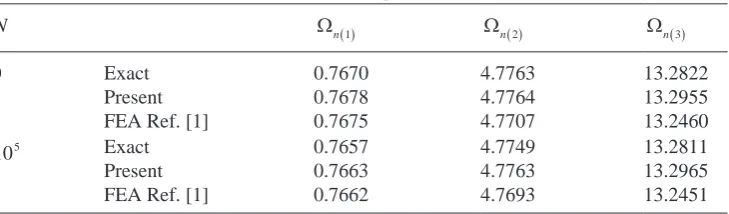
4.2 Case 2: Uniform beam with eccentric tip mass experiencing constant axial force

φ

φ

η

φ

η λ

λ φ

η λ

φ

0 0 0 0 1 1 1

2

2

1 1

3

3 1

2

( )

=

( )

=

( )

= −

( )

+

( )

′

,d , ,

d

d d

d d

d

Mga

dd

d d η

φ

η

2

1 0 +

( )

=

Mg (39)

An exact solution for this eigenvalue problem can be found [1] and is used here for comparison. It can be seen form Table 2 that generally the current calculations give a closer result to the exact solution.

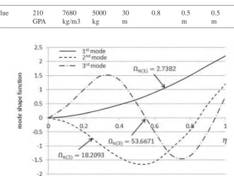
4.3 Case 3: Non-uniform beam with eccentric tip mass and rotary inertia

Here a linearly varying cross section cantilever beam with a both transversely and axially eccentric tip mass with rotary inertia is considered. The beam here is tubular and the physical properties are given in Table 4.

[image:10.496.65.433.84.220.2]

Using the present method, the normalized natural frequencies and mode shapes of the beam are obtained as on Fig. 2.

Table 1: Normalized natural frequencies of a wedge beam.

β Ω_n1

( ) Ωn( )2 Ωn( )3

Current Ref.[21] Current Ref.[21] Current Ref.[21]

0 0.1 0.2 0.3 0.5 0.7 0.9

3.517 3.562 3.612 3.671 3.830 4.090 4.641

– 3.559 3.608 3.667 3.824 4.082 4.631

22.100 21.346 20.639 19.905 18.355 16.667 14.987

– 21.338 20.621 19.881 18.317 16.625 14.931

61.003 59.001 56.293 53.592 47.482 41.005 33.231

[image:10.496.76.433.242.297.2]

– 58.980 56.192 53.322 47.265 40.588 32.833

Table 2: Properties of the uniform beam with tip mass.

Parameter E ρ M l a b r_G D

Value 210

GPa

7680

kg/m3 5000_kg 30_m 1_m 1_m 0.5_m 3_m

Table 3: Normalized natural frequencies of uniform beam.

N Ω_n1

( ) Ωn( )2 Ωn( )3

0 Exact

Present FEA Ref. [1]

0.7670 0.7678 0.7675

4.7763 4.7764 4.7707

13.2822 13.2955 13.2460

105 Exact

Present FEA Ref. [1]

0.7657 0.7663 0.7662

4.7749 4.7763 4.7693

[image:10.496.68.433.531.638.2]

5 CONCLUSIONS

A method has been developed for calculating characteristics of a vibrating non-uniform cantilever beam with an eccentric tip mass. The developed approach is nontrivial and complicated due to the nature of the problem. No exact solution of this general problem is available. Several test cases were performed with quite reasonable agreement between the results of the current approach and those reported in the literature found.

REFERENCES

[1] Malaeke, H. & Moeenfard, H., Analytical modeling of large amplitude free vibration of non-uniform beams carrying a both transversely and axially eccentric tip mass. Journal of Sound and Vibration, 366, pp. 211–229, 2016.

https://doi.org/10.1016/j.jsv.2015.12.003

[2] Prescott, J., Applied elasticity, Dover Publications, New York, 1946.

[3] Goel, R., Vibrations of a beam carrying a concentrated mass. Journal of Applied

Mechanics, 40, pp. 821–822, 1973. https://doi.org/10.1115/1.3423102

[4] Rama Bhat, B., & Wagner, H., Natural frequencies of a uniform cantilever with a tip mass slender in the axial direction. Journal of Sound and Vibration, 45(2), pp. 304–307, 1976. https://doi.org/10.1016/0022-460x(76)90606-4

[image:11.496.74.407.99.349.2]

[5] To, C.W.S., Vibration of a cantilever beam with a base excitation and tip mass. Journal of Sound and Vibration, 172, pp. 289–304, 1994.

Table 4: Physical and geometrical properties of non-uniform beam with eccentric tip mass.

Parameter E ρ M l β a b r_G

Value 210

GPA

7680 kg/m3

5000 kg

30 m

0.8 0.5

m

0.5 m

0.3 m

[6] Auciello, N.M., Transverse vibration of a linearly tapered cantilever beam with tip mass of rotary inertia and eccentricity. Journal of Sound and Vibration, 194, pp. 25–34, 1996. https://doi.org/10.1006/jsvi.1996.0341

[7] Mable, H. & Rogers, C., Transverse vibrations of double-tapered cantilever beams with end support and with end mass. The Journal of the Acoustical Society of America, 55, pp. 986–991, 1974.

https://doi.org/10.1121/1.1914673

[8] Caruntu, D., On bending vibrations of some kinds of variable cross-section using

orthogonal polynomials. Revue Roumaine des Sciences Techniques-Série Délelött

Mécanique Appliquée, 41, pp. 265–272, 1996.

[9] Sanger, D., Transverse vibration of a class of non-uniform beams. Journal of Mechanical Engineering Science, 10, pp. 111–120, 1968.

https://doi.org/10.1243/jmes_jour_1968_010_018_02

[10] Matt, C. F. T., Simulation of the transverse vibrations of a cantilever beam with an eccentric tip mass in the axial direction using integral transforms. Applied Mathematical Modelling, 37, pp. 9338–9354, 2013.

https://doi.org/10.1016/j.apm.2013.04.038

[11] Adomian, G., Nonlinear stochastic system theory and application to physics. Kluwer Academic, Dordrecht, 1988.

[12] Adomian, G. & Rach, R., On composite nonlinearities and the decomposition method.

Journal of Mathematical Analysis and Applications,113(2), pp. 504–509, 1986. https://doi.org/10.1016/0022-247x(86)90321-5

[13] Wazwaz, A. M., Analytic treatment for variable coefficient fourth-order parabolic partial differential equations. Applied Mathematics and Computation, 123, pp. 219–227, 2001. https://doi.org/10.1016/s0096-3003(00)00070-9

[14] Mao, Q., Application of Adomain modified decomposition method to free vibration analysis of rotating beams. Mathematical Problems in Engineering, 2013, pp. 1–10, 2013.

https://doi.org/10.1155/2013/284720

[15] Adair, D. & Jaeger, M., Simulation of tapered rotating beams with centrifugal stiffening using the Adomian decomposition method. Applied Mathematical Modelling, 40, pp. 3230–3241, 2016.

https://doi.org/10.1016/j.apm.2015.09.097

[16] Yaman, M., Adomian decomposition method for solving a cantilever beam of varying orientation with tip mass. Journal of Computational and Nonlinear Dynamics, 2, pp. 52–57, 2007.

https://doi.org/10.1115/1.2389167

[17] Adomian, G., A new approach to nonlinear partial differential equations. Journal of Mathematical Analysis and Applications, 102(2), pp. 420–434, 1984.

https://doi.org/10.1016/0022-247x(84)90182-3

[18] Adomian, G. & Rach, R., Generalization of Adomian polynomials to functions of several variables. Computers & Mathematics with Applications, 24(5/6), pp. 11–24, 1992.

https://doi.org/10.1016/0898-1221(92)90037-i