Theses
Thesis/Dissertation Collections
5-1-2010
Scalable data clustering using GPUs
Andrew D. Pangborn
Follow this and additional works at:
http://scholarworks.rit.edu/theses
This Thesis is brought to you for free and open access by the Thesis/Dissertation Collections at RIT Scholar Works. It has been accepted for inclusion in Theses by an authorized administrator of RIT Scholar Works. For more information, please [email protected].
Recommended Citation
by
Andrew D. Pangborn
A Thesis Submitted in Partial Fulfillment of the Requirements for the Degree of Master of Science in Computer Engineering
Supervised by
Associate Professor Dr. Muhammad Shaaban Department of Computer Engineering
Kate Gleason College of Engineering Rochester Institute of Technology
Rochester, New York May 2010
Approved by:
Dr. Muhammad Shaaban, Associate Professor
Thesis Advisor, Department of Computer Engineering
Dr. Gregor von Laszewski, Assistant Director of Cloud Computing
Committee Member, Pervasive Technology Institute, Indiana University
Dr. Roy Melton, Lecturer
Committee Member, Department of Computer Engineering
Dr. James Cavenaugh, Postdoctoral Fellow
Rochester Institute of Technology Kate Gleason College of Engineering
Title:
Scalable Data Clustering using Graphics Processing Units
I, Andrew D. Pangborn, hereby grant permission to the Wallace Memorial Library to reproduce my thesis in whole or part.
Andrew D. Pangborn
Dedication
Acknowledgments
I am grateful for Gregor von Laszewski who sparked my interest in
paral-lel computing, inspired this thesis project, and provided continual research
guidance and professional advice. Special thanks to Dr. James Cavenaugh
and his colleagues in the Flowgating group at the University of Rochester
Center of Vaccine Biology and Immunology for their expertise and data.
Finally, I would like to thank my advisors Dr. Muhammad Shaaban and
Dr. Roy Melton whose instruction and guidance in the fields of computer
architecture and scientific programming has been invaluable with this thesis
and my own development as a professional.
Abstract
Scalable Data Clustering using GPUs
Andrew D. Pangborn
Supervising Professor: Dr. Muhammad Shaaban
Flow cytometry is a mainstay technology used by biologists and immunologists for counting, sort-ing, and analyzing cells suspended in a fluid. Like many modern scientific applications, flow cytom-etry produces massive amounts of data, which must be clustered in order to be useful. Conventional analysis of flow cytometry data uses manual sequential bivariate gating. However, this technique is limited in the quantity, quality, and speed of analyses produced. Unsupervised multivariate cluster-ing techniques have shown promise for produccluster-ing sound statistical analyses of flow cytometry data in previous research.
The computational demands of multivariate clustering grow rapidly, and therefore processing large data sets, like those found in flow cytometry data, is very time consuming on a single CPU. Fortunately these techniques lend themselves naturally to large scale parallel processing. To address the computational demands, graphics processing units, specifically NVIDIA’s CUDA framework and Tesla architecture, were investigated as a low-cost, high performance solution to a number of clustering algorithms.
C-means and Expectation Maximization with Gaussian mixture models were implemented us-ing the CUDA framework. The algorithm implementations use a hybrid of CUDA, OpenMP, and MPI to scale to many GPUs on multiple nodes in a high performance computing environment. This framework is envisioned as part of a larger cloud-based workflow service where biologists can apply multiple algorithms and parameter sweeps to their data sets and quickly receive a thorough set of results that can be further analyzed by experts.
Contents
Dedication . . . iii
Acknowledgments . . . iv
Abstract . . . v
1 Introduction. . . 1
2 Background . . . 3
2.1 Data Clustering . . . 3
2.1.1 Types of Data clustering . . . 3
2.2 Flow Cytometry . . . 5
2.2.1 Data . . . 6
2.2.2 Bivariate Gating Analysis . . . 7
2.2.3 Multivariate Analysis . . . 7
2.3 Workflow . . . 8
2.3.1 Data Extraction . . . 9
2.3.2 Data Preparation . . . 10
2.3.3 Clustering . . . 11
2.4 GPGPU . . . 12
2.4.1 CUDA . . . 14
3 Supporting Work . . . 21
3.1 Algorithms . . . 21
3.1.1 C Means . . . 21
3.1.2 Gaussian Mixture Models . . . 22
3.2 Data Clustering on GPGPU . . . 25
4 Parallel Algorithm Implementations . . . 28
4.1 Parallel Implementation Architecture . . . 28
4.2 C-means . . . 31
4.2.1 Data Organization . . . 34
4.2.3 Membership kernel . . . 36
4.2.4 Update Centers kernel . . . 39
4.2.5 Comparison to prior work . . . 44
4.3 Expectation Maximization . . . 45
4.3.1 Data organization . . . 46
4.3.2 Initialization . . . 48
4.3.3 E-step . . . 48
4.3.4 M-step . . . 49
4.3.5 Combine Gaussians . . . 54
4.3.6 Summary . . . 54
5 Results. . . 56
5.1 Testing Environment . . . 56
5.2 Resource Utilization . . . 57
5.3 Single Node Performance . . . 60
5.3.1 Algorithm Complexity . . . 60
5.3.2 Speedup . . . 69
5.4 Comparison to prior work . . . 80
5.4.1 C-means . . . 80
5.4.2 EM with Gaussians . . . 82
5.5 Horizontal Scalability . . . 83
5.5.1 Fixed Problem Size Scalability . . . 84
5.5.2 Time-constrained Scaling . . . 90
5.6 Results - Iris Data . . . 92
5.7 Verification - Synthetic Data . . . 96
5.8 Flow Cytometry Data . . . 102
6 Conclusion . . . 109
7 Future Work . . . 111
List of Tables
4.1 UpdateCenters vs. CUBLAS SGEMM . . . 44
5.1 C-means Kernel Resource Usage . . . 58
5.2 C-means Kernel FCS File Resource Usage . . . 59
5.3 EM Kernel Resource Usage . . . 59
5.4 EM Kernel Shared Memory Usage . . . 59
5.5 EM Kernel Performance with Different Threads per Block . . . 60
5.6 Comparison of C-means Execution time (ms) to [1] . . . 80
5.7 Comparison of C-means Execution time (ms) to [2] . . . 81
5.8 Comparison of EM Kernel time (ms) to [3] . . . 82
5.9 Comparison of EM time (s) to [4] . . . 83
5.10 C-means Speedup Summary . . . 88
5.11 Expectation Maximization Speedup Summary . . . 90
5.12 Scaled Speedup Summary: M=100, D=24, N=50K per node . . . 94
5.13 Iris Data Cluster Sizes . . . 94
5.14 Iris Data Cluster Means . . . 96
5.15 Synthetic Data Test 1: C-means . . . 98
5.16 Synthetic Data Test 1: Gaussians . . . 99
5.17 Test #2 Dataset . . . 100
5.18 Test #2 C-means Clustering Summary . . . 101
5.19 Test #2 EM Gaussian Clustering Summary . . . 101
List of Figures
2.1 Taxonomy of Clustering Algorithms [5] . . . 4
2.2 Hydrodynamic Focusing of Particles in a Flow Cytometer [6] . . . 6
2.3 Bivariate Scatter Plot [6] . . . 8
2.4 Flow Cytometry Workflow . . . 9
2.5 NVIDIA Tesla G80/G92 GPU Architecture [7] . . . 13
2.6 NVIDIA CUDA Architecture Overview [8] . . . 15
2.7 CUDA Multiprocessor Architecture [9] . . . 16
2.8 CUDA Thread Hierarchy [9] . . . 16
2.9 CUDA Memory Model [9] . . . 18
3.1 High-Level Clustering Procedure [10] . . . 25
4.1 Process Hierarchy . . . 29
4.2 Communication and Reduction Hierarchy . . . 30
4.3 Pseudo-Code for the Program Flow of C-means on the Host . . . 33
4.4 Pseudo-code for Distance Kernel . . . 35
4.5 Effect of Grid Size on Distance and Membership Kernels . . . 36
4.6 Pseudo-code for Membership Kernel . . . 37
4.7 C-means Partition Camping . . . 38
4.8 Pseudo-code for Membership Kernel . . . 39
4.9 Pseudo-code for UpdateCenters kernel . . . 41
4.10 CUBLAS implementation of Cluster Centers . . . 43
4.11 CUBLAS SGEMM Performance on 2 data sets . . . 43
4.12 Gaussian mixture model data structure . . . 47
4.13 E-step log-likelihood kernel pseudo-code . . . 49
4.14 E-step membership kernel pseudo-code . . . 50
4.15 M-step host pseudo-code . . . 51
4.16 M-stepnpseudo-code . . . 51
4.17 M-stepµpseudo-code . . . 52
4.18 M-step covariance pseudo-code . . . 53
5.2 C-means GPU kernel scalability: N . . . 62
5.3 Expectation Maximization Scalability: N . . . 63
5.4 Breakdown of Execution Time for C-means and EM: N . . . 64
5.5 Naive C-means Scalability: M . . . 65
5.6 Optimized C-means Scalability: M . . . 65
5.7 Expectation Maximization Scalability: M . . . 66
5.8 Breakdown of execution time for C-means and EM: M . . . 66
5.9 C-means Scalability: D . . . 68
5.10 Expectation Maximization Scalability: D . . . 68
5.11 Breakdown of execution time for C-means and EM: D . . . 69
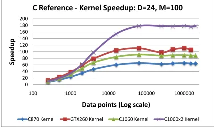
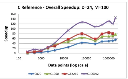
5.12 C-means Kernel Speedup vs. events: C reference version . . . 70
5.13 C-means Speedup vs. events: C reference version . . . 70
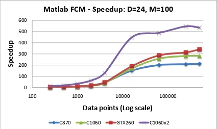
5.14 C-means Speedup vs. events: MATLAB fcm . . . 72
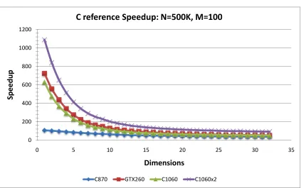
5.15 C-means Speedup vs. dimension: C reference . . . 72
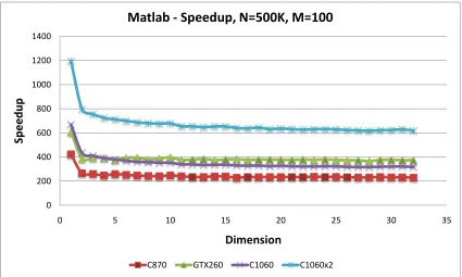
5.16 C-means Speedup vs. dimension: MATLAB . . . 73
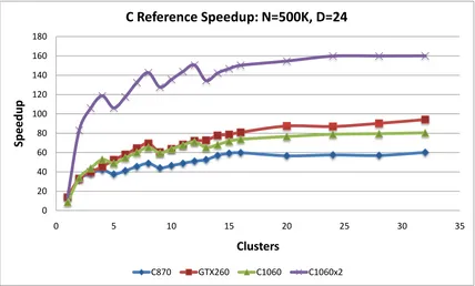
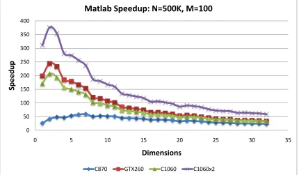
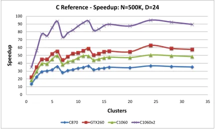
5.17 C-means Speedup vs. clusters: C reference . . . 74
5.18 C-means Speedup vs. clusters: MATLAB . . . 74
5.19 EM Kernel Speedup vs. events: C reference version . . . 75
5.20 EM Speedup vs. events: C reference version . . . 75
5.21 EM Speedup vs. events: MATLAB Gmdistribution.fit EM . . . 77
5.22 EM Speedup vs. dimension: C reference . . . 77
5.23 EM Speedup vs. dimension: MATLAB . . . 78
5.24 EM Speedup vs. clusters: C reference . . . 79
5.25 EM Speedup vs. clusters: MATLAB . . . 79
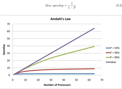
5.26 Amdahl’s law with various degrees of parallelization . . . 84
5.27 C-means Strong Scaling Speedup . . . 85
5.28 C-means Strong Scaling Time Breakdown . . . 86
5.29 C-means Strong Scaling Speedup . . . 87
5.30 EM Strong Scaling Speedup . . . 89
5.31 EM Strong Scaling Time Breakdown . . . 89
5.32 C-means execution time with constant problem size per node . . . 91
5.33 EM execution time with constant problem size per node . . . 92
5.34 C-means Scaled Speedup . . . 93
5.35 EM Scaled Speedup . . . 93
5.36 Iris Data Set [11] . . . 95
5.37 Test 2 Gaussian Mixture Data . . . 100
5.39 Density Plot of Forward Scatter vs. Side Scatter with a Physical Mixture of 50%
Human Blood Cells and 50% Mouse Blood Cells . . . 104 5.40 Density Plot of an electronic mixture (bottom) of Human blood cells (top-left) and
Chapter 1
Introduction
Science and business applications often produce massive data sets. This immense amount of data
must be classified into meaningful subsets for data analysts and scientists to draw meaningful con-clusions. Data clustering is the broad field of statistical analysis that groups similar objects into
relatively homogenous sets called clusters. Data clustering has a history in a wide variety of fields,
such as data mining, machine learning, geology, astronomy, and bioinformatics, to name a few [5] [12]. The nature of the data similarity varies significantly from one application and data set to
an-other. Therefore no single data clustering algorithm is superior to all others in every instance. As such, there has been extensive research and a myriad of clustering techniques developed in the past
50 to 60 years [12].
Flow cytometry is a mainstay technology used in immunology and other clinical and biological research areas such as DNA analysis, genotyping, phenotyping, and cell function analysis. It is
used to gather information about the physical and chemical characteristics of a population of cells.
Flow cytometers produce ad-length multidimensional data vector of floating point values for every event (usually a cell) in a sample, wheredindicates the number of photo-sensitive sensors installed.
Typical samples have on the order of106 events with upwards of 24 dimensions (and this number
is expected to continue increasing as flow cytometer technology improves). This massive amount of data must then be clustered in order for biologists to draw meaningful conclusions about the
characteristics of the sample.
Sequential bivariate gating is the approach traditionally followed by biologists for clustering and analyzing flow cytometry data. Two dimensions of the data are analyzed at a time with a scatter
plot. Clusters are then manually drawn around populations of cells by a technique called gating.
The data sets are typically diffuse and clusters are not always well-defined and distinct; therefore gating requires experience and expert knowledge about the data and the dimensions involved.
Un-fortunately this process is time consuming, cumbersome, and in-exact. Unpublished research by
the University of Rochester Center for Vaccine Biology and Immunology suggests that results can vary by as much as an order of magnitude between experienced immunologists on a difficult data
set. Therefore both the number and quality of the analyses produced by sequential bivariate gating
with manual gating.
Multivariate data clustering techniques have been around for decades; however their application
to the field of flow cytometry has been limited. There has been a recent surge in research activity over the past few years applying multivariate data clustering to flow cytometry data.
Multivari-ate techniques have the potential to use the full multidimensional nature of the data, to find cell
populations of interest (that are difficult to isolate with sequential bivariate gating), and to allow analysts to make more sound statistical inferences from the results. Flow cytometry data sets are
complex, containing millions of events, dozens of dimensions, and potentially hundreds of natural
clusters. Unsupervised multivariate clustering techniques are computationally intensive, and the computational demands grow rapidly as the number of clusters, events, and dimensions increase.
This makes it very time consuming to analyze a flow cytometry data set thoroughly using a single
general purpose processor. Fortunately, many clustering techniques lend themselves nicely to large scale parallel processing.
In this thesis NVIDIA’s CUDA framework for general purpose computing on graphics pro-cessing units (GPGPU) was investigated as a low cost, high performance solution to address the
computational demands of unsupervised multivariate data clustering for flow cytometry [13]. The
existing work on data clustering algorithms using GPGPU has been limited in the algorithms imple-mented, the scalability of such algorithms (such as using multiple GPUs), and lack of optimization
specifically for the flow cytometry problem. Two unsupervised multivariate clustering algorithms,
C-means and Expectation Maximization with Gaussian mixture models, were implemented using CUDA and the Tesla architecture. Multiple GPUs on a single machine are leveraged using shared
memory and threading with OpenMP. The parallelism is expanded to support GPUs spread across
multiple nodes in a high-performance computing environment using MPI. Functionality is verified for all methods using synthetic data. Real flow cytometry data sets are used to assess the accuracy
and quality of results. The performance of sequential, single GPU, and multiple GPU
implementa-tions are compared in detail.
The remainder of this thesis is organized as follows. Chapter 2 provides an overview of data
clustering, flow cytometry, modern GPU architectures, and the CUDA framework. After motivating
the use of GPUs for data clustering, Chapter 3 discusses the specific clustering algorithms imple-mented in the thesis followed by previous GPGPU efforts with clustering algorithms. Chapter 4
provides implementation details for the parallel clustering algorithms and discusses improvements
over previous work. Chapter 5 analyzes results for the parallel clustering algorithms using a va-riety of different performance metrics. Finally, Chapters 6 and 7 conclude the thesis and provide
Chapter 2
Background
This chapter begins with an overview of data clustering and discusses the specific classes of
cluster-ing algorithms used in this thesis. The basics of flow cytometry and the characteristics of the data are covered to motivate the use of GPUs for high performance clustering of such data sets. Finally
the chapter provides an overview of the NVIDIA Tesla GPU architecture and CUDA framework
such that the reader can understand the implementation descriptions in Chapter 4.
2.1
Data Clustering
Data clustering is a statistical method for grouping of similar objects into related or homogeneous
sets, called clusters. There are a myriad of scientific fields and commercial applications that generate
immense amounts of data, ranging from high energy particle physics at CERN to the buying habits of consumers at grocery stores. In any case, the objective is to group related data together so
that analysts can draw meaningful conclusions from the data. The goal of data mining as well
as the size and nature of the data varies tremendously from one field to another, and even from one data set to another in a given field. As such, there has been a wide variety of data clustering
techniques developed over the past 60+ years. No single data clustering algorithm is sufficient for
all applications.
2.1.1 Types of Data clustering
An exhaustive discussion of data clustering techniques is beyond the scope of this thesis. However, this section provides an overview of the different types of data clustering algorithms that are
ac-celerated by GPUs in this thesis. For a more thorough review of data clustering techniques please
consult [5] and [12].
Data analysis can be dichotomized into two broad efforts — exploratory or confirmatory [5].
The former case attempts to gain insight into the contents of the data and form hypotheses, whereas
the former case, whereas the latter cases are categorized as classification techniques. Flow
cytom-etry has a wide variety of applications that fall into both categories. Regardless of the technique
involved, data clustering algorithms face the same questions. How many meaningful clusters exist in the data? How well does the data fit the cluster configuration or model? Are all of the natural
clusters being exposed? What does each cluster represent? While philosophically simple, in
prac-tice these are difficult problems, and as such these sorts of questions have plagued researchers for decades and are the reason why data clustering remains such a challenging and computationally
intensive problem.
Many popular data clustering techniques have a combinatorial increase in computational time complexity as the number of dimensions, the number of vectors, and the number of clusters
in-crease. The nature of the data in flow cytometry, with millions of events, over 20 dimensions, and
potentially hundreds of natural clusters, make unsupervised data clustering both difficult and very computationally demanding.
Figure 2.1: Taxonomy of Clustering Algorithms [5]
Among the unsupervised (exploratory) clustering techniques are many subcategories. Figure 2.1 displays a taxonomy of clustering techniques from Jainet al. [5]. In this thesis three different
types of data clustering are investigated.
• Square error: Fuzzy C-means
• Mixture Resolving: EM with Gaussians
The first is a partitioning method that minimizes square error [5] — although some literature
classifies it as acenter-basedmethod [12]. In center-based techniques, a configuration withk
clus-ters has k d-dimensional cluster centers. The most common center-based clustering method is the k-means algorithm. Events in the data set are grouped into the cluster whose center is closest.
Cen-ters are then recomputed based upon their members. The center-based methods fall into the category
of squared error clustering because it is minimizing the distance (error) between the data vectors and the nearest cluster. Fuzzy K-means [14] (typically called C-means in the data clustering literature)
is an extension of K-means that computes membership values for each cluster as opposed to a hard
classification of each vector to a single cluster. C-means is implemented in this thesis and will be discussed in more detail in the following chapter.
The next method is amixture resolving(model-based) partitioning method. It assumes that the
data are composed of a collection (mixture) of different distributions. The model-based algorithm investigated in this thesis is expectation maximization (EM) with Gaussians. It is a two-step iterative
clustering algorithm, where the first step of each iteration maps the probability of each individual data point to the current models, and the second stage updates the statistical parameters of the
models based upon the new probabilities.
Agglomerative hierarchical clusteringworks by computing pairwise distances between all
ob-jects and then iteratively combining the most similar obob-jects. The similarity measure varies
sig-nificantly from one implementation to another. This thesis does not use hierarchical clustering to
cluster all of the data. Instead it combines hierarchical clustering with the Gaussian Mixture Model approach. In this case, the Gaussian models are combined rather than the individual data elements
— in other words, the clusters are being clustered. The similarity measure is based upon the
covari-ances and means of the Gaussian distributions.
2.2
Flow Cytometry
Flow cytometry is a process for studying the physical and chemical characteristics of a group of particles (usually cells) suspended in a fluid. The system contains three major components —
fluidics,optics, andelectronics. The fluidics system is responsible for creating a narrow stream of
particles that pass through the optics by a technique known as hydrodynamic focusing (see Figure 2.2) [15]. Optics consist of one or more lasers of different wavelengths. Lenses, mirrors, and
filters direct the scattered light to different photo-sensitive electronic detectors as seen in Figure
2.2. The particles (typically cells) pass through a focused laser beam at a rate of thousands per second. Light hits the cell and is refracted (scattered) in all directions. Forward scatter information
can describe physical characteristics of the particle, such as cell size. Other light gets scattered to
use fluorescently labeled antibodies. The cell samples are doped with various fluorescent reagents,
which bind to certain types of cells, to act as indicators. When light hits the fluorescent molecules,
they become excited and emit light at a particular wavelength [6]. Different colors of light will be emitted depending upon which fluorescent markers are attached to the cell, and the corresponding
[image:18.612.158.465.184.392.2]light emission is picked up by a series of detectors. [15]
Figure 2.2: Hydrodynamic Focusing of Particles in a Flow Cytometer [6]
2.2.1 Data
The information from all of the different detectors forms a data vector for each event — a particle
or cell passing through the laser. Current optical flow cytometers can have as many as 20 detectors. Emerging state of the art instruments such as CyTOF [16] currently have 35 dimensions and are
expected to grow to 50 to 60 dimensions in the near future. Flow cytometers produce large data
sets on the order of 105–106 events with tens of dimensions. The computational complexity of both algorithms grows combinatorially with respect to the dimensions of the input and the number
of clusters. For example, 1 million events with 24 dimensions and 100 clusters would require 2.4
billion distance calculations per iteration of C-means. These large data sets motivate the use of high performance computational architectures such as GPU co-processors.
In addition to the raw data there are headers to indicate to which color/sensor the dimensions
correspond, and compensation information for the different channels. Annotation information for the cell sample can also be present. The industry uses the flow cytometry standard (FCS) file format
2.2.2 Bivariate Gating Analysis
Analyzing multivariate data with more than a few dimensions is challenging because it is difficult to
visualize or summarize the data. Bivariate gating is the traditional and most mature, albeit limited, approach used in the flow cytometry field for analyzing data. Histograms plot a single dimension of
the data versus the frequency of a range in the cell population. It is fairly reasonable for an operator
to observe 10-20 histogram plots, but this visualization technique does not allow the analyst to observe all of the overlapping, but naturally distinct, cell populations in the data. Instead, two
dimensions at a time are analyzed in a scatter plot to expose more distinct cell populations. Figure
2.3 shows a simple scatter plot of the forward and side refraction data for a flow cytometry sample and their corresponding histograms. The different colors in the plot denote the natural clusters, (in
this case, different types of cells such as lymphocytes, monocytes, and neutrophils) [6]. Naturally
the cell type for each event would not be known a priori with real data, and therefore the analyst would group the blobs of cells in the scatter plot into distinct clusters. Expert knowledge must then
be used by the immunologist studying the data to determine to what each cluster corresponds based
upon the dimension and location of the clusters in the plot. For non-trivial analyses it is necessary to cluster the data iteratively rather than to use single scatter plots. Bins are drawn around cell
populations, and then cells within a particular bin are further analyzed using different dimensions. This technique is known as sequential bivariate gating.
There are many software packages available for flow cytometry, such as FlowJo [18] and WebFlow
[19]. However, most of this software focuses on bivariate analysis techniques. Services provided include data management and organization, statistical analysis, gating, and visualization.
2.2.3 Multivariate Analysis
The previous section discussed how moving from one dimension to two dimensions for analysis
exposed many more natural clusters in the data. However with data containing upwards of 24
dimensions, there is still a lot of potential information in the data that may not be exposed by bivariate techniques. As the number of colors increases, the parameter space for bivariate analysis
grows rapidly. While a simple experiment with 6 colors has only 64 possible boolean parameters, a
20-color experiment has on the order of106.
Using an iterative sequential bivariate technique with multiple scatter plots and different
combi-nations of dimensions allows the analyst to see a lot of different characteristics in the cell population.
However, the number of different ways of analyzing the dimensions two at a time grows combina-torially, and consistent, reliable data analysis is difficult for manual operators. Very slight changes
in the binning in one iteration of the sequential bivariate analysis can also have a large impact on
the final result.
Figure 2.3: Bivariate Scatter Plot [6]
flow cytometry data. Despite the presence of automatic multivariate clustering in the flow cytometry
literature for nearly 25 years [20] [21] [22], it has had little effect on the flow cytometry community in practice. However, some recent research efforts such as FLAME [23] and Lo et. al [24] have
shown promise for the use of automated multivariate clustering for flow cytometry with biological
case studies. Only recently have any multivariate flow cytometry data analysis tools began to emerge for widespread use, such as Immport [25], and FlowCore [26]. Many of the methods have high
computational complexity and it is difficult for researchers to analyze flow data using these methods
in a timely fashion on a CPU.
2.3
Workflow
So far Chapter 2 has discussed the characteristics of flow cytometry data and a brief overview of an individual analysis of the data. Although this thesis focuses on the computational bottleneck of
unsupervised multivariate clustering, the workflow for analyzing flow data generally requires more than a single clustering of the raw data from the flow cytometer. This section describes the
pre-processing steps required before the flow data set is clustered on the GPU, the clustering itself, and
A suite of Python scripts were developed for the processing stages of the workflow to
pre-pare flow data for clustering by the CUDA program. Additional scripts generate plots from the
clustering result files. These scripts utilize NumPy, which is the de-facto open-source library for working with matrices and numeric processing in Python, and Matplotlib for plotting.
Read FCS File ↓
Extract Machine Info, Raw Data ↓
Censor Saturated Values (optional) ↓
Compensate Data ↓
Transform Fluorescent Variables ↓
Perform Clustering l
Statistical Summary, Visualize Result l
Expert Analysis
Figure 2.4: Flow Cytometry Workflow
2.3.1 Data Extraction
Data collected by flow cytometers are stored in the Flow Cytometry Standard (fcs) format. It
con-tains a header, a text portion with meta-data (instrument details, compensation, patient/sample
in-formation, etc.), and the raw data. The complete details of the FCS 3.1 format are maintained by the International Society for Advancement of Cytometry [17].
The first script in the workflow extracts the relevant information from the binary FCS file. There
are two key pieces that must be extracted from the FCS file for the clustering workflow — the SPILL variable information (found in the TEXT portion of the FCS file) and the raw data (found in the
DATA portion of the fcs file). SPILL contains a list of the fluorescent variables as well as a matrix
of spillover information. This information is used to try to negate the effects of fluorescent spillover (an inherent side-effect of the optics used in the machines) from one channel to another. The process
of negating the spillover effect is called data compensation. If compensation is performed properly
2.3.2 Data Preparation
After the data and spillover information have been extracted, the data are filtered, compensated,
and transformed. Filtering removes data points where the light detectors have been saturated (equal to the maximum value of the ADC on the instrument). Due to saturation these values cannot be
accurately measured. They are removed before clustering to prevent results being skewed by
val-ues accumulated on an artificial axis (the upper-bound of the machine’s measuring capability). A high percentage of saturated values indicates that the machine voltages and gains are not properly
configured.
The next step is to compensate the data using the spillover matrix. Often times the spillover is not contained within the FCS file itself, but provided separately — the script supports both scenarios.
The raw data (dimensionalityN×D) found in the FCS file are the product of the compensated data
(the data of interest) and the spillover matrix (dimensionality D ×D). Thus the compensated
data can be calculated by multiplying the raw data by the inverse of the spillover matrix, (i.e. the
compensation matrix).
raw =compensated∗spillover (2.1)
compensated=raw∗spillover−1 (2.2)
Transformation is the final step. Flow data contain two main classes of variables — scatter and
fluorescent. Scatter information measures how much the light scatters (or spreads) when the laser hits the cell. This results in relatively linear data and does not require any transformation (nor is
it included in the compensation). These values range from 0 to218−1, (the machine has an 18-bit ADC), for the data files used in this thesis from the University of Rochester Center of Vaccine
Biology and Immunology. The fluorescent variables are the key biological indicators and tend to
exhibit log-like responses. The two unsupervised data clustering methods used in this thesis rely on the dimensions in question to be weighted relatively evenly in order to work properly. Therefore all
fluorescent dimensions are transformed from a log-like scale to a linear scale, and then the data set
is rescaled to match the range of the scatter variables. Manual gating software effectively analyzes data the same way since fluorescent variables are plotted on a log scale.
The Logicle (a form of the biexponential) transformation [27] is often referenced in flow
cytom-etry research and used in popular flow cytomcytom-etry tools such as FlowJo [18]. This transformation addresses the problem of log data with both negative and positive values and the often non-uniform
shapes encountered in flow data. The transformation is linear near zero and becomes logarithmic for
larger values, resulting in a relatively linear display of the originally log-like data across the entire range.
transformation implementation is based on a MATLAB application written by Jonathan Rebhahn
at the University of Rochester. The data can be written to a comma-separated-value (CSV) file
after all data pre-processing is complete. CSV is a very generic and portable format that allows the clustering applications to maintain a simple interface for any type of floating-point input data.
It also allows the data to be interpreted by other programs such as MATLAB or plotting utilities.
However, processing large CSV files is computationally intensive, which can be prohibitive for parallel speedup (assuming the I/O is not parallel). Therefore the scripts also output to a simple
binary file format. Using binary files reduced I/O time for the CUDA programs by an order of
magnitude.
The first four bytes of the binary file are a 32-bit integer encoded in little endian that stores the
number of events in the file. The next four bytes are an integer for the number of dimensions. The
remaining values are single-precision (32-bit) IEEE 754 floating-point numbers which comprise all of the data in row-major order; consecutive values are from the same event, not the same dimension.
A Python script was written that can transform from CSV to this simple binary format and vice versa. The clustering algorithms assume any files with a.binextension are binary files, and anything
else it attempts to parse as CSV file.
2.3.3 Clustering
After the preprocessing of the data set is complete, clustering begins. A one-to-many relationship
exists between a particular data set and the clustering analyses that can be performed on it. There are two main sources of different clustering analyses. First, no single clustering algorithm has
been shown to be universally superior to all others for all purposes, and different algorithms can
be expected to give different clusters and different numbers of clusters. Depending on the specific objectives of the analysis, different algorithms may be chosen. For example, one algorithm may be
good at exploratory analysis of the data, able to locate very small clusters out of the entire data set,
while another may be good at consistently profiling larger clusters — which is useful for inference across data sets. While this thesis focuses on only two clustering algorithms, many more may be
used.
Secondly, for any particular clustering algorithm it may be desirable to do parameter sweeps (such as varying the number of starting clusters, or the parameters used by information criteria such
as MDL) as well as sensitivity analyses. Using many different algorithms, each with many different
starting parameters, results in an analysis with dozens or even hundreds of clusterings. Finally, intuitive visualization of the results is necessary in order for experts to gauge the quality of the
results and to determine the biological implications of the results (i.e. to what cells do the clusters
correspond).
A very important, yet under-developed, aspect of flow cytometry research is good statistical
across samples. Here the one-to-many relationship between a particular data set and the clustering
analyses is expanded to a many-to-many relationship with multiple data sets, each with various
clusterings. As previously mentioned, even a single clustering algorithm can be slow on a single CPU. Clearly there is a great need to have accelerated algorithms in order for the workflow to be
feasible in reasonable time.
2.4
GPGPU
Traditional von Neumann general purpose processor architectures support only a single active thread
of execution. Sequencing of operations is quite easy with this architecture — however concurrency is difficult. While the capabilities of general purpose processors to exploit parallelism have
im-proved significantly throughout the years due to techniques such as the Tomasulo algorithm,
super-scalar dispatching, vector instructions, symmetric multi-threading, and multiple-core technologies, they still remain limited to a relatively small number of concurrent threads. In addition, a significant
portion of on-chip resources are dedicated to decoding massive instruction sets for general purpose
computing, branching, synchronization, pipelining, and caching. The resources available for raw floating point computations (used heavily in clustering) are comparatively limited. Effectively
meet-ing the computmeet-ing requirements of scientific applications usmeet-ing general purpose processors often requires hundreds if not thousands of processors.
Graphics processing units (GPUs) have evolved from simple fixed function co-processors in the
graphics pipeline to programmable computation engines suitable for certain general purpose com-puting applications. The introduction of programmable shaders into GPUs made the field of general
purpose computing on graphics processing units (GPGPU) possible. Older efforts at GPGPU
re-quired researchers to cast the general purpose computations into streaming graphical applications, with the instructions written as shaders, such as the OpenGL Shader Language (GLSL) and the data
stored as textures.
With the Geforce 8800 graphics card series, NVIDIA introduced a new architecture with a uni-fied shader model [7] shown in Figure 2.5. This architecture was a major shift from a fixed-function
pipeline (with separate processing elements dedicated to particular tasks, such as vertex shading
and pixel shading) to a more general purpose architecture. In graphics applications, these process-ing elements still execute either vertex or pixel shadprocess-ing procedures. However, they are actually
multiprocessors capable of executing general purpose threads. This is a massively parallel
architec-ture with many benefits over a general purpose desktop processor for data-intensive computations such as data clustering.
The current generation of the NVIDIA Tesla GPU architecture (GT200) contains upwards of
Figure 2.5: NVIDIA Tesla G80/G92 GPU Architecture [7]
processors, a much larger portion of on-chip resources in a GPU is dedicated to data and
floating-point calculations rather than control and sequencing — ideal for flow cytometry data clustering, whose computation is composed almost entirely of floating-point operations. NVIDIA’s CUDA
Zone website boasts a wide variety of conference papers, articles, and project websites with
ap-plication speedups upwards of 300x on graphics cards costing much less than a typical desktop computer [13].
There are a variety of different approaches to GPGPU. As previously mentioned, the OpenGL
Shader Language can be used to write general purpose procedures. Another significant effort was
the Brook GPU language and toolset by Ian Bucket al. at Stanford University [29]. Brook GPU
uses a modified C language with extensions for stream processing. One benefit of the Brook GPU
project is that the compiler can produce target code for a wide variety of different graphics cards from ATI, Nvidia, and Intel. The Brook GPU project is no longer under active development. Other
emerging technology for GPGPU include OpenCL, PGI, and Microsoft’s DirectX DirectCompute.
NVIDIA’s CUDA framework and hardware based on the Tesla architecture was chosen for this thesis because it is currently the most mature tool chain and best hardware for GPGPU. There is a
GPGPU research in recent years has been using CUDA technology.
2.4.1 CUDA
The compute unified device architecture (CUDA) is a framework for scientific general purpose
com-puting on NVIDIA GPUs. CUDA provides a set of APIs, a compiler (nvcc), supporting libraries,
and hardware drivers to enable running applications on the GPU. Programs utilize the CPU on the workstation, thehostin the CUDA documentation, as well as the GPU which is thedevice. CUDA
uses a superset of ANSI C with some extensions. It has additional identifiers to specify whether
functions are defined for the host only, for the device only, or globally (kernels callable by the host). There are also identifiers to specify the memory location of variables in kernels (either shared or
global memory). Finally there is additional syntax added for invoking kernels.
Host code is typically written in standard ANSI C/C++ (although CUDA has introduced Fortran support in recent versions) and compiled with a standard C compiler such as the GNU C Compiler
(gcc/g++). Anything inside CUDA (.cu) files is compiled with NVIDIA’snvcccompiler. Thenvcc
compiler acts as a wrapper that will compile any host code found within CUDA (.cu) files with the host compiler (typically gcc in unix environments and Microsoft’s C compiler in Windows
environments). Device functions are compiled into PTX code, which is a pseudo-assembly language that is common to all NVIDIA CUDA hardware, and the finally to PTX bytecode. The CUDA
driver is responsible for compiling the PTX code into machine instructions for the specific GPU
architecture on the system. This compilation is done on the fly (JIT compiling) and allows the result of the compiled CUDA program to be portable to different machines with different GPUs.
CUDA hardware is therefore compatible with other technologies such as OpenCL as long as they
can generate PTX code. More details on PTX can be found in NVIDIA’s reference materials [30]. Figure 2.6 summarizes the different layers of the CUDA architecture.
While instruction set architectures for general purpose CPUs seek to abstract the details of
the hardware from the software as much as possible, knowledge of the underlying hardware is still important for programmers of performance critical applications. Programming for CUDA is
very “close to metal”, and as such requires a thorough understanding of the underlying parallel
architecture, thread model, and memory model to create effective implementations on the GPU.
Hardware Architecture
At heart of the Tesla Architecture [7] are streaming multiprocessors (SMs). Each SM is comparable
to a CPU with an interface for fetching instructions, decoding instructions, functional units, and registers. Within each SM are many functional units, called “cores” which all execute different
threads with the same instruction but on different data elements (Single Instruction Multiple Data
Figure 2.6: NVIDIA CUDA Architecture Overview [8]
threads on a single SM, and an interface to the rest of the onboard DRAM. The NVIDIA GTX 260 for example has 24 multiprocessors with 8 cores each, for a total of 192 simultaneous execution
cores. Figure 2.7 shows the scalable model of the graphics hardware from a CUDA perspective.
Thread Model
The programming model and use of threads is best explained by the CUDA Programming Guide
[9]. Since understanding the thread model is essential to effective programming with CUDA and
understanding CUDA program implementations, this section provides a brief overview.
The massively parallel architecture with many cores requires a robust thread organization
struc-ture. At the top level, threads are organized into agridwhich composes the entirety of the
applica-tion running on the GPU at any given time (i.e. a kernel launched by the host). The grid contains a 2-dimensional set ofblocks. A block runs on a single multiprocessor and cannot be globally
syn-chronized with other blocks and is not even guaranteed to run physically at the same time as other
blocks in the grid. The number of blocks can, and typically should, exceed the number of multipro-cessors on the GPU. New blocks in the grid will be allocated to multipromultipro-cessors once the previous
Figure 2.7: CUDA Multiprocessor Architecture [9]
Inside a block are threads with 3-dimensional indices and they are allocated to the different
cores within a multiprocessor. The multi-dimensional indices allow the programmer more easily
to map kernels to 2D or 3D problems (such as texture locations or X,Y,Z vertex coordinates in a graphics application). Figure 2.8 shows an example of a kernel grid with six blocks and a
two-dimensional block of threads. Regardless of the number of index dimensions in use, the maximum
number of threads within a block is 512. Threads are organized into warps, which are sets of 32 threads executing the same instruction in an SIMD fashion. All threads within a block have their
own registers and can access the shared memory on the SM. A low-overhead thread synchronization
function is available for all threads within a block, and functions the same as a barrier in OpenMP and MPI applications.
Internally each warpis broken again into half-warps of 16 threads. Whenever a branch,
un-coalesced global memory access, or shared memory bank conflict occurs within a half-warp, the threads diverge and must be executed serially (resulting in lower performance). This division
al-lows programs with SIMD parallelism to have high efficiency while still allowing the program to be flexible with separate threads performing different instructions when necessary. It also avoids
exposing the width of the vector hardware to the software; therefore making kernels scalable to new
architectures without changing the code. NVIDIA calls this architecture SIMT — single-instruction multiple-thread.
Blocks can be compared to independent tasks (processes) running on an operating system such
as Windows or Linux. All block resources are statically defined rather than being swapped out when other blocks are running — this essentially eliminates task switching overhead. When one
block is paused or stalled (such as waiting for a global memory access), another active block can
be executing on the multiprocessor. The number of active blocks on a multiprocessor depends on the resource requirements of the kernel. Fewer resources per thread block allow blocks more to
be active. There is a maximum of 8 blocks, 32 warps, or a total of 1024 threads active per SM —
whichever comes first. The ratio of the number of active warps possible for a kernel to the maximum allowed by the hardware is a metric called occupancy. Occupancy will be discussed in more detail
in the Results chapter.
Memory Model
Just like understanding the thread model is important for parallelizing algorithms and
implement-ing them with CUDA, understandimplement-ing the memory model is essential to high performance CUDA
applications. Again this section provides a brief overview — for more details consult the CUDA programming guide [9]. Memory is divided into three main categories: registers, shared
mem-ory, and global memory. Figure 2.9 summarizes which memories are accessible by threads, thread
blocks, and kernel grids.
8800 series graphics cards (16384 in newer cards, like the GTX 200 series) and they are divided
evenly among the threads in the block. Thus for a block with 512 threads, each thread can have a
maximum of only 16 registers. If the program requires more registers, then the compiler assigns global memory as local memory for the thread. Threads cannot access registers reserved for other
threads, regardless of whether or not the threads are physically executing at the same time. If there
are not enough registers for a thread’s local memory it spills over into global memory.
Shared memory is high-speed on-chip memory and is organized into 16 banks, totaling 16 KB
per multiprocessor. All threads within a block can access the shared memory; however threads
must be synchronized to avoid race conditions and to guarantee that the expected value has actually been written to shared memory. Multiple threads in a half-warp attempting to access the same bank
causes a bank conflict, and the accesses are serialized. The exception to this rule is if all threads in
a half-warp are reading the same element; then there is a broadcast mechanism to deliver that value to all threads without a conflict. Devices with compute capability 1.1 or higher support atomic
operations for writing to memory; however in the interest of compatibility with all CUDA capable devices this thesis does not utilize those functions.
The global memory space is larger than shared memory (almost 1 GB on the GTX 260), but
sig-nificantly slower with delays up to hundreds of cycles. All threads in the grid can access the global memory, and it persists throughout the lifetime of the application. Thus global memory must be
used when sharing data between thread blocks and between different kernel launches. Additionally
there are two read-only memories,constantandtexture. Both of these memories reside in the global DRAM but are cached in higher speed memory on the multiprocessor, and thus can provide higher
performance than global memory if access patterns exhibit spatial locality.
Global memory accesses on the GPU have a delay of hundreds of cycles. It is very important to structure the data on the GPU such that the number of global memory transactions is reduced to
improve the performance of the algorithm. Unlike CPUs which tend to have relatively narrow
mem-ory buses but a sophisticated caching hierarchy, modern GPUs have wide memmem-ory buses upwards of 512 bits wide, but with very limited caching (just constant and texture memory, and a small block
of shared memory for each multiprocessor). If the threads within a thread block of a GPU kernel
are accessing consecutive elements from memory at the same time, then multiple elements from a single global memory transaction can be used. This is called memorycoalescing.
Older devices with compute capability 1.0 or 1.1 have strict requirements for memory
coalesc-ing. All threads within a half-warp (16 threads) must be accessing consecutive elements from mem-ory, in order, and aligned to an address equal to 16 times the size of the elements being accessed. If
any of these conditions are not met, separate transactions are issued for each thread. Newer devices
with compute capability 1.2 or 1.3 have more relaxed restrictions. Threads can access items out of order. The starting address can be misaligned — this will result in 2 memory transactions, but
accesses — it is the total number of required transactions that is important. Fortunately an algorithm
that coalesces on an older device will also be optimal for a newer device.
This chapter began with an introduction to data clustering and the different types of clustering implemented in this thesis. There are a myriad of fields, both academic and commercial, which
utilize data clustering. One such field called flow cytometry was introduced. The de-facto
analy-sis used by the flow cytometry community is manual gating, which is considered by many to be a tedious and often inaccurate (or at least incomplete) analysis technique. There has been a surge
in the flow cytometry research community in recent years to use multivariate data clustering to
an-alyze flow cytometry data. The size of the data sets and the complexity of clustering algorithms on such data sets make analysis on a CPU cumbersome and slow. Using GPUs as a co-processor
it is possible to accelerate clustering methods such that processing of flow cytometry data or data
from other fields is significantly faster. The next chapter presents details about the clustering algo-rithms accelerated in this thesis and discusses previous GPGPU efforts. Chapter 4 then describes
Chapter 3
Supporting Work
This chapter discusses the specific algorithms being targeted for implementation using CUDA. Prior
work with data clustering algorithms using GPUs is also discussed.
3.1
Algorithms
The work for this thesis focuses on two algorithms. The first algorithm is C-means — a soft or fuzzy implementation of the populark-means algorithm. The second algorithm is expectation
max-imization (EM) with Gaussian mixture models combined with top-down agglomerative hierarchical clustering.
3.1.1 C Means
C-means is a soft, or fuzzy, version of thek-means least-squares clustering algorithm. Rather than every data point’s being associated with only the nearest cluster center (where nearest in this case
means the smallest Euclidean distance), data points have a membership ranging from 0 to 1 in every cluster.
The algorithm is based on the minimization of the total error associated with a solution as
defined in Equation (3.1) [12]. It is the sum of the squared distances of each data point to each cluster center, weighted by the membership of the data point to each cluster, for all data points.
E=
N
X
i=1
M
X
j=1
upijkxi−cjk2 (3.1)
In Equation (3.1),pdefines the degree of fuzziness,uijis the membership level of eventxiin the
clusterj, andcj is the center of a cluster. A fuzziness ofp = 1is equivalent to hard clustering and
asp→ ∞the membership in all clusters is equal. The fuzzy clustering is done through an iterative
optimization of Equation (3.1). Each iteration, the membershipuij is updated using Equation (3.2),
uij = 1
M
X
m=1
kx
i−cjk kxi−cmk
p−21
(3.2)
cj =
N
X
i=1
upij∗xi
N
X
i=1
upij
(3.3)
The following is an outline of the fuzzy c-means algorithm.
1. Given the number of clusters,M, randomly chooseMdata points as cluster centers.
2. Compute the membership value of every data point for each cluster.
3. For each cluster, sum the data points weighted by their membership in that cluster.
4. Recompute each cluster center by dividing by the total membership of the cluster.
5. Stop if there is minimal change in the cluster center; otherwise return to 2.
6. Report cluster centers.
3.1.2 Gaussian Mixture Models
Data in flow cytometry is composed of many possibly overlapping clusters. The data for each vector
(or event) is an aggregate of a mixture of multiple distinct behaviors. Mixture distributions form
probabilistic models composed of a number of component subclasses (clusters) [10]. Given aD
dimensional data set, each clustermis characterized by the following parameters [10].
πm : the probability that a sample in the data set belongs to the subclass
µm : aDdimensional mean
Rm : aD×Dspectral covariance matrix
Assuming there areN flow cytometry eventsY1, Y2,· · ·, YN, then the probability that an event
Yibelongs to a Gaussian distribution is given by the following Equation [10].
p(yn|m, θ) =
1
(2π)D/2|R
m|1/2
exp
−1
2(yn−µm)
tR−1
m (yn−µm)
It is not known to what subclass each event belongs. Therefore it is necessary to calculate the
likelihood for each subclass and apply conditional probability [10].
p(yn|θ) = M
X
m=1
p(yn|m, θ)πm
Neither the statistical parameters of the Gaussian Mixture Model,θ= (π, µ, R), nor the
mem-bership of events to subclasses are known a priori. An algorithm must be employed to deal with this lack of information.
EM
Expectation maximization is a statistical method for performing likelihood estimation with incom-plete data [12]. The objective of the algorithm is to estimate θ, the parameters for each subclass.
First each event ynis classified based on the likelihood criteria in Equation (3.4). This step is the
E-step of the EM algorithm. Instead of a hard classification based on the maximum likelihood, it is desirable to compute a soft classification (membership value) for each event and each subclass.
The membership value is the ratio of the weighted likelihood to the total weighted likelihood of all
subclasses — see Equation (3.5).
p(m|yn, θ) = pyn|xn(yn|m, θ)πm
M
X
l=1
p(yn|l, θ)πl
(3.5)
The subclass parameters,θ, are re-estimated based upon the new membership values completed in the E-step [10]. The event classification (E-step) and re-estimation of subclass parameters
(M-step) repeats until the change in likelihoods for the events is less than some.
¯
Nm =
N
X
n=1
p(m|yn, θ) (3.6)
¯
πm =
¯
Nm
N (3.7)
¯
µm = ¯1
Nm N
X
n=1
ynp(m|yn, θ) (3.8)
¯
Rm =
1 ¯ Nm N X n=1
Hierarchical Clustering Stage
The clustering begins with a user-specified number of clusters. The algorithm then performs EM on
the clusters and determines the Gaussian model parameters for each cluster. This involves comput-ing Equation (3.5) for every event for every cluster and then Equations (3.6), (3.7), (3.8), and (3.9)
for each cluster. The objective of this portion of the algorithm is to estimate the proper number of
models to describe the data using an information criterion.
A Minimum Description Length (MDL) score [31], (often called a Rissanen score), is then
calculated using Equation (3.10). The Minimum Description Length (MDL) principle extends the
classical maximum likelihood principle by attempting to describe the data with the minimum num-ber of binary data required to represent the data with some precision [31]. Likelihood maximization
has an inherent flaw that it does not protect against over-fitting. The MDL score, in contrast, places
greater weight on describing the data in fewer models. The score in equation (3.10) is computed for each configuration in the top-down agglomerative clustering to try to determine the optimal number
of clusters.
M DL(m, θ) =− N X n=1 log M X m=1
p(yn|m, θ)πm
!
+1
2Llog(N D) (3.10)
Lis the number of continuously valued real numbers required to specify the parameterθ[10].
Dis the number of dimensions,N is the number of vectors in the input, andM is the number of
clusters in the mixture.
L=M
1 +D+ (D+ 1)D 2
−1 (3.11)
The algorithm then attempts to combine the two most similar clusters. In this case, similarity is based upon the Gaussian model parameters. A distance function is computed between all
possi-ble combinations of clusters. The two clusters with the minimum distance (i.e. most similar) are
combined into a new cluster. The distance function is defined by [10] as:
d(a, b) = Nπ¯a 2 log
|R
(a,b)|
|Ra¯ |
+Nπ¯b 2 log
|R
(a,b)|
|R¯b|
This process repeats until the data have all been combined into a single cluster. Finally, the
configuration with the minimum Rissanen score is output as the optimal solution. The results are two-fold. First, there are the statistical parameters,θ= (π, µ, R), for each Gaussian cluster. Second,
all events have membership values for every cluster. Figure 3.1 summarizes the basic steps of the
Figure 3.1: High-Level Clustering Procedure [10]
3.2
Data Clustering on GPGPU
The abundant parallelism and large number of floating point operations make data clustering
al-gorithms a natural choice for implementation using GPGPU. In 2004, Hall et al. implemented
K-means usingCg and achieved a speedup of 3x versus a modern cpu at the time the article was
written. In 2006, Takizawa et al. implemented K-means using fragment shaders and NVIDIA 6800
GPUs [32]. The implementation in [32] only showed a speedup of 4x relative to a cluster of CPUs without GPUs; however their implementation divided the task among a cluster of PCs each equipped
with GPUs using MPI. These efforts showed it was possible to implement a data clustering algo-rithm using a graphics pipeline and achieve speedup and to distribute that work at a coarse-grained
level to multiple GPU co-processors.
The introduction of more advanced GPU architectures and coding frameworks for general pur-pose computing on GPUs allowed for much more significant speedup of data clustering algorithms
on GPUs. Che et al. implemented K-means with an impressive speedup of 72x using CUDA and a
Nvidia 8800 GTX GPU in 2008 [33], and also compared it to a multi-threaded version running on a Quad core processor, and still maintaining a speedup of 30x.
While the performance results of recent K-means implementations on GPUs and other parallel
architectures are impressive, K-means is an embarrassingly parallel algorithm and its spherical bias is not very good at analyzing flow cytometry data, where clusters often have very diverse
non-spherical shapes. Outliers can also have a significant impact on the resulting cluster centers. Despite
a good basis for comparison.
Using a fuzzy version of K-means, where data points have a membership value in all of the
clusters, rather than belonging to only one cluster, can lessen the effect of outliers. It is also produces better results when the number of specified clusters does not match the number of natural clusters
in the data. A hard clustering may attempt to create multiple adjacent, but not overlapping, clusters
inside one natural cluster. A soft clustering is more likely to have multiple overlapping clusters with approximately the same center — which more accurately reflects the underlying data. Therefore the
thesis will implement and examine a C-means (the literature uses C for soft clustering, and K for
hard clustering) algorithm.
Anderson et al. implemented C-means using Cg (C for graphics) with two non-Euclidean
dis-tance measures in 2007 with a maximum speedup of 97x [34]. The non-Euclidean disdis-tance measures
involved a covariance matrix, but they limited it to diagonal covariance. Anderson et al. published another paper in August 2008 on c-means using the standard Euclidean distance with speedups of
107x on the 8800 GTX [2]. Shalom et al. implemented C-means on an NVIDIA 8800 GTX using the OpenGL Shader Language with speedup of 94x [35]. The Shalom et al. implementation focuses
on the ability to scale to an arbitrarily large number of dimensions and clusters. This results in a
significant amount of CPU to GPU data transfer, limiting the performance of the algorithm. In 2009 Espenshade and Pangborn et al. implemented C-means with an MDL information criterion using
CUDA on a single GPU. The implementation achieved speedup of over 70x on flow cytometry data
compared to a naive C implementation [1]. This thesis significantly improved that implementation, increasing performance and scalability significantly on a single GPU and extending it to multiple
GPUs.
It is often difficult to compare results directly to previous GPU acceleration work because the details of the experiment are not clear. Authors post speedup ratings but they depend largely on the
quality of the CPU reference version. Absolute execution times are a more realistic metric for
com-paring multiple implementations, but not all of these papers provide that information. Additionally, some of the ones that do provide execution times such as [35] do not state the number of iterations;
the execution time depends not only on the convergence criterion and data dimensions, but also the
actual values of the data in the experiment.
In addition, this thesis implemented an Expectation Maximization (EM) algorithm with
Gaus-sian Mixture Models (GMMs). A recent publication from Kumar et al. [3] implemented EM with
GMMs using CUDA. Using hardware similar to the aforementioned CUDA implementations of C-means, it achieved a speedup of 120x for particular data sizes. One limitation of this
implemen-tation is that it uses only diagonal covariance matrices, rather than the full covariance matrices for
the Gaussian Mixture Models. This reduces the complexity significantly; however it does not allow for dimensions to be statistically dependent upon each other — which often occurs in real data sets.
assessment of clustering results. Another significant disadvantage of the Kumar et. al
implemen-tation is that it requires a very large amount of memory for the M-step compuimplemen-tation. It requires
an M ×N D matrix to perform the covariance kernel. Thus if there areD= 24 dimensions,N =
500,000 events, andM = 100 clusters (reasonable numbers for a single flow cytometry datafile),
it would require almost 5 GB of memory — an amount that even the current high-end Tesla cards
do not have. A few other CUDA applications have been developed using GMMs, such as anomaly detection in hyperspectral image processing [36] and have achieved overall speedup factors of 20x,
and over 100x for specific portions of the algorithm.
Chapter 2 has provided an overview of data clustering, flow cytometry, and CUDA. This chapter has given detailed descriptions of the clustering algorithms focused on in this thesis. Both C-means
and EM with Gaussians are two very popular algorithms, and as such there have been previous
efforts to parallelize them using GPU co-processors. In both cases the algorithms have limitations, such as not supporting full diagonal covariance in the Kumaret al. EM implementation, and there
is room for improvement in performance. The next chapter discusses the parallel implementation of these algorithms on the GPU and in what ways it improves on existing work. These algorithms
are further parallelized beyond a single GPU using OpenMP and MPI to utilize multiple nodes and
Chapter 4
Parallel Algorithm Implementations
This chapter discusses the parallel implementations of the clustering algorithms. Both algorithm
im-plementations utilize NVIDIA’s CUDA driver and software development environment for GPGPU. The overall program flow, the data model, and the kernel details are discussed for each algorithm.
Pseudocode is presented for all of the kernels as well as some host-side code. The pseudocode
listings for kernels are generally detailed and based directly on the actual implementation — only a few details are occasionally omitted such as variable declarations, memory copying, memory
man-agement, constant definitions, and boundary conditions for the sake of brevity and readability. Each algorithm is designed to be scalable to one or more GPUs. Due to how the NVIDIA
runtime API operates, each CUDA device requires its own host thread. The typical approach to
multithreading in C/C++ is an OS specific multithreading approach such as pthreads or Windows threads. These approaches are not very portable, and their APIs typically obfuscate the underlying
algorithm.
The OpenMP library for shared-memory parallel computing was chosen as the platform for managing threads and communicating between multiple GPUs on a single node. The programming
model is simplistic and consistent with coding in CUDA kernels, which also uses shared memory
and thread barriers for synchronization. OpenMP is supported by GCC 4.2+ and Microsoft’s Visual C++ compiler without the need to install any additional software.
Communicating between multiple physical nodes in a distributed memory environment cannot
be readily achieved using a shared memory library such as OpenMP. Therefore the cluster imple-mentations of the algorithms use a hybrid of MPI for communication between nodes, and OpenMP
for multiple threads within each node.
Throughout the chapter: N is the number of events (data vectors), Dis the number of dimen-sions for each event,M is the number of clusters, andGis the number of GPUs.
4.1
Parallel Implementation Architecture
The specifics of the two clustering algorithms differ, but the overall structure of how work is
CUDA is used. MPI is a message passing interface that allows communication between different
processes in a distributed memory environment, and thus it maps well to the different physical
ma-chines (nodes) in a cluster. OpenMP allows multiple threads to communicate via shared memory and maps well to SMP environments. Finally, GPU co-processors with the CUDA toolkit and driver
accelerate the calculations done by each thread.
CUDA
OpenMP
MPI
Data Store Process 0 (Root)Thread 0 (Master) GPU 0 Thread 1 GPU 1 ... ... ... ... ... Process P
Thread 0 (Master)
GPU 0
Thread 1
GPU 1
Figure 4.1: Process Hierarchy
Figure 4.1 shows the structure of the hybrid parallel environment. At the top of the hierarchy,
MPI launchesP processes — one for each machine (node) in the cluster. Each MPI process
con-nects to a data store to load the input data. In the experiments executed in this thesis each machine
loads data from a file, but there is nothing preventing it from extracting data from a database, data
grid, or other storage mechanism. The workload is mapped evenly to the different processes. Each process then enters a parallel OpenMP code section with multiple threads. The number of threads is
equal to the number of CUDA capable GPUs found on the machine. Each OpenMP thread selects
a GPU based on its thread ID and creates a CUDA context. Just as the data set gets split among the MPI processes, the data set for the node is split between the thread/GPU pairs.
Figures 4.2 shows the multi-level MapReduce structure used for communication between the
processes and threads shown in Figure 4.1. The same logic applies forPprocesses, but is shown with only two for simplicity. The master MPI node (rank 0) acts as the root for all collective
operations, such as MPI Broadcast, MPI Scatter, MPI Gather, MPI Reduce, etc. The master node
is also a worker node. It uses MPI IN PLACE to declare that the send buffer and the recv buffer are identical — this is indicated by the dashed “implicit” communication arrows in Figure 4.2. Within
each node, T0 is the master OpenMP thread. Only the master threads make MPI calls and perform
reduction.
In summary, a three-tiered MapReduce parallel structure is used. The first two levels use MPI
Figure
![Figure 2.2: Hydrodynamic Focusing of Particles in a Flow Cytometer [6]](https://thumb-us.123doks.com/thumbv2/123dok_us/115510.11052/18.612.158.465.184.392/figure-hydrodynamic-focusing-particles-flow-cytometer.webp)
Related documents