1
Electrochromic Orbit Control for Smart-Dust Devices
Charlotte Lücking, Camilla Colombo and Colin R. McInnes University of Strathclyde, Glasgow, G1 1XJ, United Kingdom
Recent advances in MEMS (micro electromechanical systems) technology are leading to spacecraft which are the shape and size of computer chips, so-called SpaceChips, or ‘smart dust devices’. These devices can offer highly distributed sensing when used in future swarm applications. However, they currently lack a feasible strategy for active orbit control. This paper proposes an orbit control methodology for future SpaceChip devices which is based on exploiting the effects of solar radiation pressure using electrochromic coatings. The concept presented makes use of the high area-to-mass ratio of these devices, and consequently the large force exerted upon them by solar radiation pressure, to control their orbit evolution by altering their surface optical properties. The orbital evolution of Space Chips due to solar radiation pressure can be represented by a Hamiltonian system, allowing an analytic development of the control methodology. The motion in the orbital element phase space resembles that of a linear oscillator, which is used to formulate a switching control law. Additional perturbations and the effect of eclipses are accounted for by modifying the linearized equations of the secular change in orbital elements around an equilibrium point in the phase space of the problem. Finally, the effectiveness of the method is demonstrated in a test case scenario.
Notation
a
semi-major axis [m]SRP
a
acceleration due to solar radiation pressure [m/s2]c
speed of light in vacuum [m/s]R
c
coefficient of reflectivitye
eccentricity0
e
equilibrium eccentricityc
e
central eccentricity to a libration in the phase spacecrit
e
critical eccentricityf
true anomaly [rad]c
f
central true anomaly in control algorithm [rad],
,
,e in e out
f
f
true anomaly at which spacecraft enters/exits eclipse [rad],
min maxf
f
true anomaly at which negative/positive change in semi-major axis is largest [rad]F
solar flux [W/m2]H
Hamiltonian2
J
second zonal harmonic coefficient of the Earthn
orbital rate of the Earth around the sun [rad/s]r
Cartesian radial distance to equilibrium point in polar plotE
R
radius of the Earth [m]v
Cartesian evolution speed along phase lines in polar plot$x,y$ Cartesian coordinates in the polar plot of e and
solar radiation pressure parameter
J2 effect parameter
angle between Sun-Earth line and direction of the vernal equinox [rad]
gravitational parameter of the Earth [m3/s2]
argument of perigee [rad]
right ascension of the ascending node [rad]
sun-perigee angle [rad]
area-to-mass ratio [m2/kg]S
(index) referring to a stable goal orbit (overhead) linearized coordinatesIntroduction
The orbital dynamics of high area-to-mass ratio objects have long been investigated in the guise of natural planetary and interplanetary dust dynamics. Such motion is highly non-Keplerian due to the significant influence of perturbations such as solar radiation pressure (SRP), aerodynamic drag, Poynting-Robertson drag and electrostatic forces [1]. Insights into the dynamics of such natural systems can provide important tools for investigating the dynamics of engineered „smart dust‟ devices such as SpaceChips. Area-to-mass ratio increases with decreasing scale since mass scales as length-scale cubed, while area length-scales as length-length-scale squared [2].
2 sailing, where a change in the attitude of the sail is used to direct the SRP effect on the spacecraft.
Micro-scale spacecraft pose a different challenge for orbit control because they are highly perturbed by SRP and are not suitable for conventional orbit control methods due to their small length-scale. As the development of MEMS spacecraft advances, the need for a simple and effective orbit control method grows. Recently, a number of projects to develop satellites-on-a-chip and “smart dust” devices have emerged [9-11]. Satellites-on-a-chip, also termed SpaceChips, are centimeter-scale spacecraft with sensing, communicating, computing and power capabilities which are envisioned to be used for swarming missions to provide highly distributed sensing. Their advantages are low manufacture and launch costs and high spatial resolution for sensing due to the potentially large number of devices in a swarm. Proposed orbit control methods range from passive SRP control [11] and Lorentz-force propulsion [12] to spacecraft locally organized by Coulomb forces [13].
The concept proposed in this paper is to alter the coefficient of reflectivity of a SpaceChip device by using an electrochromic coating to control the spacecraft‟s orbit through modulation of the SRP perturbation. This is advantageous for SpaceChip-scale devices since no moving parts are required. Electrochromic materials change their optical properties when an electrical current is applied. They are already widely used in terrestrial applications such as intelligent sunshades, tinting windows and flexible thin film displays and have been used in space applications, albeit not for orbit control. The recently launched IKAROS solar sailing demonstrator uses electrochromic surfaces on the sail to adjust its attitude [14] and electrochromic radiators have been developed for thermal control [15]. A recent proposal to design the orbits of micro-particles by engineering their lightness number, the ratio between acceleration due to SRP and acceleration due to solar gravity [16], highlights the current interest in the exploitation of orbital perturbations as a means of trajectory manipulation of micro-scale artificial objects using simple control methods.
SpaceChip designs presented in the literature have area-to-mass ratios between 0.4 [10] and 17.3 m2/kg [11]. In this paper we consider area-to-mass ratios larger than 5 m2/kg to exploit the highly perturbed orbital dynamics caused by SRP. At these high area-to-mass ratios the orbital dynamics exhibit large periodic responses in the orbital elements of eccentricity and Sun-perigee angle. In this paper this behavior will be exploited to formulate a control law based on a linear oscillator in the phase space representing the orbital evolution with different coefficients of reflectivity achieved with electrochromic coatings. Thus, a novel propellant-less method of orbit control and one applicable to smart dust devices is introduced. An idealized SpaceChip model is used in which the whole of the Sun-facing side switches reflectivity and is either completely absorptive (cR 1) or completely reflective (cR2). We are
assuming the SpaceChips to be passively Sun-pointing. This can be achieved by engineering the surface of the SpaceChip as shown in [11]. The details of the SpaceChip configuration are not considered here, as the focus of this paper lies in orbital dynamics and control theory. In the
next section the analytical basis for the perturbed orbit evolution is introduced and the control method presented. The following section deals with the influences of eclipses on the orbit evolution and how these can be accounted for in the control algorithm. The results of case studies for the numerical verification of the control method in an Earth orbiting application are shown in section 0 followed by conclusions. It is noted that for science applications the methodology can be applied to orbits about other central bodies.
The Hamiltonian orbital dynamics
A. The Hamiltonian expression of the orbit evolution due to SRP and J2 perturbation
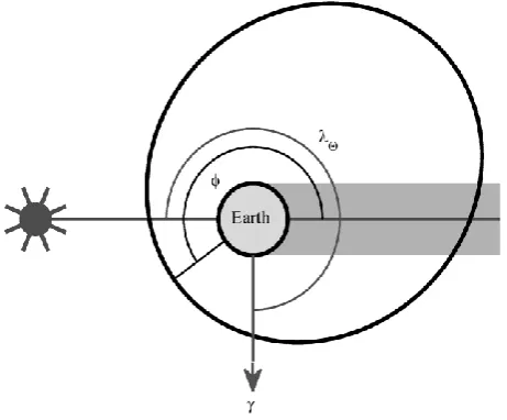
[image:2.595.308.539.344.535.2]The model used in this paper considers an orbit which lies in the ecliptic plane and can be described with three orbital parameters, the semi-major axis a, the eccentricity e and the angle between the Sun-line and the orbit perigee, also defined as the Sun-perigee angle, as shown in Figure 1. When considering the J2 Earth oblateness perturbation the tilt of the Earth‟s axis is neglected to allow an analytical development of the problem.
Figure 1. In-plane orbit geometry.
For an orbit which lies in the ecliptic plane and is only perturbed by solar radiation pressure (SRP) and the J2 perturbation, the dynamics in the e and phase space can be described by the Hamiltonian
2 , SRP J
H as found by
Krivov and Getino [5]:
2
2
, 3
2
( , 1 cos
3 1 )
SRP J
H e e e
e
(1)
3
2
2 7
3 2
3 2
SRP
E
a a n
J R
n a
where n is the orbital rate of the Earth around the Sun and aSRP is the acceleration the spacecraft experiences due to solar radiation pressure. For an Earth-orbiting object with area-to-mass ratio and coefficient of reflectivity cR the
term aSRP can be calculated using the solar energy flux at
Earth F and the speed of light c as follows:
SRP R
F
a c
c
Krivov and Getino [5] divide the parameter space of semi-major axis and area-to-mass ratio into three distinct regions. The behaviors of spacecraft with the area-to-mass ratios investigated in this paper (less than 20 m2/kg) are all within region I for high-altitude orbits (a > 30,000 km). Region I is dominated by solar radiation pressure with the Earth‟s oblateness only having a small effect on the orbital evolution. This means that for the orbits and spacecraft investigated here the J2 perturbation can initially be neglected when devising the control strategy and the Hamiltonian can be reduced to:
2
( , ) 1 cos
SRP
H e e e (2)
This expression was used by Oyama et al. to describe solar sail orbits for geomagnetic tail exploration at apogee distances of 30 Earth radii [7]. The resulting phase space diagram can be divided into three areas. For HSRP 1 it can be shown that the behavior is librational. This means that the orbital eccentricity and perigee angle librate between two values in the form of a loop in the phase space. These orbits have a perigee within 90 degrees of the direction of the Sun, while perigee angle and eccentricity librate around and an equilibrium eccentricity
respectively. For 1 HSRP it can be shown that the behavior is rotational. This means the perigee angle will continually regress while the eccentricity periodically librates. These orbits are most eccentric when the perigee is pointing and least eccentric when the apogee is Sun-pointing. The last area is for orbits with HSRP . These will eventually reach e1 and decay as the orbit perigee intersects the surface of the Earth. To test the premise that for high semi-major axes the J2 perturbation can be neglected a comparison between Eq. (1) and Eq. (2) was performed. The normalized distance between the positions in the phase space calculated with the two different equations was averaged over one loop. Since the time for the completion of a full loop varies for the SRP and J2 case, the positions were not compared at the same time step but rather the same fraction of loop completion. The evolution of orbits with an initially Sun-facing perigee (ϕ = 180 deg) and different starting eccentricities is reported in Figure 2 for four different semi-major axes. In this figure the inaccessible regions are shaded in grey with the critical eccentricity ecrit marked in a dark grey, which represents the
eccentricity at which the perigee equals the Earth‟s radius RE:
1 E
crit
R e
a
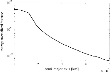
[image:3.595.308.540.206.563.2]It is clear that the two evolutions differ significantly for the 10,000 km orbits but become more similar with increasing semi-major axis. This can also be seen in Figure 3 which shows the average normalized distance between the two orbit evolutions as a function of semi-major axis. For high semi-major axis orbits this is small enough to be neglected.
Figure 2. Evolution of the orbit of a 20 m2/kg spacecraft with c
R = 1.5
in the phase space with SRP and J2 Hamiltonian and SRP only
[image:3.595.306.533.612.758.2]Hamiltonian.
4
B. Equilibrium points in the phase space
In this subsection the areas in the orbital element phase space in which a spacecraft can be stabilized are identified. This is necessary in order to define a goal orbit for orbital control maneuvers. Such maneuvers would seek to navigate SpaceChips towards a long-term stable position.
It can be shown that the secular rate of change of the eccentricity and Sun-perigee angle with respect to the true longitude of the Sun, , in the solar radiation pressure
only case are [5]:
2
2
1 sin
1
cos 1
de
e d
d e
d e
(3)
This is the rate of change of the spacecraft‟s orbital parameters averaged over one orbital revolution around the Earth. It can be seen that the eccentricity has a stable point at {0, } whereas the Sun-perigee angle can only be
kept constant for 3
2 2
. Therefore, a phase space
equilibrium point can only exist at and a fixed
equilibrium eccentricity e0. This equilibrium position was previously identified as stable for the solar sail mission GeoSail [6]:
0
2
1
e
The Hamiltonian has its lowest value of 12 at this phase space equilibrium point.
When considering electrochromic control, instead of a single point, a line of possible stable points emerge which span the two equilibria resulting from different reflectivity values provided by the coating. Here we select two different solar radiation pressure parameters, 1 and
2
corresponding to two different reflectivity states with
1 2
. The condition on eccentricity for a stable controlled equilibrium is then
1 2
2 2
1 2
1 S 1
e
(4)
At these points only the change in eccentricity is zero while the change in Sun-perigee angle with one reflectivity has the opposite sign to that with the other as illustrated in Figure 4. The stabilization at the point PS ( , eS) with eS
defined in Eq. (4) can be achieved with a very simple switching control law for cR,1cR,2:
when
when
R,1
R,2
c c
(5)
Using this strategy a SpaceChip experiences a controlled equilibrium as the derivative of is positive for
0
and negative for 0. This causes the Sun-perigee angle to oscillate closely around and thus the eccentricity to remain constant. This control strategy was first introduced in Ref. [17] which proposed a mission concept employing a SpaceChip swarm for mapping the upper layers of the atmosphere. The orbital parameters are evaluated once per orbital revolution to avoid a jittering control response. Alternatively a dead band could be introduced.
[image:4.595.311.529.319.572.2]Ref. [18] uses an artificial potential field control algorithm in the orbital element phase space to stabilize spacecraft at a greater range of points. It allows a reflectivity change twice per orbit and uses the angles of true anomaly where the switch takes place as control parameters. The resulting area in the phase space in which stabilization is possible includes the range described in Eq. (4). However, the control algorithm is more complex and requires the solution of a two-dimensional optimization problem. This is computationally far more expensive than the algorithm described in Eq. (5) and possibly not suited for SpaceChips with limited computing capabilities.
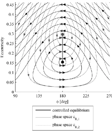
Figure 4. Phase space for a 20 m2/kg spacecraft with two different
reflectivity coefficients cR,1 = 1 and cR,2 = 2 highlighting the region in
which the orbit can be stabilized using the simple switching control law (geo-synchronous orbit used for illustration).
C. Orbit control law
The simple switching control defined in Eq. (5) can stabilize to a point to the orbital element phase space. An equally simple control law for the navigation through the phase space is now sought. In this section it will be shown that a bang-bang control, similar to the time-optimal control of a linear oscillator, can be applied to the problem [19].
This is possible because the solar radiation pressure and J2 Hamiltonian in a polar plot, with coordinate esin and
cos
5 concentric circles around the stable equilibrium position. The superposed phase flow field lines of the orbital evolution with two different values for correspond to the phase space of a linear oscillator with two different centers of oscillation. In both cases the two equilibria lie on an axis with respect to which all phase lines are symmetrical. No phase line can cross another and there are no other equilibria.
Figure 5. Phase space plot (a) and polar plot (b) for a 20 m2/kg
spacecraft on a geosynchronous orbit.
To navigate a spacecraft to any stable point PS identified in Eq. (4), the values of the Hamiltonian at the point with 1 and 2 have to be identified:
2
,1 1
2
,2 2
1
1
S S S
S S S
H e e
H e e
With these values the control law can then be formulated. The desired position can be reached by using
R,1
c when , unless the current orbit is within the loop described by HS,1, and by using cR,2 in when , unless
the correct orbit is within the loop described by HS,2. Figure 6 illustrates this control law as formulated below:
2 ,2
2 ,2
1 ,1
1 ,1
if ( ) ( )
if ( ) ( )
if ( ) ( )
if ( ) ( )
S R,2
S R,1
S R,1
S R,2
H H c
H H c
H H c
H H c
(6)
where H1 is the value of the Hamiltonian with 1 at the
current position and H2 is the value of the Hamiltonian with
2
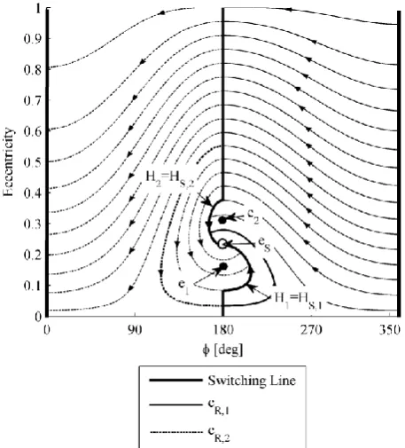
[image:5.595.309.538.293.546.2] at the current position. H1 and H2 change during the maneuver as they depend on the current position, while HS,1 and HS,2 remain constant as they depend on the desired goal position. Figure 6 displays the phase space dynamics when applying the control law formulated above. It can be seen that the desired final position can be reached from all initial positions in the phase space excluding those which would inevitably lead to the eccentricity exceeding unity.
Figure 6. Bang-bang switching law in the phase space to navigate a 20 m2/kg spacecraft on a geosynchronous orbit to the stable position
marked with a black circle.
D. Comparison with a linear oscillator
The proposed switching control algorithm with two fixed reflectivity parameters is the same as the optimal control of a linear oscillator. In the subsection the two are compared to estimate how close the proposed control algorithm comes to be being time optimal.
6 points within the respective area. These regions are highlighted in Figure 7 (in a polar plot). In the case of a linear oscillator the switching solution is always time-optimal even within the highlighted areas because the period of one oscillation is constant and equal for both control options, and the speed along each control path is constant. Therefore in the linear oscillator problem the shortest path connecting two points is always the fastest [19]. The same conditions are not true for the phase space control we consider here. In this section we investigate how close the phase space control comes to fulfilling the two conditions, in other words, (1) how far from equal are the phase space periods with two different reflectivity coefficients, and (2) how far from constant is the speed in the phase space. These two conditions will de addressed in the following paragraph. We refer to „phase space period‟ as the period to cover one complete loop in the phase space; this is far longer than the period for completing one single orbit around the Earth.
Figure 7. Switching law with areas in which proof of time-optimal control is not trivial highlighted.
First the condition on the period of the phase space evolution is investigated. For time-optimality it is required that the period is the same for both values of reflectivity and regardless of the starting position. Oyama et al. [7] find an expression for the period of time T to follow a closed phase path in the case of SRP only:
2
2
1 T
n
This means that for a given area-to-mass ratio, semi-major axis and reflectivity the period to complete one phase space period is constant and not dependent on the starting orbit. However, higher SpaceChips complete one period around a closed phase curve faster. The difference is small: a 10 m2/kg geosynchronous spacecraft would only be 1.8% faster with cR 2than with cR 1. A 20 m
2
/kg spacecraft could increase its libration period by just 6.8%.
The second condition to investigate is how much the rate of orbit evolution in the polar plot deviates from the
average. An analytic formula for the speed of progression along the phase curves can be found as shown in Appendix A:
2
2 2 21 2 1 cos
v e e e (7)
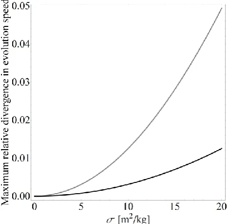
This equation can be numerically evaluated to find the average, the minimum and the maximum speed over one evolution period (i.e. one loop in the phase space) for a given initial orbit and spacecraft characteristics. Using this information the maximum relative divergence from the average speed can be found as a function of area-to-mass ratio and reflectivity. Figure 8 shows the results of this analysis. It depicts the maximum relative difference,
maxv v avg vavg, between actual and average speed of progression along any phase curve for different area-to-mass ratio spacecraft with coefficients of reflectivity of 1 or 2. It can be seen that a 10 m2/kg spacecraft will never diverge more than 1.5% from the average progression speed and a 20 m2/kg spacecraft stays within 5%.
[image:6.595.306.540.372.601.2]It can be seen that for both conditions for the deviation from time optimality is not great with the parameters used in the proposed phase space control. It can therefore be assumed that the resulting maneuver times are approaching the optimum.
Figure 8. Maximum divergence from average progression speed normalized relative to the average along polar phase lines for geosynchronous spacecraft with reflectivity of 1 (black) and 2 (gray).
Modifications to the Hamiltonian model
A. Effect of eclipses on the orbital evolution7 semi-major axis. The precession of the semi-major axis is positive for 0 π, negative for π 2π and zero if
{0, π}
. The effect is such that a spacecraft will return to the semi-major axis orientation it started from after the completion of a full period in the phase space during which the semi-major axis precesses as shown in Ref. [8]. Both effects are small at the distances considered in this paper but are still problematic. The change in semi-major axis during the period further shifts the equilibrium point as e0
is a function of which in turn is dependent on the semi-major axis. With decreasing semi-semi-major axis the eccentricity of the equilibrium point will also decrease. Furthermore additional perturbations act on the spacecraft. Atchison and Peck show that in the case of SpaceChips with area-to-mass ratios in the order of 10 m2/kg and in high altitude orbits the strongest of these effects is the J2 precession already discussed in section 0.A [2].
Although small, the effects of neglecting eclipses and additional perturbations can increase the transfer time considerably because they can lead to the spacecraft missing its target equilibrium point and having to complete another period until it reaches the goal. Since the period of evolution along a closed phase curve is the same regardless of the size of the loop (when only SRP is considered) this can lead to a doubling of transfer time. One solution is to add a margin to the control algorithm that is linearly proportional to the difference between actual and desired eccentricity. This way, a spacecraft would switch its reflectivity too soon rather than too late. Although not ideal, this is far less time consuming.
B. Linearized phase space equations to account for eclipses
In this and the following subsection approaches are discussed to account for the effects of eclipses. The phase space perturbed by the effect of eclipses can be approximated by a linearization process. The original Hamiltonian is linearized around the equilibrium condition in a Cartesian coordinate system based on the polar plot. The linearized equations are then modified to account for a shift in the centre of rotation away from the equilibrium point. The expression for the rotational centre is a function of position and the true equilibrium point location. The effect of eclipses can then be approximated by substituting the analytical equilibrium eccentricity e0 with the real equilibrium which is found numerically taking into account eclipses.
First, the polar coordinates ( , )e are transformed into a
set of auxiliary Cartesian coordinates ( , )x y .
2 2
cos
sin arctan
x e e x y
y
y e
x
(8)
The derivatives of the Cartesian coordinates are (with Eq. (3)):
2
sin
1 cos
x e
y e e
Inserting Eq. (8) delivers:
2 2
1
x y
y x y x
(9)
Linearizing Eq. (9) around the equilibrium point ( , )e0
then defines Cartesian coordinates ( , )x yˆ ˆ for any initial
radial distance r along the x-direction ( 0 ):
0
2
ˆ( ) cos
ˆ( ) 1 sin
x e r
y r
(10)
It can be seen that the radial distance in the y-direction
is 2
1
r . The linearization Eq. (10) assumes a static centre of rotation, e0. We introduce a hypothetical point
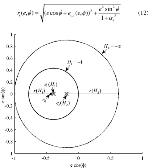
with and eec, the central eccentricity which has equal distance to the maximum and minimum eccentricity within one loop in the phase space. It is equal to the equilibrium eccentricity at the equilibrium point, but decreases with distance from e0. Figure 9 shows the position of ec and r in the polar plot for two different phase lines. The central eccentricity ec can be found as a function
of an initial set of orbital parameters ( , )e by solving Eq. (2) for e with :
, 0
2
( , )
( , ) ( 1, 2)
1
c i
i
H e
e e e i
(11)
where the index i indicates the control mode. i1 corresponds to cR,1 and i2 to cR,2. Next the radius of rotation in the x-direction can be calculated:
2 2
2
, 2
sin
( , ) ( cos ( , ))
1
i c i
i
e
r e e e e
[image:7.595.308.545.472.740.2] (12)
Figure 9. Position of the central eccentricities ec and radial distances in
8 When using two different coefficients of reflectivity any set of orbital coordinates can be transformed into radial coordinates which are unique within one half of the phase space ((0, ) ( , 2 )) . The coordinates are ( , )r r1 2
and correspond to the radial distance in the x-direction with cR,1 and cR,2. Using Eqs. (11) and (12), Eq. (10) can be revised to:
,
2
ˆ ( ) cos
ˆ ( ) 1 sin
i c i i
i i i
x e r
y r
(13)
By substituting the analytical result for the equilibrium point e0 with a numerical solution e0,ecl which takes into account the eclipses when computing ec i, in Eq. (11), the linearization Eq. (13) becomes an accurate approximation of the perturbed phase space resulting from the compensation for eclipses. Although the real equilibrium
0,ecl
e is close to the analytical equilibrium e0, this step is necessary because maneuvers in the vicinity of the equilibrium are sensitive to the exact position. If an incorrect value for the equilibrium eccentricity is assumed the control algorithm could in certain cases fail to complete the maneuver. To find e0,ecl, the equation for the secular change in found by Colombo and McInnes [8] is
calculated for orbits with and the eccentricity e0,ecl is found numerically for which this equation equals zero (see Appendix B).
Figure 10 shows the results of the linearization superimposed on those of a numerical simulation with eclipses. For the dynamical equations which consider eclipses, used here for computing the numerical results the reader can refer to Eqs. (5)-(11) by Colombo and McInnes [8]. It can be seen that the linearized phase lines in Figure 10 (b) match the numerical results far better than the Hamiltonian phase lines in Figure 10 (b).
Using this approach the control algorithm in Eq. (6) can be revised to:
2 2,
2 2,
1 2,
1 2,
if ( ) ( )
if ( ) ( )
if ( ) ( )
if ( ) ( )
S R,2
S R,1
S R,1
S R,2
r r c
r r c
r r c
r r c
where ( , )r r1 2 are the radial coordinates of the current
orbit as described above and (r1,S,r2,S) are the radial coordinates of the desired stable goal point.
C. Control algorithm for constant semi-major axis
The method described in the previous subsection can account for the inaccuracies caused by the effect of eclipses to allow more precision in the selection of the control path. However, it does not remove all effects of eclipses and the spacecraft arrive at the correct position in the ( , )e phase
space, but with a different semi-major axis. In this subsection it is shown how the electrochromic properties of the spacecraft can be used to keep the semi-major axis
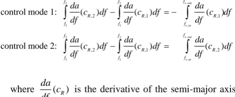
constant as well as efficiently navigating the spacecraft through the phase space. To achieve this, the reflectivity has to be switched twice per orbit. That way there are always two possible control modes. One in which the reflectivity is predominantly high, control mode 1, and one in which the reflectivity is predominantly low, control mode 2. The switching angles, f1 and f2 have to fulfill the
following expression in which fe in, and fe out, represent the angles of true anomaly at which the eclipse is entered and exited given by Eqs. (7)-(9) in Ref. [8]:
,
2 2
1 1 ,
,
2 2
1 1 ,
, 2 ,1 ,1
, 2 ,1 , 2
control mode 1: ( ) ( ) ( )
control mode 2: ( ) ( ) ( )
e out
e in
e out
e in
f
f f
R R R
f f f
f
f f
R R R
f f f
da da da
c df c df c df
df df df
da da da
c df c df c df
df df df
where ( R) da
c
df is the derivative of the semi-major axis
[image:8.595.309.545.193.290.2]with respect to the true anomaly due to solar radiation pressure for the given reflectivity.
Figure 10. Comparison between phase space with eclipses and Hamiltonian phase space (a) and approximating linearization (b) for a spacecraft with σ = 20 m2/kg and c
[image:8.595.318.539.324.745.2]9 The interval of the eclipses and the interval of reflectivity change [ ,f f1 2] may not overlap. To find close to optimal switching angles with as little computational expense as possible we reduce the parameter from two to one dimensions. Instead of searching for both switching angles as proposed in [18], [ ,f f1 2] is redefined as
[fc f f, c f] where fc is the angle in the centre of the
interval and f f1fc f2fc determines the size of
the interval. Of these two variables only fc needs to be
found numerically, f is found analytically by a linear approximation.
First fc is determined. For the maneuver to be most effective means the interval is to be as small as possible so that the orbit evolution will follow closely the behavior predicted by the Hamiltonian. To achieve this fc is chosen as the angle at which the positive or negative change of semi-major axis over true anomaly is greatest. Whether the direction of the change is negative or positive depends on the control mode and the change in semi-major axis which would occur without control, a.
control mode 1:
0
2
control mode 2:
0
2
c min
c max
c max
c min
f f
f f
f f
f f
where fmax is the true anomaly where the greatest positive rate of change of semi-major axis over true anomaly occurs, and fmin is the angle of true anomaly where the greatest negative change occurs. The change of semi-major axis is positive when the velocity vector of the spacecraft is pointing away from the Sun and negative if it is pointing towards it. The angles at which it is maximal and minimal can be found by maximizing or minimizing the following equation which has been derived by combining the Gauss‟ equation for variation of semi-major axis [20] with the orbit geometry to deduce the direction of solar radiation pressure, so that the rate of change of semi-major axis scales as:
sin(2 ) sin( )
da
e f f
df
Next f , the size of the interval in true anomaly to
each side of the central angle fc, is determined. It is found by linear approximation:
,
, ,
,
,1 , 2 ,1
, 2 , 2 ,1
control mode 1:
control mode 2:
( )
( ) ( )
2 ( ) ( )
( )
( ) ( )
2 ( ) ( )
e out
e in
e out
e in
f R
c c
R R
f
f R
c c
R R
f da c
da f da f
f c c df
df df df
da c
da f da f
f c c df
df df df
(14)
where the right hand term is the change in semi-major axis which would occur due to eclipses over one orbit if the reflectivity is constant. The integral does not have to be
calculated numerically. Instead the analytical expressions in Ref. [8] are used (see Appendix C). The left term corresponds to the difference in change of semi-major axis caused by using the other reflectivity. This is assuming a constant rate of change of semi-major axis over that interval. This assumption can be made because the interval is small. A comparison with the exact results for the required f obtained using a numerical simulation was conducted and it was found that at geosynchronous semi-major axis and eccentricities below 0.5 this simplification is appropriate. At higher eccentricities a numerical approach can be used to find f using the value calculated in Eq. (14) as an initial guess.
Using this method we can account for eclipses with comparatively low computational expense as all but one step in the control algorithm are analytical and the numerical step is a simple one-dimensional optimization. Since a linear approximation is used to determine f , and
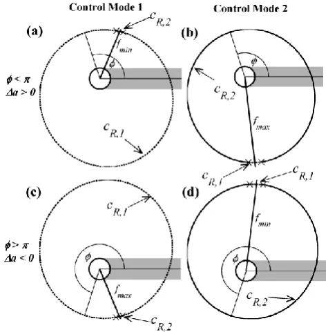
[image:9.595.317.555.450.691.2]because we are neglecting any out-of-plane dynamics, there will still be a change in semi-major axis. However, it is expected that this change is small in comparison to using the method in which the reflectivity is switched only depending on the position in the phase space as described in the previous sections. Figure 11 shows the results for the two control modes for a geosynchronous orbit with an eccentricity of 0.3 and two different initial perigee angles. For eccentricities below 0.5 at geosynchronous semi-major axis f 2.5. This causes the evolution of the orbital elements to follow closely the evolution with eclipses and the linearized approach to the control algorithm described in the previous section can be used.
Figure 11. Switching law in control mode 1 and 2 for two example orbits. The arc of the orbit with cR,1 is drawn in solid and cR,2 in
dashed. The positions at which the reflectivity is switched are marked with crosses. Figures (a) and (b) show the control strategy when the change in semi-major axis over one orbit would be positive and (c) and (d) show the control strategy when the change in semi-major axis would be negative. The left column of figures shows the control strategy with mainly reflectivity cR,1 and the right column shows the
10
Results
A. Test case maneuver
To show the effectiveness of the proposed control methods a test case was devised and simulated. The mission scenario consists of six SpaceChips with an area-to-mass ratio of 15 m2/kg which are initially in six different orbits with a semi-major axis of 42,000 km, eccentricity ranging from close to circular to under 0.5 and perigee angle between 90 and 270 degrees. They are to be collected into a stable goal orbit with eS 0.25 and = 180°. The maneuver is performed using the using the linearized phase space introduced in section 0.B the maneuvers were performed with and without the constant semi-major axis control derived in section IV.C. The orbit was propagated numerically taking solar radiation pressure and the Earth oblateness into account, while the control algorithms use the linearized phase space introduced in section 0.B. The numerical propagation is performed using the Gauss‟ equations in true anomaly and taking out-of-plane dynamics into account. When using a full set of Keplerian orbital parameters, the angle can be calculated as follows:
( )
where is the right ascension of the ascending node and the argument of perigee. The control algorithm uses the computationally inexpensive linearized phase space model. It is assumed that the spacecraft receive accurate information about their current state, eccentricity and , once every orbit and then decide on the control mode using the algorithm detailed in this paper. This way it can be shown that the control method is also robust towards perturbations which have not been taken into account in the control algorithm such as eclipses, the J2 effect and out-of plane dynamics.
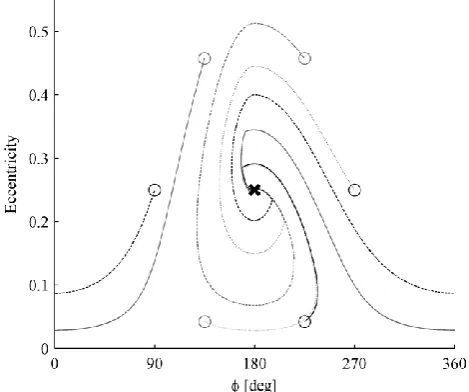
[image:10.595.305.540.56.252.2]The control algorithm accomplished the objective to assemble all six spacecraft at the desired eccentricity and orbit orientation. This was achieved in less than 1.3 years. However, the SpaceChips in the study which did not use the constant semi-major axis control ended up at different semi-major axes of between 41,000 km and 43,000 km. This can be avoided using the computationally more expensive (i.e., the reflectivity coefficient is changed twice per orbit) constant semi-major axis control. The evolution in the phase space in the latter case is shown in Figure 12. The evolution of all orbital parameters over the course of the maneuver is shown in Figure 13. In this case the semi-major axis only varies on the order of 100 km. The cause for this small variation is the change in inclination which changes the actual eclipse angles in 3D geometry from the ones calculated analytically in the plane within the control loop. Figure 14 visualizes the evolution of the orbits during the maneuver.
Figure 12. Maneuvers of six SpaceChips with σ = 15 m2/kg toward the
same orbit in the phase space using the control algorithm described in section IV.C.
Figure 13. Evolution of orbital parameters during the maneuvers of six SpaceChips with σ = 15 m2/kg toward the same orbit in the phase
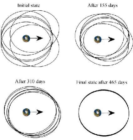
[image:10.595.311.527.324.736.2]11 Figure 14: Evolution of the orbits of the six spacecraft during the
maneuver as a projection onto the ecliptic plane in a Sun-following reference frame. The arrow indicates the direction of the solar radiation.
B. Long-term stability
[image:11.595.312.536.259.517.2]In Figure 13, it can be seen that the right ascension of the ascending node and the inclination are decreasing over the course of the maneuver. Although the change is small enough not to affect the accuracy of the controller, questions about the long-term stability of the goal orbit may be raised. A SpaceChip of the same specifications as those used in the maneuver simulation and using the linearized phase space control algorithm was propagated for fifty years at the goal orbit. The results of this simulation can be seen in Figure 15.
Figure 15. Long-term evolution of a controlled spacecraft at an artificially stable orbit.
It can be seen that the controlled parameters e and remain close to their initial value while the other orbital parameters oscillate within bounds. It can be concluded that a SpaceChip at geosynchronous altitude can be stabilized in the long term using the proposed control algorithm.
C. Maneuver time
Figure 16 shows the time until the completion of a maneuver using the linearized phase space control algorithm without controlling the semi-major axis starting from different points in the phase space. The hatched areas indicate the position from which a maneuver is impossible because impact with the Earth is inevitable (eecrit). The stable eccentricity can be reached from any position within three years.
Figure 16. Time until reaching goal orbit marked with x from different positions in the phase space (a = 42,000 km) using the linearized phase space control for a SpaceChips with = 15 m2/kg.
Conclusions
[image:11.595.49.273.501.746.2]12 with a differential equation solver considering solar radiation pressure and the Earth‟s oblateness. The scenario results show that the closed feedback control algorithm can cope with other minor perturbing effects at high semi-major axis. It was also shown that the goal orbit is long-term stable. The control presented in this paper can also be applied to other mission scenarios. For example it can be envisaged that a group of SpaceChips is released in a common orbit, from where they spread out into different orbits using electrochromic control. In this scenario a reverse maneuver to the one needed to collect the spacecraft would be performed.
Appendix
A. Derivation of the speed of evolution along the phase lines in the Cartesian coordinates
This section of the appendix contains the calculations needed to derive Eq. (7) in Section 0.D. In order to find the speed of orbital evolution in polar coordinates for a given initial condition, a coordinate transformation has to be performed from ( , )e to ( , ) . The latter is a polar
coordinate system with the centre at the equilibrium point for a given , as shown in Figure 17. The following expressions are found which define the transformation:
2 2
2 2
( , ) 2 cos
1 1
e
(15)
2
cos 1 ( , ) arccos
( , ) e 0 cos cos
e e (16)
An expression for as a function of , H and is found by inserting Eq. (15) and Eq. (16) into Eq. (2) and then solving for so that
2 2 2 2 2 2 2 2 2 2 21 1 cos
, ,
1 cos
1
1 1 1 cos 2
1 1 1 cos H H H H
Defining
e e0
as the difference between theeccentricity at and the equilibrium eccentricity gives
the value of the Hamiltonian as a function of :
2
2 2
, 1
1 1
H
Next the speed of progression along the phase curves in the polar plot ( , )x y ( cos , sin )e e is derived using:
2
22 2
cos sin sin cos
v x y e e e e
and with Eq. (3) this reduces to:
22 2
, sin 1 cos
v e e ee
From Eq. (19) the following equation can be derived in the transformed polar coordinates system:
2
2 2 2( , ) 1 ( , ) 2 ( , ) 1 ( , ) cos ( , )
v e e e
[image:12.595.311.540.265.465.2]This expression was then analyzed to provide the data shown in Figure 8.
Figure 17. Coordinate transformation to equilibrium centered coordinates.
B. Calculation of the equilibrium eccentricity with eclipses
This section of the appendix contains the equation used in the numerical calculation of e0,ecl, the equilibrium
eccentricity when considering in-plane orbits with eclipses in Section 0.B.
, , 2 0, 0 3
0, , 0, , 3
( , ) d d 0
fun ( , ) fun ( , ) 2 0
e in
e out
f
ecl f
ecl e in ecl e out
d d
e f f
df df
a
e f e f
a
13 radiation pressure found by Colombo and McInnes [8] the indefinite integral for , fun, can be defined analytically:
2 2 2 3 2 2 2 2
2 2 2
(1 ) 3 1
fun ( , ) arctan tan
1 2
1
cos sin
(1 ) sin 1
2
(1 )(1 cos ) (1 )(1 cos )
SRP
SRP
a e e f
e f a
e e e
e f f
a e e f
a
e e e f e e f
C. Analytical formula for the derivative of semi-major axis with respect to true anomaly
This section of the appendix contains the equation used in the analytical calculation of the change in semi-major axis over an arc of true anomaly used in the control algorithm in Section 0.C.
2
1
2 1
( , , ) d fun ( , , , ) fun ( , , , )
f
a a
f
da
a e f a e f a e f
df
Using the equations for the change in orbital elements due to solar radiation pressure found by Colombo and McInnes [8] the indefinite integral for a, funa, can be
defined analytically:
3 2
2 (1 ) cos sin sin
fun ( , , , )
(1 cos )
a SRP
a e e f
a e f a
e e f
Acknowledgments
This work was funded by the European Research Council project VISIONSPACE (227571). Charlotte Lücking is also supported by the IET Hudswell International Research Scholarship and the Frank J. Redd Student Scholarship.
References
[1] Hamilton, D. P., and Krivov, A. V. "Circumplanetary Dust Dynamics: Effects of Solar Gravity, Radiation Pressure, Planetary Oblateness, and Electromagnetism," Icarus Vol. 123, No. 2, 1996, pp. 503-523.
doi: 10.1006/icar.1996.0175
[2] Atchison, J. A., and Peck, M. "Length Scaling in Spacecraft Dynamics," Journal of Guidance, Control, and Dynamics Vol. 34, No. 1, 2011, pp. 231-246.
doi: 10.2514/1.49383
[3] Jakes, J. W. C. "Project Echo." Vol. 39, Bell Laboratories, New York, NY, United States, 1961, pp. 306-311.
[4] Shapiro, I. I., and Jones, H. M. "Perturbations of the Orbit of the Echo Balloon," Science Vol. 132, No. 3438, 1960, pp. 1484-1486. doi: 10.1126/science.132.3438.1484
[5] Krivov, A. V., and Getino, J. "Orbital evolution of high-altitude balloon satellites," Astronomy and Astrophysics Vol. 318, 1997, pp. 308-314.
[6] McInnes, C. R., Macdonald, M., Angelopolous, V., and Alexander, D. "GEOSAIL: Exploring the geomagnetic tail using a small solar sail," Journal of Spacecraft and Rockets Vol. 38, No. 4, 2001, pp. 622-629.
doi: 10.2514/2.3727
[7] Oyama, T., Yamakawa, H., and Omura, Y. "Orbital dynamics of solar sails for geomagnetic tail exploration," Journal of Guidance, Control and Dynamics Vol. 45, No. 2, 2008, pp. 316-323.
doi: 10.2514/1.31274
[8] Colombo, C., and McInnes, C. R. "Orbital dynamics of „smart dust‟ devices with solar radiation pressure and drag," Journal of Guidance, Control and Dynamics Vol. 34, No. 6, 2011, pp. 1613-1631.
doi: 10.2514/1.52140
[9] Warneke, B., Last, M., Liebowitz, B., and Pister, K. S. J. "Smart Dust: communicating with a cubic-millimeter computer," Computer Vol. 34, No. 1, 2001, pp. 44-51.
doi: 10.1109/2.963443
[10] Barnhart, D. J., Vladimirova, T., and Sweeting, M. N. "Very-small-satellite design for distributed space missions," Journal of Spacecraft and Rockets Vol. 44, No. 6, 2007, pp. 1294-1306. doi: 10.2514/1.28678
[11] Atchison, J. A., and Peck, M. A. "A passive, sun-pointing, millimeter-scale solar sail," Acta Astronautica Vol. 67, No. 1-2, 2009, pp. 108-121.
doi: 10.1016/j.actaastro.2009.12.008
[12] Atchison, J. A., and Peck, M. "A millimeter-scale lorentz-propelled spacecraft," Proceedings of the AIAA Guidance, Navigation, and Control Conference; Vol. 5, Hilton Head, SC, United states, 2007, pp. 5041-5063.
[13] Schaub, H., Parker, G. G., and King, L. B. "Challenges and prospects of Coulomb spacecraft formation control," Proceedings of the John L.Junkins Astrodynamics Symposium; Vol. 52, 2004, pp. 169-193.
[14] Kawaguchi, J., Mimasu, Y., Mori, O., Funase, R., Yamamoto, T., and Tsuda, Y. "IKAROS - Ready for lift-off as the world's first solar sail demonstration in interplanetary space," 60th International
Astronautical Congress. Daejeon, Korea, 2009.
[15] Demiryont, H., and Moorehead, D. "Electrochromic emissivity modulator for spacecraft thermal management," Solar Energy Materials and Solar Cells Vol. 93, No. 12, 2009, pp. 2075-2078. doi: 10.1016/j.solmat.2009.02.025
[16] De Juan Ovelar, M., Llorens, J. M., Yam, C. H., and Izzo, D. "Transport of Nanoparticles in the Interplanetary Medium," 60th
International Astronautical Congress. Daejeon, Republic of Korea, 2009.
[17] Colombo, C., Lücking, C. M., and McInnes, C. R. "Orbit evolution, maintenance and disposal of SpaceChip swarms," 6th International Workshop on Satellite Constellation and Formation Flying (IWSCFF 2010). Taipei, Taiwan, 2010.
[18] Lücking, C., Colombo, C., and McInnes, C. R. "Orbit Control of High Area-to-Mass Ratio Spacecraft using Electrochromic Coating," 61st International Astronautical Congress. IAF, Prague,
Czech Republic, 2010.
[19] King, A. C., Billingham, J., and Otto, S. R., “Time-Optimal Control in the Phase Plane,” Differential Equations: linear, nonlinear, ordinary, partial, 1st ed., Cambridge University Press, United Kingdom, 2003, pp. 417-446.
[20] Stark, J. P. W., Swinerd, G. and Fortescue, P. W., “Celestial Mechanics,” Spacecraft System Engineering, 3rd ed., Wiley,