Singular spectrum analysis for identifying structural nonlinearity using free-decay responses : Application detection and diagnosis in composite laminates

(1)

Singular Spectrum Analysis for identifying structural

nonlinearity using free-decay responses. Application for

delamination detection and diagnosis in composite

laminates.

D. Garcia1, I. Trendafilova1

1_{University of Strathclyde, Department of Mechanical and Aerospace Engineering}

75 Montrose street, Glasgow G1 1XJ, United Kingdom e-mail: [email protected]

Abstract

This investigation considers a methodology for analysis of the vibratory response of composite laminate structures which is based on Singular Spectrum Analysis. Composite laminate structures generally demon-strate nonlinear dynamic behaviour as a result of their intrinsic material nonlinear nature. Since the nonlin-earities on a number of occasions induce relativity small changes in the vibratory response which are difficult to identify, the raw measured dynamic responses have to be subjected to certain pre-treatment before it can be used for purposes of nonlinearity and damage analysis. To approach this problem this work investigates the effect of some key signal and transformation parameters, such as signal length and sampling frequency as well as the SSA window length on the performance of the methodology itself. The selection of these parameters has a direct influence on the damage sensitivity and the accuracy of the methodology. The vari-ation of these parameters can produce radical changes on the clustering effect of the methodology and it is demonstrated that this might affect the results interpretation.

1 Introduction

The growth of the engineering challenges in different industry sectors requires the development of proper Structural Health Monitoring (SHM) methodologies to inspect the integrity and the health of structures. The rapid developments in this area are due to the real engineering problems related to safe design, manufac-turing, maintenance and safe operation of the technical infrastructure. A similar way, introduction of new materials for engineering infrastructures gives an additional importance to SHM. In particular the use of composite materials is growing as they are continuously replacing traditional ones. Composites are gener-ally implemented in structures with high performance requirements and their nature depends on the material composition. The interaction between their components makes their analysis still more difficult. The differ-ent properties of their compondiffer-ents generate interface failures that often result delamination. Delamination in composite structures affects adversely the system’s performance while in the same time they can lose up to 60% of their stiffness and still remain visibly unchanged. Accordingly the development of proper SHM methodologies becomes a must for such materials and structures.

(2)

methods do not assume any model or linearity and they are purely based on the measured structural vibratory response. The methods developed and being developed for composite structures are primarily non-model based one due to the fact such materials are difficult to model precisely. In practice most of the purely data-driven methodologies make use of data analysis and utilize different statistical methods and characteristics to extract features which characterize the health and integrity of a structure [1]. In this paper a method based on Singular Spectrum Analysis (SSA) is introduced. SSA is a technique applied for time series analysis which incorporates multivariate analysis, dynamical systems analysis and signal processing [2]. SSA uses Principal Component Analysis [3, 4] as a technique for the analysis of auto-correlated non-independent time series [?]. SSA is applied for diverse applications ranging mathematics and physics [6] to weather forecasting [7], financial mathematics [8], market research and social sciences [9]. The aim of SSA is to decompose the original signal using a small number of independent and much more interpretable components which can be used for trend identification, detection of oscillatory components, periodicity extraction, signal smoothing, noise reduction and detection of structural changes in time series [2].

SSA is applied in this study to develop a methodology for damage and delamination assessment in composite laminate structures. The developed methodology is able to detect structure changes in the vibratory response of the composite laminated structures. In general, damage and delamination introduce small differences in the vibratory response of the structure which are difficult to detect and process for the purposes of damage assessment. Differently from traditional spectrum analysis, SSA is able to uncover rotational periodicities at any frequency. Thus, in a certain sense it can be applied for the purpose of modal analysis for non-linearly vibrating structures. In this paper, a method based on SSA decomposition was developed to address the problem for delamintaion assessment in composite structures [10]. SSA is highly sensitive to changes in a dynamical system therefore it can be used as a powerful tool for nonlinearities detection including damage and/or delamination. However, this sensitivity is highly dependant on the choice of the signal parameters. Significant changes in the time series structure can be detected for any reasonable choice of parameters [11]. To detect small changes in noisy series careful tuning of some of the key parameters is required. To approach this problem this work investigates the effect of some key signal and transformation parameters, such as signal length and sampling interval as well as the window length on the precision and the performance of the methodology. The proper selection of these parameters is demonstrated to have direct influence on the sensitivity to damage and the accuracy of the methodology. The variation of these parameters can produce radical changes on the clustering effect of the methodology and it might affect the results interpretation. This study approaches the above mentioned problems for two cases: a simple nonlinear 2-DoF spring-damper-mass system and for a real experiment performed for composite laminate beams.

The paper is organized as follows.

At §2, the delamination assessment methodology is detailed. Firstly a short description of the steps fol-lowed by the suggested SSA based in the methodology is described and secondly its application for damage assessment is introduced.

§3 is devoted to the study of some signal and another parameters and how they can affect the results and the performance of the methodology. The methodology is applied for the 2-DoF system and the effect of the parameters in question is then analyzed.

(3)

2 Damage and delamination assessment methodology

Multiple realisations of the data recorded (accelerations) were arranged into vectors

xi = (xi₁,xi₂, ...,xi_j, ...,xi_N)0 where i = 1,2, ..., M is the number of realisations and j = 1,2, ..., N is the number of components in each signal.

Each signal was transformed into the frequency domain. In this way, the spectral data matrix

Z= (z1,z2, ...,zi, ...,zM)was obtained with all vectors arranged in columns. The next step is to embed the vibratory responses.

Given a window with lengthW (1 < W ≤ N₂), theW−frequency-lagged vectors arranged in columns are used to define the trajectory matrix. These vectors are padded with zeros to keep the same vector length. The embedding matrix Ze is the representation of the system in a succession of overlapping vectors of the time

series by W points.

At the next step, the covariance matrix of the matrixZewas obtained following the Equation 1 bellow, where

N0 = N₂.

CZ =

e Z0Ze

N0 (1)

The eigenvaluesλkand the eigenvectorsρkofCZ were obtained according to the following expression.

CZρk=λkρk (2)

The eigenvaluesλk were then arranged in the diagonal matrixΛΛΛZ in decreasing order and the matrixEZ

contains their corresponding eigenvectorsρkwritten as columns. TheEZ vectors are called Empirical

Or-thogonal Functions (EOFs) and they contain the data as a decomposition into orOr-thogonal basis. The eigen-values define the partial variance of each eigenvectors, therefore the total sum of all of these variances gives the total variance ofZe.

E0_ZCZEZ= ΛΛΛZ (3)

The projection of the measured dataZe onto the matrixE_Z yields the corresponding Principal Components

(PCs) matrixA=ZEe _Z.

A matrix which contains the projection of the PCs onto the new space was created to reconstruct the signal. The Reconstructed Components (RCs) were obtained according to Equation (4). For a given set of indicesK corresponding to a set of PCs, the RCs were obtained by projecting the corresponding PCs onto the EOFs.

Rk_m,n = 1

W

X

w=1

Ak_n₋_wEk_m,w (4)

where k−eigenvectors give the kth RC atn−frequency between n = 1...N0 for each m−channel (m = 1...M) which was embedded inw−lagged vectors (w= 1,2, ..., W).

(4)

The components containing more of the variance of the initial signal contain more information about the signal itself. Therefore, these RC’s are expected to contain most of the information about the vibratory system and the changes in it.

3 Some parameters and their effect on the method

3.1 The2−DoFsystem

As was mentioned, the above methodology is first applied to 2-DoF system defined by the Equation 5.

[M]¨x+ [C] ˙x+ [K]x+f( ˙x,x) = 0 (5)

where[M],[C],[K]are constant coefficients mass, damping and stiffness matrices respectively defined by the Equation (6). The functionf( ˙x,x) provides a quadratic coupling between masses and it is defined by Equation (7).

[M] =

m1 0

0 m2

[C] =

c1+c2 −c2 −c2 c2+c3

[K] =

k1+k2 −k2 −k2 k2+k3

(6)

f( ˙x,x) =

−kn(x2+x1)2

kn(x2+x1)2

(7)

The following initial conditions and parameter values used x(1)₀ = x(2)₀ = 0 m, x˙(1)₀ = 0m/s2_, _x_˙(2)

0 =

1m/s2,k1 =k2 =k3 = 2000N/m,kn= 10000N/m,c1 =c2 =c3 = 6N m/sandm1 =m2 = 5kg.

These values correspond to the baseline healthy state of the system. An initial velocity was applied tom2to simulate an impulse. The system describes a free-decay response and the acceleration was recorded by each instant of time to generate the data to introduce in the methodology.

Damage was introduced in the 2-DoF system by introducing different levels of stiffness reduction which simulate different damage levels. Reduction of10%,20%and30%are applied to the nonlinear stiffnesskn.

Multiple realizations were generated by the introduction of white noise at20dBto the obtained accelerations. The system is used as a model to analyze the effect of the parameters in the accuracy of the method described in§2. The accuracy of the method is judged by the detection of the stiffness reduction inkn. In the next two

sections the effect of signal length, the sampling frequency interval (∆f) and the window length (W) are studied and analyzed.

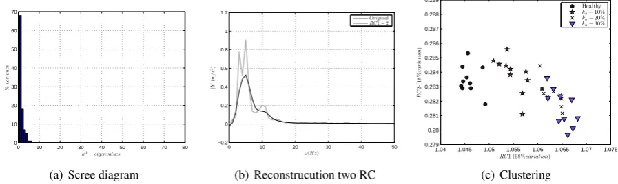
3.2 Effect of the sampling frequency and the signal length

The following paragraphs discuss the principal considerations for selecting the sampling frequency interval

∆f and the signal length for a successful delamination detection.

(5)

0 10 20 30 40 50 60 70 80 0 10 20 30 40 50 60 70

kth−eigenvalues

% v a r ia nc e

(a) Scree diagram

0 10 20 30 40 50

−0.1 0 0.1 0.2 0.3 0.4 0.5 0.6 0.7 0.8 0.9 | Y | ( m / s 2)

ω(Hz)

Original

RC1−2

(b) Reconstrucution two RC

1.335 1.34 1.345 1.35 1.355 1.36

0.232 0.234 0.236 0.238 0.24 0.242 0.244

RC1-(67%variation)

R C 2 -( 1 2 % v a r ia ti o n ) Healthy

kn−10%

kn−20%

kn−30%

[image:5.595.80.528.86.222.2]

(c) Clustering

Figure 1: For a fixedW = 7the effects on the variation of sampling frequency. The resolution of the signal was recorded2.56slong and sampled at400Hz. For the visualization issue, theωscale was reduced until

50Hz.

0 10 20 30 40 50 60 70 80

kth−eigenvalues

% v a r ia nc e

(a) Scree diagram

0 10 20 30 40 50

−0.1 0 0.1 0.2 0.3 0.4 0.5 0.6 0.7 | Y | ( m / s 2) ω(Hz) Original

RC1−2

1.408 1.41 1.412 1.414 1.416 1.418 1.42 1.422 1.424 1.426

0.265 0.27 0.275 0.28 0.285 0.29

RC1-(71%variation)

kn−10%

kn−20%

kn−30%

[image:5.595.81.525.287.422.2]

(c) Clustering

Figure 2: For a fixedW = 7the effects on the variation of sampling frequency. The resolution of the signal was recorded 2 slong and sampled at400Hz For the visualization issue, the ω scale was reduced until

50Hz.

0 10 20 30 40 50 60 70 80

0 10 20 30 40 50 60 70

kth−eigenvalues

% v a r ia nc e

(a) Scree diagram

0 10 20 30 40 50

−0.2 0 0.2 0.4 0.6 0.8 1 1.2 | Y | ( m / s 2)

ω(Hz)

Original

RC1−2

1.04 1.045 1.05 1.055 1.06 1.065 1.07 1.075

0.279 0.28 0.281 0.282 0.283 0.284 0.285 0.286 0.287 0.288 0.289

RC1-(68%variation)

kn−10%

kn−20%

kn−30%

(c) Clustering

Figure 3: For a fixedW = 7the effects on the variation of sampling frequency. The resolution of the signal was recorded1slong and sampled at400Hz. For the visualization issue, theω scale was reduced until

50Hz.

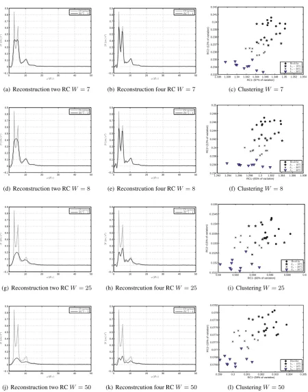
3.3 Effect of the window lengthW

The following paragraphs discuss the principal considerations for selecting the window length W for a successful delamination detection.

[image:5.595.77.526.485.619.2]

(6)

0 10 20 30 40 50 −0.1 0 0.1 0.2 0.3 0.4 0.5 0.6 0.7 0.8 0.9 | Y | ( m / s 2)

ω(H z)

Or iginal

RC1−2

(a) Reconstruction two RCW = 7

0 10 20 30 40 50

−0.1 0 0.1 0.2 0.3 0.4 0.5 0.6 0.7 0.8 0.9 | Y | ( m / s 2)

ω(H z)

Or iginal

RC1−4

(b) Reconstruction four RCW = 7

1.336 1.338 1.34 1.342 1.344 1.346 1.348 1.35 1.352 1.354 0.233 0.234 0.235 0.236 0.237 0.238 0.239 0.24 0.241 0.242

RC1−(67% of variation)

Healthy

kn−10%

kn−20%

kn−30%

(c) ClusteringW= 7

0 10 20 30 40 50

−0.1 0 0.1 0.2 0.3 0.4 0.5 0.6 0.7 0.8 0.9 | Y | ( m / s 2) ω(H z) Or iginal

RC1−2

(d) Reconstruction two RCW = 8

0 10 20 30 40 50

−0.1 0 0.1 0.2 0.3 0.4 0.5 0.6 0.7 0.8 0.9 | Y | ( m / s 2) ω(H z) Or iginal

RC1−4

(e) Reconstrcution four RCW = 8

1.292 1.294 1.296 1.298 1.3 1.302 1.304 1.306 1.308 0.234 0.236 0.238 0.24 0.242 0.244 0.246 0.248 0.25

Healthy

kn−10%

kn−20%

kn−30%

(f) ClusteringW = 8

0 10 20 30 40 50

−0.1 0 0.1 0.2 0.3 0.4 0.5 0.6 0.7 0.8 0.9 | Y | ( m / s 2)

ω(H z)

Or iginal

RC1−2

(g) Reconstruction two RCW = 25

0 10 20 30 40 50

−0.1 0 0.1 0.2 0.3 0.4 0.5 0.6 0.7 0.8 0.9 | Y | ( m / s 2)

ω(H z)

Or iginal

RC1−4

(h) Reconstrcution four RCW = 25

0.59 0.592 0.594 0.596 0.598 0.6

0.1515 0.152 0.1525 0.153 0.1535 0.154 0.1545 0.155

Healthy

kn−10%

kn−20%

kn−30%

(i) ClusteringW = 25

0 10 20 30 40 50

−0.1 0 0.1 0.2 0.3 0.4 0.5 0.6 0.7 0.8 0.9 | Y | ( m / s 2) ω(H z) Or iginal

RC1−2

(j) Reconstruction two RCW = 50

0 10 20 30 40 50

−0.1 0 0.1 0.2 0.3 0.4 0.5 0.6 0.7 0.8 0.9 | Y | ( m / s 2) ω(H z) Or iginal

RC1−4

(k) Reconstrcution four RCW = 50

0.299 0.3 0.301 0.302 0.303 0.304 0.305 0.0766 0.0768 0.077 0.0772 0.0774 0.0776 0.0778 0.078 0.0782

Healthy

kn−10%

kn−20%

kn−30%

[image:6.595.77.528.84.656.2]

(l) ClusteringW = 50

Figure 4: Effects on the variation ofW forW = 7,W = 8,W = 25andW = 50in the analytical model. The resolution of the signal was fixed at2.56slong and sampled at= 400Hz. For the visualization issue, theωscale was reduced until50Hz.

(7)

A general aspect for the selection ofW is that longer window length will provide more detailed decompo-sition. According to this statement, the best detailed decomposition is obtained for W ' N

2. Despite the

previous statement, a large window length will require more components but it can in the same time intro-duces more noise in the reconstruction [13, 14]. In this case, it is worth testing different window lengths starting from large values ofW until the proper effect is achieved.

In order to study the effect on the delamination detection caused by the window length, the signals were recorded for2.56sand sampled at400Hz.

As it is shown in Figure 4, large window length results in a smoother the signal and distributes the information about the dynamical system over more principal components. Then, the first two principal components does not provide a good reconstruction (see Figure 4(g) and Figure4(j)). The delamination assessment is based on the data projection onto the first two principal components as it is described in§2. In the Figure 4 can be observed that the variation ofW alteres the results. For instance, in this particular case, the reconstruction which uses four principal components provides a very good reconstruction of the original signal(see Figure 4(b) and Figure 4(e)).

Large values ofW does not provide good results in the clustering effect as it is shown in Figure 4(l). There-fore, for better classification, more principal components should be used for the reconstruction.

4 Experimental case study

Five composite laminated beams were manufactured. The specifications of the beams are 10-layered carbon woven laminate multipregE722resin with the following dimensions: 980x42 x2.5mm. In four of the beams, delamination was introduced by the inclusion of a Teflon sheet. The non-adherent property of the Teflon provides a controlled region where the interlayer adhesion does not occur. The five beams are defined as: B1−Non-delaminated beam (Healthy),B2−Delamination in the middle lengthwise between5th−6th

layer and50mmlength, B3−Delamination in the middle lengthwise between5th₋₆th _{layer and}₈₀_mm

length,B4−Delamination on the left side (at220mmfrom the edge) between5th−6thlayer and 50mm

length andB5−Delamination on the left side (at220mmfrom the edge) between2th−3thlayer and50mm

length.

The beams were fully-fixed at both ends with a free length between the supports of900mm. The acceleration for the case of free-decay responses was recorded for the specimens.

According to the conclusions from§3.2 a reduced∆f and long signals were selected to increase the resolu-tion of the signal. The frequency length of the signal was large enough to involve the first five eigenfrequen-cies of the beam. Therefore, the resolution parameters chosen to record the free-decay responses were1.6s

and sampled at640Hz.

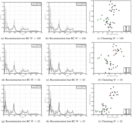
The selection of the window lengthW required more detailed analysis. To find the right parameter ofW the conclusions in§3.3 were followed. LargeW does not give a good reconstruction of the signal. An example of the different cases is given in Figure 5.

(8)

0 100 200 300 400 500 600 700 0 0.05 0.1 0.15 0.2 0.25 0.3 0.35 | Y | ( m / s 2) ω(Hz) Original

RC1−2

0 100 200 300 400 500 600 700

0 0.05 0.1 0.15 0.2 0.25 0.3 0.35 | Y | ( m / s 2) ω(Hz) Original

RC1−4

0.5 0.6 0.7 0.8 0.9 1 1.1 1.2 1.3

0 0.02 0.04 0.06 0.08 0.1 0.12

RC1 -(6 0 %variation)

R C 2 -( 8 % v a r ia ti o n ) B1 B2 B3 B4 B5

(c) ClusteringW = 100

0 100 200 300 400 500 600 700

0 0.05 0.1 0.15 0.2 0.25 0.3 0.35 | Y | ( m / s 2) ω(Hz) Original

RC1−2

(d) Reconstruction two RCW = 50

0 100 200 300 400 500 600 700

0 0.05 0.1 0.15 0.2 0.25 0.3 0.35 | Y | ( m / s 2) ω(Hz) Original

RC1−4

(e) Reconstrcution four RCW = 50

0.8 0.9 1 1.1 1.2 1.3 1.4 1.5

0 0.02 0.04 0.06 0.08 0.1 0.12

(f) ClusteringW = 50

0 100 200 300 400 500 600 700

0 0.05 0.1 0.15 0.2 0.25 0.3 0.35 | Y | ( m / s 2) ω(Hz) Original

RC1−2

(g) Reconstruction two RCW = 25

0 100 200 300 400 500 600 700

0 0.05 0.1 0.15 0.2 0.25 0.3 0.35 | Y | ( m / s 2) ω(Hz) Original

RC1−4

(h) Reconstrcution four RCW = 25

1 1.1 1.2 1.3 1.4 1.5 1.6 1.7 1.8

0.02 0.04 0.06 0.08 0.1 0.12 0.14 0.16

[image:8.595.74.526.203.624.2]

(i) ClusteringW = 25

(9)

0 100 200 300 400 500 600 700 0

0.05 0.1 0.15 0.2 0.25 0.3 0.35

|

Y

|

(

m

/

s

2)

ω(Hz)

Original RC1₋2

0 100 200 300 400 500 600 700

0 0.05 0.1 0.15 0.2 0.25 0.3 0.35

|

Y

|

(

m

/

s

2)

ω(Hz)

Original RC1₋4

1.1 1.2 1.3 1.4 1.5 1.6 1.7 1.8 1.9 −0.03

−0.02 −0.01 0 0.01 0.02 0.03 0.04 0.05 0.06 0.07

R

C

2

-(

5

%

v

a

r

ia

ti

o

n

)

B1

B2

B3

B4

B5

[image:9.595.80.516.88.489.2]

(c) ClusteringW = 7

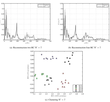
Figure 6: Damage assesstment with window lengthW = 7. The resolution of the signal was fixed at1.6s

long and sampled at640Hz

5 Conclusions

(10)

References

[1] Hoon Sohn, Charles R Farrar, Francois M Hemez, Devin D Shunk, Daniel W Stinemates, Brett R Nadler, and Jerry J Czarnecki. A review of structural health monitoring literature: 1996-2001. Los Alamos National Laboratory, NM,(2004).

[2] Nina Golyandina, Vladimir Nekrutkin, and Anatoly A Zhigljavsky.Analysis of time series structure: SSA and related techniques. CRC Press, 2010.

[3] A-M Yan, Gaetan Kerschen, Pascal De Boe, and J-C Golinval. Structural damage diagnosis under varying environmental conditions part I: a linear analysis.Mechanical Systems and Signal Processing, 19(4):847864, 2005

[4] A-M Yan, Gaetan Kerschen, Pascal De Boe, and J-C Golinval. Structural damage diagnosis under varying environmental conditions part II: local pca for non-linear cases. Mechanical Systems and Signal Processing, 19(4):847864, 2005

[5] Ian T Jolliffe.Principal component analysis.Volume 487. Springer-Verlag New York, 1986.

[6] DS Broomhead and Gregory P King.Extracting qualitative dynamics from experimental data.Physica D: Nonlinear Phenomena, 20(2):217-236, 1986.

[7] Robert Vautard and Michael Ghil.Singular spectrum analysis in nonlinear dynamics, with applications to paleoclimatic time series.Physica D: Nonlinear Phenomena, 35(3):395424, 1989.

[8] Hossein Hassani and Anatoly Zhigljavsky.Singular spectrum analysis: methodology and application to economics data.Journal of Systems Science and Complexity, 22(3):372394, 2009.

[9] Alexander Basilevsky and Derek PJ Hum. Karhunen-loeve. Analysis of historical time series with an application to the plantation births in Jamaica. Journal of the American Statistical Association, 74(366a):284290, 1979.

[10] David Garcia and Irina Trendalova.A multivariate data analysis approach towards vibration analysis and vibration-based damage assessment. Application for delamination detection in a composite beam.

Journal of Sound and Vibration, 2014.In press.

[11] V Moskvina and A Zhigljavsky.Application of the singular spectrum analysis for change-point detec-tion in time series.Journal of Time Series Analysis, submitted, 2001.

[12] Hossein Hassani.Singular spectrum analysis: methodology and comparisonJournal of Data Science 5(2007), 239-257.

[13] FJ Alonso, JM Del Castillo, and P Pintado.Application of singular spectrum analysis to the smoothing of raw kinematic signals.Journal of biomechanics, 38(5):1085-1092, 2005.