Bayesian Inference in a Cointegrating Panel Data Model
∗Gary Koop
Department of Economics University of Strathclyde
Roberto Leon-Gonzalez Department of Economics
University of Leicester [email protected]
and
Rodney Strachan Department of Economics
University of Leicester [email protected]
January 2006
Abstract:
This paper develops methods of Bayesian inference in a cointegrating panel data model. This model involves each cross-sectional unit having a vector error correction representation. It isßexible in the sense that different cross-sectional units can have different cointegration ranks and cointegration spaces. Furthermore, the parameters which characterize short-run dynamics and deter-ministic components are allowed to vary over cross-sectional units. In addition to a noninformative prior, we introduce an informative prior which allows for information about the likely location of the cointegration space and about the degree of similarity in coefficients in different cross-sectional units. A collapsed Gibbs sampling algorithm is developed which allows for efficient posterior inference. Our methods are illustrated using real and artiÞcial data.Keywords:
Bayesian, panel data cointegration, error correction model, reduced rank regression, Markov Chain Monte Carlo.JEL Classi
Þ
cation
: C11, C32, C33∗Address for correspondence: Rodney Strachan, Department of Economics, University of Leicester, LE1 7RH Leicester,
1
Introduction
The growing availability of panel data with largeT dimension (i.e. where the number of time series ob-servations is large) has stimulated a growth in research, both empirical and theoretical, which discusses time series issues in panel data models. Of particular interest are issues relating to nonstationarity and cointegration. In this paper, we develop a Bayesian approach to the analysis of cointegration in panels. We use a modelling framework which allows for great ßexibility in the way heterogeneity across cross-sectional units is incorporated. In particular, we allow for both cointegrating vectors and ranks to vary overN. Our use of Bayesian methods allows for the cointegrating ranks to be treated as random variables. Thus, our methods can either be used to select a particular model with speciÞed cointegrating ranks or to average across different cointegrating ranks. We also consider restricted models of interest (e.g. where all cross-sectional units have the same cointegrating rank). The use of Bayesian methods requires elicitation of a prior. We develop two priors, a noninformative and an informative one. The latter allows for the incorporation of prior beliefs that the same cointegrating relationship exists for all cross-sectional units. Furthermore, it allows for what we call "soft homo-geneity" restrictions (i.e. that comparable parameters in different cross-sectional units are likely to be similar to one another). We derive efficient methods of posterior analysis in our class of models and illustrate our methods using artiÞcial data and an application involving a monetary exchange rate model (see Groen, 2000 and Groen and Kleibergen, 2003).
The importance of this area of research is evidenced by the increasing tendency for researchers to employ panels of nonstationary processes in empirical studies in macroeconomics and international economics. For instance, the survey paper by Baltagi and Kai (2000) identiÞes many areas of applica-tion, including purchasing power parity (PPP), growth convergence and international R&D spillovers. To give one example which illustrates the issues which can be addressed through the use of panel data consider Jacobson, Lyhagen, Larsson and Nessén (2002). These authors use a multivariate panel cointegration model and demonstrate that, although strong purchasing power parity restrictions are rejected, the location of the cointegrating space is similar for all countries considered. This provides some evidence in support of PPP.
In terms of the frequentist econometric literature, there have been a range of methods proposed to obtain inference relating to cointegration in panel data models. Among many others, we note that residual-based, LM and likelihood based tests have been proposed by Kao (1999), McCoskey and Kao (1998), Pedroni (2004), Larsson, Lyhagen and Löthgren (2001) and Groen and Kleibergen (2003). The estimation methods used in these papers vary from OLS through maximum likelihood and generalized method of moments. The extent of this literature prevents us giving even a reasonable coverage here and so we refer the reader to the surveys by Phillips and Moon (2000) and Baltagi and Kao (2000).
reasonably well in Þnite samples, and is even preferable to some consistent estimators when Þnite sampling performance is considered. Although they impose a stability condition, thus precluding discussion of issues relating to unit roots and cointegration, this assumption could be relaxed (see also Hsiao and Pesaran, 2004). Li (1999) investigates PPP by considering support for symmetry and proportionality restrictions in the PPP relationship. She allows for stationary AR(1) errors in the relationship between log exchange rates and prices. Interestingly, while this paper does not explicitly consider cointegration, with one small change the model of Li could - using a triangular setup as proposed by Phillips (1991) - be easily extended to allow investigation of whether or not cointegration between log exchange rates and prices occurs.
We are aware of only one paper explicitly proposing a Bayesian approach to estimation of a cointegrating system in panel data models. Carmeci (2005) presents a state space model which implies cointegration by directly modeling the common stochastic trends. Under the assumption that the cointegrating rank is known and assumed equal in every cross-sectional unit, the author develops Bayesian methods for estimation. We are not aware of any paper that presents a fully Bayesian method of inference on cointegration in panels, when the cointegrating rank is unknown and may differ across cross-sectional units. The present paper attempts to address this gap in the literature.
The remainder of the paper is organized as follows. Section 2 introduces the model and describes the elements of Bayesian analysis: likelihood, priors and methods of posterior simulation. Section 3 illustrates our methods using artiÞcial data and Section 4 demonstrates the ßexibility of inference in the application used in Groen and Kleibergen (2003), which involves an interesting set of restrictions implied by economic theory. Section 5 concludes.
2
The Models
In a standard time series framework, cointegration is typically investigated using a vector error cor-rection model (VECM). To establish notation, to investigate cointegrating relationships involving an n-vector,yt,we write the VECM for t= 1, .., T as:
∆yt=Πyt−1+
l
X
h=1
Γh∆yt−h+Φdt+εt (1)
where then×nmatrixΠ=αβ0, whereαandβaren×rfull rank matrices andd
tdenotes deterministic
terms.1 The value of r determines the number of cointegrating relationships. εt is a Normal mean
zero error with positive deÞnite covariance matrix.
Before extending (1) to the panel data case, it is important to digress brießy to motivate an important issue in Bayesian analysis of cointegrated models. The VECM suffers from both local and global identiÞcation problems. The local identiÞcation problem occurs since, if α = 0, β does not appear in the likelihood function. The global identiÞcation problem can be seen by noting that
1The exact form of the deterministic terms is not crucial to our derivations so we leave these unspeci
Π = αβ0 and Π = αGG−1β0 are identical for any nonsingular G. This indeterminacy is commonly surmounted by imposing the so-called linear normalization where β = [Ir B0]0. However, there are
some serious drawbacks to this linear normalization (see Strachan and Inder, 2004 and Strachan and van Dijk, 2004b). Researchers in thisÞeld (see Strachan and Inder, 2004, Strachan and van Dijk, 2004b and Villani, 2005a,b) point out that it is only the cointegration space that is identiÞed (not particular cointegrating vectors) and that, for most purposes (including prior elicitation), it is preferable to think in terms of the cointegration space. Accordingly, we introduce notation for the space spanned by β, p=sp(β).
We can generalize (1) to the panel data case by includingisubscripts to denote the cross-sectional unit which we refer to as the ”individual” hereafter (wherei= 1, .., N). That is,yi,tis annvector of
observations on the dependent variables for individualiat timet2 and the panel VECM is written as:
∆yi,t=Πiyi,t−1+
li
X
h=1
Γi,h∆yi,t−h+Φidi,t+εi,t (2)
where nowΠi =αiβ0i whereαi and βi aren×ri full rank matrices. Our model allows for the number
of cointegrating relationships to vary across individuals and thus, we extend our previous notation such that the cointegration spaces are now pi =sp(βi). The covariance matrices for vectors εi,t are
assumed to be
E¡εi,tε0j,s
¢
=
½ Σij
0
fort=s
fort6=s . (3)
In other words, we are assuming the errors to be uncorrelated over time, but correlated across equa-tions for a given individual and correlated across individuals. Note that the last assumption differs from much of the previous literature. For instance, Larsson, Lyhagen and Löthgren (2001) use a more restrictive model assuming E³εi,tε0j,s
´
= 0ifi6=j for all tands. Although allowing for a correlation between errors for different individuals is not usually done with microeconomic survey data, with macroeconomic panels where the ”individuals” are countries such a correlation is potentially impor-tant.We are therefore following the more general model of Groen and Kleibergen (2003) which does allow for such a correlation. Note also that our model is more ßexible than the one of Groen and Kleibergen (2003) in that we relax the assumption of a common cointegrating rank.
There are many features of (2) that the researcher might be interested in. For each individual, we would naturally be interested in the dimension of the cointegrating space,ri, and whetherri =r for
alli.Other questions of interest relate to the cointegrating spaces,pi=sp(βi). A restricted version of
(2) would have the same cointegrating relationships (i.e. the sameri andβi) for every individual and,
thus, pi = p. Alternatively, if different individuals have different numbers of cointegrating vectors,
then we might be interested in whether all of the cointegrating spaces lie within some more general one. That is, ifri ≤r fori= 1, .., N and p is a cointegration space with dimensionr, then we might
be interested in investigating whetherpi ⊆p fori= 1, .., N.
2It is not complicated to allow fory
i,tto be of dimensionni, but we will assumeni=n,for simplicity. Similarly it is
As a simple illustration of how these questions might arise, consider the balanced growth hypothesis in the real business cycle model presented by King, Plosser, Stock and Watson (1991). Assume yi,t = (ci,t, ai,t, gi,t)0 whereci,t is log consumption for countryi, ai,t is log investment for that country
and gi,t is log income. If the elements of the vectoryi,t areI(1)and are cointegrated then 0< ri <3.
If there are two cointegrating relationships (ri = 2) and the logs of the great ratios of consumption
to income and investment to income are stable such that ci,t−gi,t and ai,t−gi,t are I(0) in every
country, then the cointegrating space, pi, is
pi =p=sp
⎛
⎝ 10 01 −1 −1
⎞ ⎠.
In an empirical analysis using panel data, it would be of interest to investigate this restriction (i.e. whether two cointegrating vectors exist for each country and whether their values are consistent with the great ratios). However, it is possible that some countries might only have one cointegrating relationship, so that ri = 2 for some countries and ri = 1 for others. In this case, investigating
whether pi = p for all i = 1, .., N is not reasonable. Instead, the researcher may be interested in
investigating whether the cointegrating relationships either involve the great ratios individually (for ri = 2) or involve a linear combination of the (logs of) the great ratios. In terms of our notation, this
involves investigating whetherpi ⊆p fori= 1, .., N.
In most empirical applications, the cointegrating spaces will be of most interest and, hence, the researcher will be most interested in a set of models deÞned by restrictions on these. However, it is also common for the set of models to be broadened by considering different forms of the deterministic processes, di,t, and the number of lags li and it might be desirable to allow these to vary across
individuals. Thus, in empirical work, the researcher might want to consider a very wide range of models indeed. However, in order to focus on the central issues relating to cointegration, we will assume a common lag length for all individuals (i.e. li=lfor alli) and common deterministic process
(i.e. di,t=dtfor all i) and develop methods of inference forri and p.
2.1
The Likelihood Function
In this section we show two representations of the likelihood, involving different parameterizations, which we draw on in our discussion of posterior simulation. Note that the matrix of long run multipliers can be written as:
βiα0
i = [βiκi]£αiκ−i1
¤0
≡β∗iA0
i (4)
whereβiis restricted to be semi-orthogonal (for reasons described in the next section) andκiis positive
deÞnite and deÞned so thatAiis semi-orthogonal. Here we have usedβ∗i =βiκi andαi =Aiκ0i. There
are many choices forκi which satisfy these properties, but a convenient one we will use here is:
κi =¡α0iαi¢ 1
2 =¡β∗0 i β∗i
¢1
For reasons explained below, our posterior simulator will involve switching between the parameteriza-tions in (4).
To establish notation, we collect the n×n blocks Σij into the N n×N n matrix Σ = {Σij}.
Collecting the (n×1) vectors εi,t into (T ×n) matrices εi = (εi,1, . . . , εi,T)0, then collecting these
matrices into the(T ×Nn) matrixε= (ε1, . . . , εN),we obtaine=vec(ε) being the vector of errors.
This vector has covariance matrix
E¡ee0¢=V
e= (Σ⊗IT). (6)
The density of the errors, a key building block in forming the likelihood for this model, is then
|Σ|−T /2exp
½
−12e0¡Σ−1⊗I
T¢e
¾
=|Σ|−T /2exp
½
−12trΣ−1ε0ε
¾
.
We next give two representations fore that will prove useful in developing a sampling scheme for the parameters.
We rewrite (2) by deÞningzi,t=β0iyi,t−1, the1×(k+ri)vectorXi,t=
³
z0
i,t,∆yi,t0 −1, . . . ,∆y0i,t−l, d0t
´
, where k is the number of deterministic terms plus n times the number of lags (assumed to be com-mon to all individuals and, hence, we have not included an isubscript), and the (k+ri)×n matrix
Bi = (αi,Γi,1, . . . ,Γi,l,Φi)0 and, thus,
∆y0
i,t =Xi,tBi+ε0i,t. (7)
If we stack the vectors in (7) overtas∆yi = (∆yi,1, ...,∆yi,T)0 andXi=
³
Xi.01, ..., Xi.T0 ´0 then, we can write ∆yi=XiBi+εi. Vectorizing this equation gives us the form
vec(∆yi) = (In⊗Xi)vec(Bi) +ei
oryi = xibi+ei
where yi =vec(∆yi), xi = (In⊗Xi), bi =vec(Bi) and ei =vec(εi) such that E
³
eie0j
´
=Σij⊗IT.
We collect the vectors yi and bi into the vectors y = (y10, . . . , y0N)0, and b = (b01, . . . , b0N)0, and deÞne
the matrixxas the T N n×N n(k+r)(where r=
rN i=1ri
N ) block diagonal matrix with diagonal equal
to(x1, ..., xN). Using these deÞnitions, we can express the full system of equations asy−xb=e. The
likelihood can now be expressed as
L(b,Σ, β) = |Σ|−T /2exp
½
−1
2(y−xb) 0V−1
e (y−xb)
¾
(8)
= |Σ|−T /2exp
½
−1 2
∙
s2+³b−bb´0V−1³b−bb´¸¾
where s2 =y0M
Vy, MV =Ve−1−Ve−1xV x0Ve−1,bb=V x0Ve−1y, Ve = (Σ⊗IT) and V =¡x0Ve−1x
Our next representation of the likelihood demonstrates that we can obtain a Normal form for the cointegrating vectors (conditional on the other parameters of the model). That is, the conditional pos-terior density of the vectorbβ∗=
³
b0
β∗,1, . . . , b0β∗,N
´0
, wherebβ∗,i=vec(β∗i), can be shown to be Normal.
To do this let us again rewrite (2) but this time deÞne the1×kvectorwi,t=
³ ∆y0
i,t−1, . . . ,∆yi,t0 −l, d0t
´
, and thek×nmatrixCi = (Γi,1, . . . ,Γi,l,Φi)0 and, thus,
∆y0
i,t=y0i,t−1β∗iAi0+wi,tCi+ε0i,t. (9)
If we stack the vectors overtas∆yi= (∆yi,1, ...,∆yi.T)0,yi,−1 = (yi,0, ..., yi,T−1)0andwi =
³
w0i,1, ..., w0i,T´0, then we can write∆yi=yi,−1β∗iA0i+wiCi+εi. Vectorizing this equation we obtain
vec(∆yi−wiCi) = (Ai⊗yi,−1)vec(β∗i) +vec(εi)
orybi = bxibβ∗,i+ei
where ybi =vec(∆yi−wiCi),and bxi = (Ai⊗yi,−1). Now stack the vectors byi into by = (yb10, . . . ,ybN0 )0
and deÞne bx as the T Nn×N nr block diagonal matrix with diagonal equal to (xb1, ...,bxN) so we can
express the system of equations asyb−xbb β∗ =e. The likelihood can now be expressed as
L(b,Σ, β) = |Σ|−T /2exp
½
−12¡by−xbb β∗¢0Ve−1¡yb−xbb β∗¢
¾
(10)
= |Σ|−T /2exp
½
−1 2
∙
s2β∗+
³
bβ∗−bbβ∗
´0 Vβ−∗1
³
bβ∗−bbβ∗
´¸¾
wheres2β∗ =yb0MVβ∗y, Mb Vβ∗ =V− 1
e −Ve−1bxVβ∗xb0Ve−1,bbβ∗ =Vβ∗xb0Ve−1by,and Vβ∗ =
¡ b
x0V−1
e xb
¢−1
. This representation of the likelihood shows that the form of the posterior for bβ∗ (conditional upon the Ci
and Σ) is Normal if the (conditional) prior forbβ∗ is Normal.
2.2
Priors
In this section, we describe two classes of priors which may be useful for empirical research. TheÞrst of these is a noninformative prior, suitable for reference or benchmark purposes. The second is an informative prior which contains what we call "soft homogeneity" restrictions. That is, in many cases economic theory suggests that the cointegration space should be the same for different individuals and of a particular form. In an empirical analysis, the researcher might not want to impose this sort of homogeneity in a strong sense, but, through the use of priors, we can do so in a soft sense. That is, rather than setting parameters to have the same values for all individuals, we specify common informative priors that favour parameter values which are similar for different individuals. This is likely to be of particular beneÞt since our model contains many parameters and, thus, issues relating to possible over-parameterization and efficiency of estimation are likely to be important.
which attempt to surmount the problems this causes (see the survey paper by Koop, Strachan, van Dijk and Villani, 2005). We will not recreate the arguments of this literature in detail here. Suffice it to note that it is unsatisfactory to use some apparently sensible approaches. For instance, atÞrst sight it seems sensible just to use a standard prior (e.g. aßat prior or a Normal one) onBafter imposing the linear normalizationβ = [IrB0]0. As discussed in Kleibergen and van Dijk (1994), the local non-identiÞcation
of the model causes problems for this sort of Bayesian approach. The issue here is that when α has reduced rank (e.g.,α= 0) the conditional posterior distribution forB|αis equal to its prior (i.e. since B does not enter the likelihood function at the point α= 0 there is no data-based learning aboutB and, thus, its posterior equals its prior at this point). If the prior forB|α= 0is improper (as it is in the common “noninformative” case), then the posterior will also be improper. Formally, Kleibergen and van Dijk (1994) associate the local non-identiÞcation problem with nonexistence of posterior moments and non-integrability of the posterior (under a common noninformative prior). Kleibergen and van Dijk (1998) additionally point out that local non-identiÞcation implies an absorbing state in a Gibbs sampler, thereby violating the convergence conditions for the sampler.
With regards to global identiÞcation, Strachan and Inder (2004) show how the use of linear iden-tifying restrictions places a restriction on the estimable region of the cointegrating space. This paper also provides an extensive discussion of further problems associated with the use of linear identifying restrictions. Strachan and van Dijk (2004b) show that a ßat and apparently “noninformative” prior on B in the linear normalization favors regions of the cointegration space near where the linear nor-malization is invalid. Hence, the linear nornor-malization is used under the assumption that it is valid while at the same time the prior says that the normalization is likely to be invalid.
Coming out of this literature is the strong message that prior elicitation should be made directly off the cointegration space itself (which is all that is identiÞed). Several papers, including Strachan (2003), Strachan and Inder (2004) and Villani (2005a,b) propose various approaches which involve such a focus. In this paper, we extend the general framework outlined in Strachan (2003) and Strachan and Inder (2004) to our panel cointegration model. The advantages of this approach are that they allow us to avoid identiÞcation restrictions that may restrict the estimable cointegration space, allow for priors which are, in a sense, noninformative (but are proper and, hence, allow for calculation of posterior odds ratios) and offer a convenient framework for incorporating prior information (if the researcher wishes to incorporate it).
governing the direction ofβ and thereforep.
To extend these intuitive concepts to general n and r, some additional deÞnitions are required. Our aim is to provide a rigorous deÞnition of the intuitive idea of assigning equal prior probability to every possible cointegration space of dimension r. As described in Strachan and Inder (2004), having β being semi-orthogonal such that β0β =I
r identiÞes the cointegrating vectors without placing any
restrictions on the cointegrating space. The set of all n×r semi-orthogonal matrices is called the Stiefel manifold Vn,r. The Stiefel manifold is a compact space and admits a Uniform distribution.
In the case where r = 1, one might conceptualize the collection of directions of all n-dimensional unit vectors, β ∈ Vn,1, as describing ann-dimensional unit sphere centered at the origin. Thus, we
may visualize a Uniform distribution on the n-dimensional unit sphere as characterizing a Uniform distribution onVn,1. Forr >1,we can think of each vector in β as describing a unit sphere with the
additional restriction that the vectors are all orthogonal to each other.
The Grassman manifold Gn,r is the abstract space of all possible r-dimensional planes of Rn.
The cointegration space is an element of the Grassman manifold, that is p ∈ Gn,r. In the VECM
only the space spanned by the columns of β is identiÞed, such that we only have information on p = sp(β) ∈ Gn,r. A Uniform prior for the cointegration space is therefore given by the Uniform
distribution onGn,r.
For calculating posterior odds ratios, proper priors are required to avoid Bartlett’s paradox (see Bartlett, 1957). But, since β now has a compact support, the prior over the cointegration space is proper. Formally, this approach uses the natural relationship between the Grassman manifold and the Stiefel manifold and the development of measures on these spaces presented in James (1954). In particular, a key result is that the Uniform distribution onVn,r induces a Uniform distribution onGn,r
(see James, 1954, and Strachan and Inder, 2004). Thus, it is possible to work with the semi-orthogonal matrices, i.e. β ∈Vn,r, and adjust all integrals to account for the fact that Vn,r is a larger space than Gn,r.
In this paper, we have only sketched out the basic ideas relating to prior elicitation in the cointe-gration models, and refer the reader to the literature we cite above for further details. Suffice it to note here that, in this paper, we extend these ideas to work with the panel cointegration model.
2.2.1 A Noninformative Prior
Let bβ =
³
b0
β,1, . . . , b0β,N
´0
, where bβ,i = vec(βi), contain all the parameters which determine the
cointegration spaces. The remaining parameters of the model areΣandb, wherebis deÞned between (7) and (8). Noting that, conditional upon bβ, the model reduces to a linear one (see equation 7), a
plausible candidate is the standard noninformative prior for multivariate linear models:
p(b,Σ, bβ)∝|Σ|−(Nn+1)/2, (11)
where we add the additional restriction, arising from our wish to be noninformative about the coin-tegrating space and have an identifying restriction which does not limit that space, that βi is semi-orthogonal such thatβ0
Note, however, that although the marginal prior for bβ is proper, the joint prior for all the
para-meters is improper. The impropriety relating to the prior for Σis not a problem, since it is common to all models.3 However, a proper prior would be required for the remaining parameters should we wish to calculate posterior odds ratios comparing different cointegrating ranks. That is, if we wish to estimate a single model for speciÞed values for ri (and speciÞed values for l and dt) the prior given
in (11) will be appropriate. However, if we are wishing to compare this single model to another with different values for ri (and/or different values forl and dt), then an informative prior for b would be
required. It is to such an informative prior to which we turn. However, it is worth noting in passing that a researcher who is interested in model comparison, but would prefer to avoid informative priors, could use information criteria to approximate marginal likelihoods or could adopt a training sample approach. That is, (11) could be used as a noninformative prior which is then combined with a training sample (e.g. the initial 10% of the data) to yield a "posterior". This "posterior" can then be used as an informative prior in a posterior analysis involving the rest of the data. See O’Hagan (1995) for a discussion of such an approach.
2.2.2 An Informative Prior (including soft homogeneity restrictions)
In many cases the researcher may wish to specify an informative prior on the cointegrating space. For instance, in our previous example arising from King, Plosser, Stock and Watson (1991), the researcher may wish to elicit a prior which implies that the cointegrating space lies in the region implied by the great ratios. Alternatively, the researcher may wish to elicit a prior which implies that the cointegration spaces (or other parameters) for different individuals are similar. We refer to the latter as soft homogeneity restrictions. In addition, in order to avoid the issues relating to Bartlett’s paradox discussed in the previous section, the researcher may wish to elicit an informative prior forb. Here we describe an approach to prior elicitation which incorporates these aspects.
Some aspects of our prior are best motivated in the context of our posterior simulation algorithm. Hence, we digress brießy to informally discuss computation. Posterior computation is greatly compli-cated by the fact thatβi is semi-orthogonal which precludes use of the simple Gibbs sampling methods described, e.g., in Geweke (1996). For the non-panel cointegration model, Koop, Leon-Gonzalez and Strachan (2005) develop an efficient method of posterior simulation based on the idea of a collapsed Gibbs sampler developed in Liu (1994) and Liu, Wong and Kong (1994). To give some preliminary intuition for this, consider the relationships deÞned in (4). For prior elicitation or posterior computa-tion, we may consider either(βi, αi) or(βi∗, Ai).Crucially, in theÞrst of these parameterizations,βi is
semi-orthogonal whileαi is unrestricted, whereas in the second it isβ∗i which is unrestricted whereas
Ai is semi-orthogonal. In the next section we develop a collapsed Gibbs sampler which alternates
between these two parameterizations. Arguments made in Liu (1994) and Liu, Wong and Kong (1994)
3When calculating posterior odds ratios, it is common to make use of improper, noninformative priors over parameters
prove that this will be more efficient than a Gibbs sampler which works only with(βi, αi)or(β∗i, Ai).
Even more crucially, with the priors developed in this section, the collapsed Gibbs sampler will only involve draws from the Normal distribution (and inverted Wishart4forΣ), enormously simplifying the computational burden.
We now turn to our informative prior and begin by discussingbandΣ. Typically, these parameters will be of less importance in an empirical exercise than the prior on the cointegrating space. ForΣwe maintain the noninformative prior given in (11), although an inverted-Wishart form could also easily be handled. For bwe assume:5
b∼N
µ
0, V1 ν
(12)
where ν is a scalar which controls the degrees of informativeness or precision of the prior. Note that ν can be interpreted as a shrinkage parameter and, thus, (12) shares some similarities with shrinkage priors commonly used in the VAR literature (see, e.g., Litterman, 1986). Note, however, that we treat ν as a parameter (rather than a hyperparameter selected subjectively by the researcher).
Now consider the prior covariance matrix (up to the scalar shrinkage parameter) V in (12). Of course, any choice forV can be made. Here we motivate a particular form for the elements ofV which relate to αi or, equivalently, Ai. Considering the relationships in (4) and surrounding discussion, it
makes sense, analogous to our noninformative prior for the semi-orthogonal βi, to assume that the n×ri semi-orthogonal matrices(Ai, ..., AN) are a priori independent and that:
p¡Ai, ..., AN|τ , v, bβ∗
¢
∝1 (13)
as this implies a Uniform but proper density for each of subspaces deÞned by the Ai fori= 1, .., N.
Given the relationships in (4) we can derive a prior for (β∗i, Ai)from a prior for(βi, αi) or vice versa.
The prior (13), along with the prior forβi (to be deÞned shortly), implies that
vec(αi)|τ , βi, ν ∼N
µ
0,1 ν
¡
β0
iPτ−1βi
¢−1 ⊗In
, (14)
and, thus, that the diagonal blocks ofV that correspond toαi are equal to¡β0iPτ−1βi
¢−1
⊗In(wherePτ
will be deÞned shortly). The remaining elements ofV, corresponding to the parameters (C1, ..., CN),
can be speciÞed using either informative or noninformative choices and will be further discussed below. For the cointegration spaces, pi (and therefore for βi) it is often desirable to have a prior which
allows for a common location across individuals. If an economist believes a parameter is likely to have a particular value, she will often place more prior mass around this likely point. To extend this idea from parameters to spaces, some new ideas are required. To provide some intuition, consider the case where we have a prior belief that the space of βi should be approximately the space of H where H is semi-orthogonal and is of the same dimension as βi (we will extend this to allow H to have a different number of columns from βi below). To obtain the semi-orthogonal matrix H the researcher
4See, e.g., Bauwens, Lubrano and Richard (1999), page 305 for a de
Þnition of the inverted Wishart distribution.
5
canÞrst specify the matrix Hg containing desired coefficient values and then use the transformation H=Hg(Hg0Hg)−1/2
.The matrixH constructed in this way will span the same space asHg but will be semi-orthogonal.
For instance, if, motivated by King, Plosser, Stock and Watson (1991), we wanted a prior reßecting the fact that the great ratios are probably cointegrating relationships, we would set:
Hg =
⎛ ⎝
1 0
0 1
−1 −1
⎞ ⎠.
Hg is not semi-orthogonal butH =Hg(Hg0Hg)−1/2 will be (and will span the same space).
A dogmatic prior would be obtained by setting βi =H which places all of the prior mass for pi
at pH = sp(H). Strachan and Inder (2004) develop an informative, but non-dogmatic prior, for the cointegration space and we adopt a similar approach here. Intuitively, we want a prior which says the cointegration spaces,pi, are likely to be close topH =sp(H) and, thus, farthest frompH⊥ =sp(H⊥)
where H⊥ is the orthogonal complement of H.The pis are weighted averages of pH and pH⊥ and we
can elicit a prior about these weights.
One way to motivate our informative prior is through its implications for β∗i. To this end, suppose we have an n×ri matrixZi with all elements being i.i.d. N¡0, ν−1¢. A standard result tells us that
the space of Zi will be Uniformly distributed over the Grassman manifold. If we simply set β∗i =Zi
and used this as a prior for β∗i then it would be noninformative over the cointegrating space. To get a dogmatic informative prior for β∗i (and, thus, the cointegrating space), we can project Zi into
pH. Another standard result in matrix algebra says this projection is given by β∗i =HH0Z
i. At the
opposite extreme, we could project Zi intopH⊥ as βi∗ =H⊥H⊥0 Zi if we wanted a cointegration space
as far away frompH as possible. A non-dogmatic informative prior can be introduced by introducing the random variableη (with distribution centered at 0) which centers the prior overpH, but attaches weight to other spaces as:
β∗i = HH0Z
i+ηH⊥H⊥0 Zi
= PηZi
wherePη =HH0+ηH⊥H⊥0 .
Using the properties of the Normal distribution, it follows that
vec(β∗i)|η, ν ∼N
µ
0, Iri⊗ 1 νPηP
0
η
.
But, given the structure ofPη, it follows thatPηPη0 =HH0+η2H⊥H⊥0 =Pη2. Thus,ηenters the prior
only through η2 and, accordingly, we introduce the notationτ =η2 and use the following conditional Normal prior for β∗i:
vec(β∗i)|τ , ν ∼N
µ
0, Iri⊗ 1 νPτ
or, equivalently,
bβ∗|τ , ν ∼N
µ
0,1 νVβ∗
(16)
whereVβ∗ =diag(Iri ⊗Pτ). 6
This prior will more strongly weight the cointegrating space towardsH the closer τ is to zero. At τ = 1, this prior is Uniform over the Grassman manifold (since Pτ=1 = In) and τ > 1 implies more
weight towards the space ofH⊥.Therefore, it is sensible to either truncate the distribution ofτ to the region(0,1]or to choose the hyperparameters in the prior for τ so thatτ >1is a very unlikely event. Note that our informal motivation implicitly assumedHto be of the same dimension asβ. However, if we deÞneH∈Vs,n to be a knownn×s(s≥ri)matrix andH⊥∈Vn−s,nits orthogonal complement,
then our prior expresses the belief that the cointegration spacepi is likely to be included in the higher
dimensional space pH.7
For any p(τ) and p(ν), we can write the joint prior for β∗i and (ν, τ) as
p(ν)p(τ)
µ
2π ν
¶−N nr/2
τ−N(nr−r2)/2expn−ν 2Σ
N
i=1trβ∗i0Pτ−1β∗i
o
= p(ν)p(τ)
µ
2π ν
¶−N nr/2
τ−N(nr−r2)/2expn−ν 2Σ
N
i=1trβ∗i0HH0β∗i
o
×expn− ν 2τΣ
N
i=1trβ∗i0H⊥H⊥0 β∗i
o
, (17)
wherer2 = rNi=1r2i
N . In our empirical work, we select for p(ν) the form:
ν∼G³µν, νν−nN r´ (18)
whereG³µ
ν, νν −nN r
´
denotes the Gamma distribution with meanµ
ν and degrees of freedomνν−
nN r. Note that the degrees of freedom depends onnN r. This arises out of our wish to have the prior p(ν|β∗i = 0)the same for every model we consider in our model comparison exercise. Such a condition is necessary for using the Savage-Dickey density ratio as we do below. For brevity, we will not provide details, but it turns out that ifp(ν) has the form given in (18) then the resulting prior forν satisÞes the (reasonable and commonly-used) conditions for the Savage-Dickey density ratio to be used.
Using the transformations β∗i = βiκi and κiκ0i = with change of measure (dβ∗i) = 2−ri | |(n−ri−1)/2(d ) (dβ
i),and using (18) to integrate outν, we can obtain
p(τ , bβ) =p(τ)τ−N(nr−r 2)/2
ΠNi ¯¯β0
iPτ−1βi¯¯−n/2cr. (19)
6Note thatband b
β∗ share elements in common (i.e. κi) and therefore, the prior speciÞcation onbhas implications
on the prior ofbβ∗. This is the reason why the shrinkage parameter,ν, appears in 16. Note thatνdoes not affect the
marginal prior for cointegrating spaces.
7
wherecr = 2−NrπN(r
2−r)/4−Nnr/2
ΠNi Πri
j Γ[(n+ 1−j)/2].Since the cointegrating space pi is
identi-Þed given a value for β∗i, the expression in (17) or (19) can be regarded as the joint prior for(pi, τ)
conditional upon ri.
From the form in (17), a convenient form of prior forτ−1 that suggests itself is Gamma
τ−1 ∼G³µτ, ντ´
possibly truncated to [1,∞) to ensure τ <1. Alternatively, we could choose values, as we do in our application, such as µτ = 5 and ντ = 15 which will ensureP(τ <1)≈ 1.In the truncated case the normalizing constantcr in (19) is adjusted by dividing byP¡τ−1 >1¢.
Note that, if we use appropriate common values for µτ andντ for every individual, we will ensure that eachpi has its prior mass near topH =sp(H). This is an example of what we refer to as a soft
homogeneity restriction. That is, we are not restricting, a priori, each individual to have the same cointegration space, but we are expressing the view that different individuals are likely to have similar cointegration spaces. In general, such soft homogeneity restrictions can be imposed in two ways with this prior. First, priors (such as the prior for τ) can be the same or can share common locations. Second, we can choose V deÞned in (12) to have a structure which implies correlation between the same parameters for different individuals. Here we brießy describe one strategy for specifyingV. The N n(k+r)×N n(k+r)matrixV can be partitioned inton(k+ri)×n(k+ri)blocks on the diagonal
Vii, which can be chosen to have various forms (see equation 14 for the form relating to theα0
is). On
the off-diagonals, it would often make sense for the n(k+ri)×n(k+rj) matrices Vij to have zeros
in the rows and columns relating to the α0
is. Thus, no a priori correlation8 is assumed between the
α0
is. However, it will usually be sensible to assume thatvec(Ci)and vec(Cj) are positively correlated
with one another, a priori. This can be done by specifying the nk×nk matrix of prior covariances between the elements of vec(Ci) and vec(Cj) to be equal toρbInk, where0< ρb <1.
This completes our speciÞcation of an informative prior which has three key properties: i) It allows for prior information about the likely location of the cointegration space to be incorporated; ii) It allows for prior information about the degree of similarity in coefficients across individuals (which we refer to as soft homogeneity restrictions); iii) It contains a parameter ν which allows for shrinkage of coefficients on short run dynamics and deterministic terms.
2.3
Posterior Computation
Using the priors speciÞed above and the likelihood in (8) and (10), we can derive various posterior con-ditional densities of use in our posterior simulation algorithm. Using standard results (e.g., Bauwens, Lubrano and Richard, 1999, Chapter 9), the conditional posterior ofΣcan be conÞrmed to be inverted Wishart with degrees of freedom parameter T and scale matrix ε0ε, where ε is deÞned just after 6.
8If the cointegrating relations are exactly identiÞed, all individuals share the same cointegrating rank and the same
cointegrating relationship holds for all equations, then it would make sense to assume the adjustment coefficients (αi)
are a priori correlated. However, without these restrictions, it does not make sense to assume the columns ofαiandαj
Similar standard results can be used to obtain the posterior distribution forbconditional upon(Σ, bβ)
which is Normal with mean bb =V V−1bb and covarianceVb=£V−1+νV−1¤−1.
TheÞnal block in a standard Gibbs sampler would involve the cointegrating vectors,bβ = (b0β,1, . . . , b0
β,N)0, where bβ,i = vec(βi). Because of the semi-orthogonality of βi, this posterior conditional is
difficult to draw from directly. However, the conditional posterior distribution of bβ∗ turns out to
be Normal (we remind the reader that bβ∗ =
³
b0
β∗,1, . . . , b0β∗,N
´0
, where bβ∗,i = vec(β∗i)). To be
precise, recalling the deÞnition of Ci before equation (9), and deÞning ci = ¡vec(Ai)0, vec(Ci)0¢0
and c = (c0
1, . . . , c0N)0, the posterior distribution for bβ∗ conditional upon (Σ, c) is Normal with mean
bβ∗ =Vβ∗Vβ−∗1bbβ∗ and covarianceVβ∗ =
h
Vβ−∗1+νV−β∗1
i−1 .
In the process of drawing the parameters ¡Σ, b, bβ∗¢, we need to drawν and τ−1.The conditional
posterior distribution forν is Gamma with mean
µν =νν
h
(νν−nN r)/µν +b0V−1bi−1
and degrees of freedomνν =N nk+νν. The conditional distribution forτ−1 is Gamma with degrees
of freedomντ =ντ+N
¡
nr−r2¢and mean µ
τ =ντ
h
ντ/µ
τ +νΣ N
i=1trβ∗i0H⊥H⊥0 β∗i
i−1
.
From these conditional distributions we summarize the following sampling scheme using a collapsed Gibbs sampling method:
1. Initialize (b,Σ, bβ, ν, τ) =
³
b(0),Σ(0), β(0), ν(0), τ(0)´.
2. Draw Σ|b, bβ, ν, τ from IW³PNi=1ε0iεi, T
´
3. Draw b|Σ, bβ, v, τ from N
¡
bb, Vb
¢
4. Calculate Ai = (α0iαi)− 1 2 α
i and createc.
5. Draw bβ∗|c,Σ, v, τ from N¡bβ∗, Vβ∗¢.
6. Decompose eachβ∗i asβ∗i =βiκi using κi=¡β∗i0β∗i
¢1 2 andβ
i=β∗iκ−1. Constructαi =Aiκi.
7. Draw ν|b, bβ,Σ, τ from G(µν, νν).
8. Draw τ−1|b, b
β,Σ, v from G(µτ, ντ).
9. Repeat steps 2 to 8 for a suitable number of replications.
Note that, in this sampler, the transformations involving the long run multipliers are based on (5). To see why these steps suffice to set up a posterior simulator, we Þrst show that, conditional on (v, τ ,Σ), steps 3 to 6 deÞne a collapsed Gibbs sampler (Liu, 1994). To show this, note from (4) thatαi
can be decomposed into(Ai, κi), and that therefore the draw ofbin step 3 is a draw of (c, κ1, ..., κN).
Therefore, dropping for simplicity the conditioning arguments(v, τ ,Σ), the value ofcobtained in step 3 is a draw fromc|bβ, that is obtained marginally on (κ1, ..., κN). Similarly, the value of bβ obtained
in step 5 is a draw from bβ|c, (i.e. obtained again marginally on (κ1, ..., κN)). Therefore, steps 3 to
6 deÞne the collapsed Gibbs sampler suggested by Liu (1994) and Liu, Wong and Kong (1994), who show that this algorithm is more efficient than a standard Gibbs sampling algorithm (i.e. one which simply draws from the conditional posteriors of band bβ).
Finally, we extend the collapsed Gibbs sampler with steps that generate (κ1, ..., κN), Σ, v, and
τ from their corresponding conditional posterior densities and it is trivial to show that the posterior density continues to be the invariant distribution of the sampler. For a more detailed explanation of this algorithm in the context of a standard (non-panel) cointegration model see Koop, Leon-Gonzalez and Strachan (2005).
We will usually be interested in comparing different models nested within the general model deÞned above. For instance, we might wish to compare the unrestricted model with one where the same cointegrating rank holds for all individuals. We also might wish to calculate the posterior for ri for
i= 1, ..N. The Savage-Dickey density ratio (see, e.g., Verdinelli and Wasserman, 1995) proves to be a simple and efficient way of doing so. That is, it allows us to compute the Bayes factor comparing every model to a base model (e.g. the model where cointegration does not occur for any individual). This information can then be used to compare any two models, build up the posterior forri fori= 1, ..N,
do Bayesian model averaging or select a single model. To compute the Bayes factor for the modelMr
with a particular set of cointegrating ranks: r= (r1, r2, . . . , rN)against modelM0 withr = (0, . . . ,0), we note that the restricted case occurs when αi = 0. As αi and Πi have the same singular values
(which determine the rank of a matrix, e.g. Golub and van Loan, 1996), Πi = 0 occurs if and only
ifαi = 0. If we deÞne α= (vec(α1)0, ..., vec(αN)0)0, we can use the conditional posterior distribution
and (marginal) prior for αto compute the Savage-Dickey density ratio (SDDR):
B0,r =
p(α|Mr, y)|α=0 p(α|Mr)|α=0
(20)
Thus we can use output from our Gibbs sampler and the prior to estimate the required ratio:
b
B0,r =
1
MΣMm=1 p
³
α|Mr,Σ(m), C1(m), ..., C (m)
N , τ(m), ν(m), bβ, y´¯¯¯ α=0 p(α|Mr)|α=0
, (21)
wherem= 1, .., M denote the (post burn-in) Gibbs sampler replications and (m) superscripts denote the replications themselves (or, as below, functions of these replications).
We begin by deriving the analytical expression for p(α|Mr)|α=0. Using the properties of the
Gamma distribution and the MACG distribution (Chikuse, 1990), it can be shown that the marginal prior forαevaluated atα= 0is
p(α|Mr)|α=0=
Ã
2ντ µτ
!N(nr−r2)/2Γ
µ
N(nr−r2)+ν
τ 2
Γ(ντ/2)
Γ(νν/2)
Γ((νν −N nr)/2)
Ã
νν−N nr µνπ
This expression gives us the denominator of the SDDR. The numerator of the SDDR is the marginal posterior for α evaluated at zero. Using the fact that the posterior for b conditional upon (Σ, bβ) is
N(bb, Vb), it follows thatαisN(bα, Vα), wherebα andVα are given by the elements ofbband Vb that
correspond to α. Therefore, the Gibbs sampler can be used to estimate the numerator of the SDDR as:
(2π)−Nnr/2 M
M
X
m=1
¯ ¯
¯V(αm)¯¯¯−1/2exp
½
−21b(αm)0Vα(m)−1b(αm)
¾
.
There are other restricted versions of our general model in which the researcher may be interested. The Appendix describes how variants on the methods described above can be used to calculate Bayes factors relating to these models. Here we just list the restrictions of interest. Firstly, in practice it is often the case that there is interest in testing overidentifying restrictions of the form pi ⊆pH for
a subset of the countries i = 1, ..., N. This restriction can be imposed by writing βi = Hϕi, where ϕi∈Vri,s is an unknowns×ri full rank matrix. Our empirical example in the next section shows how such a restriction can arise. Secondly, we would also like to obtain the probability that all countries have the same unknown cointegrating space p = sp(β). Finally, the Appendix also describes how to calculate the probability that sp(β) ⊆ sp(H) in the case in which all countries share the same unknownβ.
3
Illustration Using Simulated Data
This section uses simulated data to illustrate the properties of the proposed methodology and its robustness to the speciÞcation of the prior. Instead of a conventional Monte Carlo experiment, we draw on ideas outlined in Selke, Bayarri, and Berger (2001) to develop a simulation experiment which, as we explain below, better reveals the performance of our approach.
We consider seven data generating processes (DGPs) and one prior speciÞcation: Hg=¡ 1 1 ¢0, ν τ =
15, µ
τ = 5, νν = 42, µν = 21, and ρb = 0.4 (we remind the reader that H =H
g(Hg0Hg)−1/2).
Ex-cept for H, this is the same prior that we use in the empirical application in the next section. We consider N =n= 2, T = 859,l= 0, an intercept in all models (dt= 1) and, in each DGP, we Þx the
error covariance matrix equal to the value used by Groen and Kleibergen (2003) in their Monte Carlo experiment:
Σii=
µ
1 0.8 0.8 1
and Σij =
µ
0.70 0.60 0.60 0.85
with i6=j.
We assume that there are only 4 possible models: M1:(r1 =r2 = 0), M2:(r1 = 0, r2 = 1), M3:(r1 = 1, r2= 0) and M4:(r1 =r2 = 1).
In a conventional Monte Carlo experiment draws from a DGP would involve simply drawing from a single model (with parameters set to particular values). This is consistent with the hypothesis
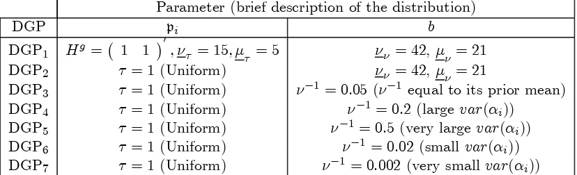
Table 1: SpeciÞcation of the (hyper) parameters for the distributions from which the parameters are drawn in the simulation experiment.
Parameter (brief description of the distribution)
DGP pi b
DGP1 Hg =¡ 1 1 ¢
0
, ντ = 15, µ
τ = 5 νν = 42,µν = 21
DGP2 τ = 1(Uniform) νν = 42,µν = 21
DGP3 τ = 1(Uniform) ν−1 = 0.05 (ν−1 equal to its prior mean) DGP4 τ = 1(Uniform) ν−1 = 0.2 (largevar(αi))
DGP5 τ = 1(Uniform) ν−1 = 0.5 (very largevar(αi))
DGP6 τ = 1(Uniform) ν−1= 0.02 (small var(αi))
DGP7 τ = 1(Uniform) ν−1= 0.002(very small var(αi))
testing ideas underlying frequentist econometrics (e.g. the idea of null hypothesis and the importance allocated to frequentist concepts such as the size of a test). However, as argued in Selke, Bayarri, and Berger (2001) and Berger and Selke (1987), the ideas underlying Bayesian model comparison are very different. Accordingly, following their arguments, in our simulation experiment we repeatedly draw data sets from different distributions. In particular, we set up distributions over our model space and parameter spaces and draw from these. For each draw of a model and parameter values, we then draw an artiÞcial data set. All our DGPs involve the same distributions over the model space and, accordingly, each of our seven DGPs arise from different distributions over the parameters. Note that these distributions have the same functional form as our priors, but the hyperparameters selected to create our DGPs do not have to coincide with the prior hyperparameters we use to estimate our models.
To be precise, in each of our DGPs data is drawn from each model with probability 1/4, which is equal to the prior probability of each model. Conditional on model Mi, the parameters are drawn
from distributions that are of the same form as the prior, but with different hyperparameters. In all cases we use ρb = 0.4. The speciÞcation of the remaining hyperparameter values for each of these distributions is given in Table 1.
Note that DGP1 involves the same informative distribution over the cointegrating space as we use in our prior, but the remaining DGPs are less informative. For the remaining parameters, we have a wide variety of speciÞcations. The speciÞcations in each DGP imply we draw Ai (deÞned in (4))
from a Uniform distribution on the Stiefel manifold. For DGP2 to DGP7 weÞx τ equal to 1, which implies that βi is also drawn from a Uniform distribution. This contrasts with the prior we use for pi =sp(βi), which gives more weight to the space deÞned byH. In addition, DGP3 to DGP7 vary in the expected value ofκi. Higher values ofν−1 imply higher expected values forκiand therefore higher
expected values for the singular values ofΠi. Note that there is 95% prior probability thatν−1 lies in
For each DGP, 2500 artiÞcial data sets were generated. For each data set, the posterior probability of each model (i.e. each rank combination) was calculated. In order to analyse the performance of posterior probabilities in this setup, let us deÞne the following concepts (see Selke, Bayarri, and Berger, 2001, for the development of these concepts). Let Ci(0.5)be the set of data sets in which model Mi
had posterior probability higher than 0.5. Assume that a model is selected whenever its posterior probability is higher than 0.5 and letRi(0.5)be deÞned as an error rate that gives the proportion of
the samples inCi(0.5)that werenot generated from modelMi.
To motivate why these are interesting metrics, we digress brießy to provide a bit of the theory from Selke, Bayarri and Bayarri (2001). Consider the ideal case where the distribution used to generate the datasets is the same as the prior. For this case, suppose Mi is chosen whenever its posterior model
probability (pi) is equal to a particular valuep∗i. From the deÞnition of posterior model probability,
the error rate that results (i.e. the proportion of samples that were classiÞed as Mi but were in fact
generated from another model) is equal to1−p∗i. Thus, posterior model probabilities, unlikep-values, are constructed to reßect true error rates (see also Berger and Selke, 1987, for discussion). However, it is unlikely that we will ever simulate a dataset that results in posterior probability ofMi beingexactly
p∗i so this approach is hard to implement. Therefore, one possibility would be to accept those draws with posterior model probability lying in the interval(p∗i −ε, p∗i +ε), whereεis a small number. This is what Selke, Bayarri and Berger (2001) do. Alternatively, a simple rule of thumb such as "selectMi
if pi > p∗i" can be used (as we have done with pi∗ = 0.5) and the average value of pi (pi) among the
datasets in Ci(0.5)can be reported and the previous reasoning implies this will also be informative
about the error rateRi(0.5). In particular, if the number of datasets is large and are generated from
the prior, Ri(0.5)will be equal to 1−pi.
Table 2 shows the values of pi, Ri(0.5) and the number of data sets in Ci(0.5). Overall, the
strategy of choosing Mi when pi >0.5 seems to work very well, selecting the correct model much of
the time. Recall thatDGP1draws all model parameters, except forΣ, from the prior. Not surprisingly, therefore, Table 2 shows that for DGP1,Ri(0.5)is very close to(1−pi) for everyi= 1, ...,4. These
two quantities are still close for every i for DGP2 and DGP3, which indicates that posterior model probabilities are still a reliable measure of error when the prior of βi is misspeciÞed and/or ν−1 is Þxed to a particular value instead of being random. When ν−1 = 0.2 (DGP
4), which is far outside the prior 95% credible interval of (0.032, 0.077), (1−pi) is still close toRi(0.5)for everyi. Similarly,
whenν−1 = 0.02(DGP
6), which is small compared to prior information, posterior model probabilities continue to be a reliable measure of error for every i. However, when ν−1 = 0.5 (DGP5), posterior model probabilities are not reliable when modelM4 is chosen ((1−pi) < Ri(0.5)), although they still
seem to be reasonable when models M1 to M3 are selected. Something similar, but in the opposite direction, happens when ν−1 is very small (DGP7). In this case, the posterior model probability is only a reliable measure of error whenM4 is chosen.
In our case, for example, it should be noted that DGP5 tends to generate very explosive processes whenever ri = 1, resulting in data that would be extremely unreasonable (at least for standard
ap-plications with macroeconomic data such as the one considered in the next section). For example, it can be shown that DGP5 implies that about 45% of the datasets would have (|y1,t|>1000) for every t= 1, .., T whenr1=r2 = 1, which is not sensible for macroeconomic data such as that which we use in our application.
M1 M2 M3 M4 DGP1 Ri(0.5) 0.07 0.05 0.06 0.03
1−pi 0.06 0.05 0.05 0.02
f
Ni 842 527 545 330
DGP2 Ri(0.5) 0.05 0.03 0.04 0.03
1−pi 0.05 0.04 0.05 0.02
f
Ni 844 541 519 344
DGP3 Ri(0.5) 0.04 0.05 0.03 0.03
1−pi 0.05 0.04 0.04 0.02
f
Ni 830 545 518 354
DGP4 Ri(0.5) 0.01 0.03 0.07 0.09
1−pi 0.07 0.04 0.05 0.03
f
Ni 855 540 531 307
DGP5 Ri(0.5) 0.004 0.105 0.107 0.255
1−pi 0.079 0.067 0.061 0.046
f
Ni 765 531 542 392
DGP6 Ri(0.5) 0.11 0.06 0.07 0.02
1−pi 0.06 0.05 0.05 0.03
f
Ni 840 558 498 341
DGP7 Ri(0.5) 0.36 0.22 0.24 0.05
1−pi 0.10 0.10 0.10 0.07
f
[image:20.595.194.431.197.515.2]Ni 868 514 542 289
Table 2: Error rates (Ri(0.5)), one minus the average posterior probabilities (1−pi) and number of
samples inCi(0.5)(Nfi) for eachDGP.
Table 3 shows other measures that illustrate the performance of Bayesian model selection in this context. For each DGP and model from which the data was generated, it gives the proportion of times (denoted %i) that model Mi had the largest posterior probability. In addition, it shows the average posterior model probability (denotedPi) ofMifor each DGP and each generating model. Note that the proportion of times that the correct model has largest posterior model probability is almost always near or above 90%, and that on average posterior model probabilities are accordingly large. The exception is DGP7, where the detection rate of the true model is lower, as are average posterior model
be more similar to data generated when r= 0, and hence model selection becomes more difficult and we see slightly larger values of %1 and P1.
%1 %2 %3 %4 P1 P2 P3 P4
DGP1 M1 0.99 0.00 0.01 0.00 0.94 0.03 0.03 0.00 M2 0.05 0.94 0.01 0.01 0.05 0.91 0.01 0.03 M3 0.05 0.00 0.94 0.01 0.05 0.00 0.91 0.04 M4 0.03 0.07 0.07 0.84 0.02 0.06 0.07 0.84
DGP2 M1 0.99 0.00 0.00 0.00 0.94 0.03 0.03 0.00 M2 0.04 0.95 0.00 0.01 0.04 0.92 0.00 0.03 M3 0.03 0.00 0.95 0.01 0.04 0.00 0.92 0.04 M4 0.01 0.03 0.04 0.92 0.01 0.03 0.05 0.91 DGP3 M1 0.98 0.01 0.00 0.00 0.94 0.03 0.03 0.00
M2 0.03 0.96 0.00 0.01 0.03 0.93 0.00 0.04 M3 0.03 0.00 0.96 0.01 0.03 0.00 0.93 0.03 M4 0.00 0.04 0.04 0.92 0.00 0.04 0.04 0.91 DGP4 M1 0.95 0.02 0.03 0.00 0.90 0.05 0.05 0.00
M2 0.01 0.96 0.00 0.03 0.01 0.94 0.00 0.05 M3 0.01 0.00 0.97 0.02 0.01 0.00 0.94 0.06 M4 0.01 0.01 0.04 0.94 0.01 0.01 0.04 0.94 DGP5 M1 0.85 0.07 0.06 0.02 0.79 0.08 0.09 0.03
M2 0.00 0.93 0.00 0.06 0.00 0.90 0.00 0.10 M3 0.00 0.00 0.91 0.08 0.00 0.00 0.88 0.11 M4 0.00 0.00 0.01 0.99 0.00 0.00 0.01 0.99 DGP6 M1 0.98 0.01 0.01 0.00 0.94 0.03 0.03 0.00
M2 0.07 0.92 0.00 0.01 0.07 0.89 0.01 0.04 M3 0.09 0.01 0.90 0.01 0.08 0.01 0.87 0.04 M4 0.03 0.07 0.08 0.82 0.03 0.07 0.08 0.82 DGP7 M1 0.98 0.01 0.01 0.00 0.91 0.04 0.04 0.00
[image:21.595.139.490.116.523.2]M2 0.24 0.73 0.02 0.01 0.21 0.70 0.03 0.05 M3 0.23 0.02 0.74 0.01 0.22 0.03 0.70 0.05 M4 0.10 0.19 0.21 0.49 0.09 0.19 0.20 0.51
Table 3: Two summaries (%i andPi) for each DGP.%i is the percentage of times thatMi has largest
posterior model probability. Pi is the average posterior model probability of Mi.
4
Empirical Work
In this section we investigate support for the monetary model of the exchange rate commonly employed in international Þnance. We focus upon the speciÞcation proposed by Groen (2000) which implies a particular testable relationship among the following variables: ei,t, the log of the exchange rate for countryiat timet;mi,t, the log of the ratio of the quantity of domestic to foreign money supply; and
exchange rates, the theory implies the relation
ei,t−β1mi,t−β2xi,t=β0+zi,t
will be stationary (i.e., zi,t should be an I(0) process) with β1 = 1 and β2 <0. If the variables in the
vectoryi,t= (ei,t, mi,t, xi,t) areI(1), this model implies they cointegrate with a particular cointegrating space. The data are quarterly and consist of U.S. dollar exchange rates and the log ratio of money (m) and income (x) for France (i= 1), Germany (i= 2), and the United Kingdom (i= 3) to the U.S. equivalents. The dat runs from the Þrst quarter of 1973 to the last quarter of 1994. The data were those used in Groen and Kleibergen (2003) and are described in detail in Groen (2000).
We have chosen this application because the economic model implies a varied and clear set of testable restrictions on the cointegrating space. That is, we have a requirement that the cointegrating rank be one for all countries, a linear restriction on β1, as well as an inequality restriction upon
β2. We note that it is often the case that the economic model of interest implies such a set of joint
restrictions, some of which are linear and some are nonlinear. In such a case, classical inference usually proceeds with a mixture of sequential testing and informal inference to gather evidence for or against the model, with no single statistic with known power to indicate the degree of support in favor of the model. Therefore, the classical work of Groen, which tested sequentially the rank restriction and the other restrictions, provided only informal evidence about the degree of support for the model. An advantage of using the Bayesian approach is that we are able to provide a formal summary of the evidence for the model via posterior model probabilities. We are also able to assess the evidence, if desired, for components of the model. For example, we may be interested in whether the variables cointegrate or whether the cointegrating ranks are common to all countries, or whether the β0s are
common across all countries.
Within the speciÞcation of the statistical model we use, the monetary exchange rate model implies thatri= 1for each country and that the cointegrating spaces are restricted. In particular, if we deÞne the orthogonal matrixH as:
H=
⎡ ⎢ ⎣
1 √
2 0
−√1 2 0
0 1
⎤ ⎥ ⎦ ,
and introduce the semi-orthogonal vectorϕi=
ϕ1,i
ϕ2,i
, we can write these restrictions as:
βi=Hϕi=
⎡ ⎢ ⎣
1 √2ϕ1,i
−√1 2ϕ1,i
ϕ2,i
⎤ ⎥
⎦, with ϕ2,i
ϕ1,i
>0. (22)
equality of the ranks for all panels (ri =r for all i), and equality of the cointegrating spaces for all panels, pi=psuch thatri=r and βi=β for all i.
We compute posterior probabilities distributions for the cointegrating ranks from both unrestricted and restricted models. We consider two types of restrictions. The Þrst imposes the same unknown cointegrating space: βi=β and ri=r for all i. The second restricts the cointegrating space of at least one country, such that sp(βi)⊆ sp(H) for some i with ri = 1,21 0. This makes a total of 221 models. Following Groen and Kleibergen (2003), all models include an intercept and 3 seasonal dummies and weÞx the number of lags equal to 3. As in the artiÞcial data experiment in the previous section, we choose our prior hyperparameters as: νν = 42, µν = 21, ντ = 15, µτ = 5, and ρb = 0.4. We use 15000 replications of the sampling algorithm presented in Section 2.3. For the sake of comparison, we also calculate the Bayesian Information Criterion (BIC) for each of these models1 1.
Recall we let i= 1,2,3 correspond to France, Germany and UK, respectively. The BIC selects the model with (r1 =r2 =r3 = 0) as the best model, followed by the model with (r1 = 1, r2 =r3 = 0) and
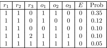
no other restrictions. If posterior model probabilities are calculated using the BIC approximation, these two models would get 90% of the probability. However, the actual posterior model probabilities calculated using our approach are spread over a wide range of models: no less than 28 models would be required to contain 98% of the probability. Table 4 presents the details of the 5 most likely models, which get 71.4% of the probability mass. All these models assign rank equal to one to France and Germany and restrictsp(βi)⊆sp(H) in at least one country. In particular, the model withri= 1and
sp(βi)⊆sp(H) for every i, which gives support to the monetary exchange model, has a non negligible probability that is equal to 0.05. Conditional on this model,P r(φ2i/φ1i>0for i= 1,2,3)1 2= 0.12, which means that the probability of all the restrictions implied by the the monetary exchange model holding in every country is 0.12∗0.05 = 0.006. The probability of many other restrictions of interest can be evaluated by simply adding up the posterior model probabilities of models in which the restriction is true. For example, P r(r1 = r2 = r3) = 0.09, P r(sp(β1) = sp(β2) = sp(β3)) = 0.004, P r(r2 = 1) = 0.86,
P r(sp(β1) ⊆sp(H), r1 >0) = 0.79. Finally, the probability that (sp(βi) ⊂sp(H), ri = 1) for at least one country is 0.94, which again gives support to the monetary exchange model holding in at least one country.
1 0
Ifri= 1,thenpi⊂pH, while ifri= 2,thenpi=pH.
1 1In order to calculate the penalty for the number of parameters in the BIC, we count the parameters in the
semi-orthogonal but otherwise unrestricted βi matrix as nri−r2i, which is the dimension of the Grassman manifold Gn,ri deÞned above (Strachan and Inder, 2004). Similarly, when βi is restricted such that pi ⊆ pH, we Þx the penalty
corresponding to the semi-orthogonal but otherwise unrestricted φi matrix to be 2ri−r2i. We use our algorithm to
search for the maximum value of the actual likelihood by using 1000 draws from a modiÞed posterior density. This modiÞcation increases the accuracy of the obtained maximum likelihood values and consists in analysing the posterior that results when the sample size is increased by a factor of 600 and the additional data is just a replication of the real data. Therefore, the maximum value of the log likelihood function in this modiÞed dataset is 600 times the value of the log likelihood in our real data. And most importantly, the dispersion of the posterior around the mode will be much smaller and therefore the accuracy of the maximized likelihood will be much larger.
1 2This probability was approximated by the proportion of draws from the posterior of this model in which the restriction
r1 r2 r3 o1 o2 o3 E Prob
1 1 0 1 1 0 0 0.35
1 1 0 1 0 0 0 0.12
1 1 0 0 1 0 0 0.10
1 1 2 1 1 1 0 0.10
[image:24.595.220.407.78.163.2]1 1 1 1 1 1 0 0.05
Table 4: Posterior probabilities for the 5 most likely models. TheÞrst 3 columns indicate the rank of each country in a particular model. i= 1,2,3 corresponds to France, Germany and UK, respectively. In the following three columnsoi takes value1when the restrictionsp(βi)⊆sp(H) is imposed and0
otherwise. E takes value 1 if the restrictionsp(β1) =sp(β2) =sp(β3)is imposed and zero otherwise. The last column indicates the probability of each model.
5
Conclusion
In this paper, we have discussed Bayesian inference in cointegrated panel data models. We adopt a very general speciÞcation where each individual is characterized by its own vector error correction model. Special cases of this model allow for individuals to have common cointegrating rank and/or common cointegrating spaces. We develop a noninformative prior as well as an informative prior which allows for sensible priors on the cointegration spaces. The latter prior also allows for prior information about the degree of common structure across individuals to be used. Efficient posterior simulation is carried out using a collapsed Gibbs sampler.
While we consider this a useful start to employing Bayesian methods in this area of models, there are a number of directions for future development. For instance, in a PPP study, Li (1999) argues that estimating relationships of interest individually for each country results in overly noisy estimates. On the other hand, imposing strict homogeneity by assuming these relationships are the same for all countries tends to be overly severe due to the differences in macroeconomic policies in each country. Such severe restriction are often rejected. Li suggests specifying an unknown hierarchical prior and conducting inference upon the distribution from which the parameters for the PPP relations come, not upon the actual PPP parameters themselves. In this paper we have assumed that the cointegrating spaces came from a common known prior distribution and investigated support for common cointegrating spaces (pi=pfor alli). To adopt the Li approach, a hierarchical prior could be placed upon the prior distribution for the cointegrating spaces, rather than assuming a known prior distribution. That is, a prior could be placed uponpH in Section 2.2.2.