MINIMUM ENTROPY RESTORATION USING FPGAS AND HIGH-LEVEL
TECHNIQUES
Robin Bruce
1, Caroline Ruet
2, Stephen Marshall
3, Malachy Devlin
41Institute for System Level Integration, Livingston, Scotland, EH54 7EG, phone: +44-117-377-7144, email: [email protected], web:www.sli-institute.ac.uk 2
Institut National des Sciences Appliquées, Rennes, France, 3Image Processing Group, Uni. of Strathclyde, Glasgow, Scotland, 4
Nallatech Ltd., Cumbernauld, Scotland
ABSTRACT
One of the greatest perceived barriers to the widespread use of FPGAs in image processing is the difficulty for application specialists of developing algorithms on reconfigurable hard-ware. Minimum entropy deconvolution (MED) techniques have been shown to be effective in the restoration of star-field images. This paper reports on an attempt to implement a MED algorithm using simulated annealing, first on a micro-processor, then on an FPGA. The FPGA implementation uses DIME-C, a C-to-gates compiler, coupled with a low-level core library to simplify the design task. Analysis of the C code and output from the DIME-C compiler guided the code optimisation. The paper reports on the design effort that this entailed and the resultant performance improvements.
1. INTRODUCTION
Research into the use of field-programmable gate arrays (FPGAs) in image processing began in earnest at the begin-ning of the 1990s. Since then, many thousands of publica-tions have pointed to the computational capabilities of FPGAs. During this time, FPGAs have seen the application space to which they are applicable grow in tandem with their logic densities. Reference [1] is a good introduction to FPGA-based reconfigurable computing in general, and [2] describes well the issues surrounding FPGA-based image processing. When investigating a particular application, re-searchers compare FPGAs with alternative technologies such as Digital Signal Processors (DSPs), Application-Specific Integrated Circuits (ASICs), microprocessors and vector processors. The metrics for comparison depend on the needs of the application, and include such measurements as raw performance, power consumption, unit cost, board footprint, non-recurring engineering cost, design time and design cost. The key metrics for a particular application may also include ratios of these metrics, e.g. power/performance, or performance/unit-cost. The work detailed in this paper compares a 90nm-process commodity microprocessor with a platform based around a 90nm-process FPGA, focussing on design time and raw performance.
The application chosen for implementation was a minimum entropy restoration of star-field images with simulated an-nealing used to converge towards the globally-optimum solu-tion. The authors did not choose this application in the belief
that it would particularly suit one technology over another, but instead selected it as being representative of a computa-tionally intensive image-processing application.
2. MINIMUM ENTROPY DECONVOLUTION
Image restoration using the minimum entropy deconvolution (MED) method is discussed at length in [3]-[8]. However, the algorithm presented in [3] does not offer a precise and clear explanation of the different stages. While the principle is very clearly defined, the different steps of the algorithm are confusing. To implement this algorithm in software and on an FPGA, it is important to understand the complex cal-culations in order to optimise them. The purpose of this sec-tion is then not to redefine the basis of the MED optimisa-tion but to explain with more accuracy the different stages of the simulated annealing algorithm used in this application.
2.1 Simulated Annealing method
Suppose the image distortion system can be modelled as:
) , ( ) , ( ) , ( ) ,
(k1 k2 xk1 k2 hk1 k2 k1 k2
y = ∗ +ξ . (1)
What is desired is an estimate of the original image x(k1,k2) from the observed image y(k1,k2), assuming that the image was distorted by a blurring system whose point spread func-tion (PSF) can be approximated by a Gaussian funcfunc-tion:
) , 0 [
, 0
2 , 1 , 0 , 1 , 2 2 , 1 ,
exp ) (
2 2 2 1
∞ ∈
− − =
+
− =
d
otherwise
m m for d
m m d
h γ . (2)
where m1, m2 designates the size of the PSF (m1, m2 = -2, -1, 0, 1, 2 for a 5 x 5 filter) and γ is a constant used to normalise the Gaussian function. d corresponds to the width of the PSF and determines the blurring level applied to the image. ξ(k1,k2) is an additive white Gaussian noise defined by a mean and a variance.
[
]
∑∑
∑∑
∑∑
− ∗ + = 1 2 1 2 1 2 2 2 1 2 1 2 1 2 1 4 2 2 1 2 ) , ( ) , ( ) , ( ) , ( ) , ( )) ( , ( k k k k k k k k y k k h k k x k k x k k x d h x E λ . (3)The first estimation for x can be chosen to be either the ob-served image y(k1,k2), an empty image or a random image. SA differs from other iterative techniques in that it uses a temperature parameter to avoid getting trapped in a local optimum, something which is generally the case in other methods, such as gradient descent.
In each iteration of the algorithm, a new candidate for the estimate of the original image is computed. Also, a variation in the PSF is produced by varying the parameter blurring level coefficient d. These slight changes result in the system energy E changing by ∆E. If ∆E is negative the adjustments to the image x(k1,k2) and the parameter d are accepted. If ∆E is positive or zero the adjustments of the image x(k1,k2) and the parameter d are accepted with a probability which de-creases exponentially with ∆E/T. At the beginning of the process, the temperature T is large and therefore the adjust-ments are more likely to be accepted, allowing gross fea-tures of the image to appear. At low temperature levels, the algorithm is more likely to reject image adjustments, allow-ing only fine adjustments to the estimated image. When the temperature becomes zero, the procedure stops at the opti-mal state of minimum energy.
2.2 Algorithm steps
At this point, we use x and y as shorthand for x(k1,k2), y(k1,k2) respectively to simplify the explanatory text.
• Step 0: Set p=0 and initialise α, β, λ, Tp, dp and xp. x0 can be either the observed image, an empty image or even a random image.
T0 is set high. The best way to determine a suitable starting temperature is to run the algorithm and note whether or not adjustments are accepted in a good proportion. (100 can be used as a starting point).
d0 could have a range of [0, ∞] though too large a value would cause the algorithm to fail, the image being too blurred. A range of [0, 20] is therefore more realistic to consider as it gives a PSF that is not too large.
α & λ can be set to 1 to make them neither too small nor too large. However, β has to be very small, 0.0001 being a suitable value.
• Step 1: Compute the energy Ep(xp, h(dp)).
Use (3). Replace x by xp. Replace h(d) by h(dp). This means that the Gaussian function has to be determined for each d. Take y as the observed image.
• Step 2: Select a candidate solution.
Compute the candidate image x’ and the candidate parameter for the Gaussian function d’:
) , ( ' 2 1 1 n n x E x x p p p ∂ ∂ − =
+ α . (4)
p p p d E d d ∂ ∂ − =
+1 β
' . (5)
where ) , ( ) , ( ) , ( ) , ( 2 ) , ( ) , ( ) , ( 1 ) , ( ) , ( ) , ( 4 ) , ( 2 2 1 1 2 1 2 1 2 2 1 1 2 1 4 2 1 2 2 1 2 2 1 4 2 1 2 2 1 2 1
1 2 1 2 1 2 1 2 1 2 1 2 n k n k h k k y m m h m k m k x k k x k k x n n x k k x k k x n n x n n x E p
k k m m p p k k p k k p p k k p k k p p p − − ⋅ − ⋅ − − + − ⋅ = ∂ ∂
∑∑∑∑
∑∑
∑∑
∑∑
∑∑
λ. (6)
k1 & k2 span the entire image and m1 & m2 give the size of the Gaussian function. n1 & n2 are used to define a particular pixel of the considered image xp. The computation of ∆xp is carried out for every pixel of the image to get an overall new value of this image. This value must be computed n2 times for an image of size n x n.
and:
∑∑
∑∑∑∑
⋅ − − + ⋅ − ⋅ − − = ∂ ∂ 1 2 1 2 1 2) , ( ) , ( ) ( ) , ( ) , ( ) , ( 2 2 1 2 2 1 1 2 2 2 2 1 2 1 2 1 2 2 1 1 m m p p p k k m m p
p p m m h m k m k x d m m k k y m m h m k m k x d E λ . (7)
k1, k2, m1 and m2 have the same definition as before. This computation is unique for each iteration of the algorithm.
• Step 3: Compute the energy E’p+1(x’p+1, h(d’p+1)). Let: p
p E
E
E= −
∆ ' +1 . (8)
• Step 4: If:
r T E p > ∆ −
exp . (9)
Then: p p p p p
p x d d and T T
x +1= ' +1, +1= ' +1 +1= . (11) where r is a random number on the interval [0,1].
Else:
) (
, 1 1
1 p p p p p
p x d d and T f T
x + = + = + = . (12)
• Step 5: p=p+1.
If the temperature T is not zero, the termination condition is not satisfied, go to Step 1.
• Step 6: Output xp+1 is the estimation image. The last xp+1 image is the estimate of the original image.
The data used in calculations in the algorithm begin as 8-bit integer pixel values. The 24 bits of precision of IEEE754 single precision suffices for all the calculations in the algo-rithm. Floating-point calculations are required because there are parts of the algorithm that require higher dynamic range than provided by integer arithmetic. The dynamic range re-quirements are fully satisfied by single precision, so there is no requirement for double-precision calculations. Nallatech‘s DIME-C compiler, a C-to-Gates compiler that targets FPGA computing boards was used. The compiler is well-suited to floating-point computation, uses a subset of ANSI C and allows for the inclusion of libraries of low-level functional cores.
3. HIGH-LEVEL TECHNIQUES FOR FPGAS
3.1 Traditional FPGA Programming
Field-Programmable Gate Arrays are programmed by means of a bitstream or bitfile that tells the chip how to configure its internal logic, memory and routing resources. Without this bitstream the chip has no functionality at all. The “tradi-tional” method of obtaining an FPGA bitstream is to de-scribe the desired system in terms of synchronous electronic components using a hardware description language (HDL). The most well-known of these HDLs are VHDL and Ver-ilog. To go from a functional specification to a functioning bitstream involves writing HDL, then simulating it. Due to the low level description and verbose nature of these HDL languages this can be a lengthy and error-prone process us-ing expensive tools. Once the HDL is functionus-ing correctly in simulation, it is passed through synthesis tools. For high-performance computing applications, this “traditional” proc-ess may result in good performance and low resource use, but it requires an expertise that most application developers do not possess and requires an investment of time that would be unreasonable for most applications.
3.2 High-Level FPGA Programming
There has been a concerted research effort aimed at develop-ing design techniques for reconfigurable computdevelop-ing that bet-ter suit application-domain specialists [9]-[11]. Among the high-level tools that promise to simplify the task of imple-menting an algorithm is DIME-C. DIME-C is a compiler that turns high-level code into a combination of VHDL and pre-synthesized logical netlists. The C that DIME-C can compile is a subset of ANSI C. This means that while not everything that can be compiled using a standard C compiler can be compiled by DIME-C, all source code that can be compiled in DIME-C can also be compiled using a standard C com-piler. This allows for rapid functional verification of algo-rithm code before compilation to FPGA hardware.
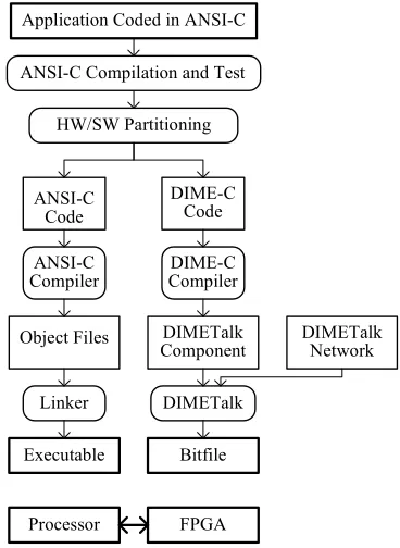
Application developers write code as standard ANSI C, avoiding certain constructs such as pointers. The compiler aims to extract obvious parallelism within loop bodies as well as to pipeline loops wherever possible. In nested loops, the compiler pipelines the innermost loop. One must also ensure loops do not break any of the rules for pipelining. The code must be non-recursive, and must not access memory arrays more times per cycle than can be accommodated by the underlying memory structure. Beyond these considera-tions the user does not need any knowledge of hardware de-sign in order to produce VHDL code of pipelined architec-tures that implement algorithms. DIME-C supports bit-level, integer and floating-point arithmetic. The compiler also sup-ports the inclusion of support libraries that allow users to implement functions previously created either in DIME-C or via a more traditional design process directly using HDLs. Additionally, the compiler seeks to exploit the essentially serial nature of the programs to resource share between sec-tions of the code that do not execute concurrently. This means the compiler can implement complex algorithms that demand many floating-point operations, provided no concur-rently executing code aims to use more resources than are available on the device. Such a resource-sharing optimisation would be extremely difficult to implement manually using HDL. The compiler displays its temporal scheduling visually and produces a report file that together show the parallelisa-tion of the user code. Figure 1 below shows the programming process used. DIMETalk is used here is equivalent to a soft-ware linker to link the DIME-C code to the necessary mem-ory structure and the specific hardware platform.
Application Coded in ANSI-C
ANSI-C Compilation and Test
HW/SW Partitioning
ANSI-C Code
DIME-C Code
DIME-C Compiler ANSI-C
Compiler
Object Files DIMETalk Component
DIMETalk Network
Linker DIMETalk
Executable Bitfile
[image:3.612.334.518.413.665.2]Processor FPGA
3.3 Core Libraries
DIME-C allows for the inclusion of core libraries. Core li-braries allow users to use FPGA functions that have been developed, tested and packaged. Reference [12] gives detail on the motivations for integrating core libraries into high-level tools. The reference also discusses the creation of a math library that is used in the context of this project. This math library has been created using standard HDL tech-niques, then packaged in such a way as to be indistinguish-able from the math library used in ANSI C to the tools user. The exponential function and a pseudo-random number gen-erator function are used in the simulated annealing algorithm that is implemented here. These functions were created in VHDL, then packaged into a core library to allow them to be called in an identical manner to their ANSI C counterparts. Without access to this math library, the implementation of the simulated annealing algorithm would have represented a far more significant research challenge. This paper is, believed to be, the first publication on the use of this mathematical core library in an actual application.
The difference between the use of library-enabled high-level FPGA languages such as DIME-C and a traditional HDL approach is marked. It is analogous to the difference between programming in the C language with access to function li-braries and creating programs in assembler without any sup-port libraries.
4. IMPLEMENTATION
Two of the authors involved in the work took the role of application specialists, in that they focussed primarily on developing the image processing application and obtaining a working software implementation. The other two authors were reconfigurable-computing specialists, who looked to interact with the application specialists to help them make the transition to a hardware implementation, instructing them on how to get the most from the design tools used.
4.1 Software and Hardware Platforms
The software platform was a 3.2 GHz Intel Pentium D proc-essor with 2 GB of DRAM, with the GNU C compiler, ver-sion 3.4.2. The targeted FPGA platform was a Nallatech PCIXM card, with the DIME-C compiler. The H101-PCIXM card has a Xilinx Virtex-4 LX100 FPGA, 512 MB of DRAM and 4 banks of 200MHz, 4 MB SRAM.
4.2 ANSI C Software Implementation
In the first stage of implementation, the application special-ists developed the algorithm from theory to implementation in ANSI C on a commodity microprocessor. This stage rep-resented the majority of the time spent in the project, around 100 person-hours. The application specialists carried out this work without any significant input from the reconfigurable-computing specialists. Once the algorithm was functioning satisfactorily in software, the second stage began.
4.3 DIME-C Hardware Implementation
In the second stage of the algorithm, the application special-ists and the reconfigurable computing specialspecial-ists worked together to optimise the algorithm, to migrate it to the DIME-C environment, and to characterise its performance. This process took approximately 25 person-hours. The ANSI C implementation was optimised for performance in order to make for the fairest comparison. The software performance was improved by several orders of magnitude during this time; otherwise, the software-hardware comparison would have been more weighted in favour of the FPGA.
A typical procedure for the porting of algorithms to software is to first profile the software-implemented algorithm, then implement on the FPGA the functions that represent the ma-jority of the calculation time. There are disadvantages to this approach. It neglects to take into account the data transfers that are necessary between the reconfigurable computing platform and the microprocessor-based system before and after each function call. When factored in, these data trans-fers can negate any performance improvement in the hard-ware-implemented function. The approach taken here was to implement the entire algorithm on the FPGA, so that the data transfer time is negligible in comparison to the compute time. This means that all improvements to the computation time of a section of the algorithm translate into a measured perform-ance improvement.
4.3.1 Implementation Process
The implementation process consisted of the following steps: 1. Create a DIME-C project using the original source
from the ANSI C project.
2. Adapt the source to allow compilation in both DIME-C and ANSI C environments.
3. Take advantage of the most obvious pipelining op-portunities to create 1st FPGA implementation. 4. Examine the source code and the output of
DIME-C, create an equation that expressed the runtime of the algorithm in cycles, as a function of the parame-ters of the algorithm, divided into key sections. 5. Determine for a typical set of algorithm parameters
the section that takes up the majority of the runtime, and optimise the DIME-C for this section to create the 2nd FPGA implementation.
6. Repeat sections 4&5 to produce the 3rd & 4th FPGA implementations.
4.3.2 Algorithm Performance Characterisation
of the various loops and sections of the code. It is possible to significantly simplify the resultant characteristic expression by factoring out the sections that do not appreciably contrib-ute to the total run time.
The characteristic expression derived for the FPGA-implemented program was as follows:
iter n l c n n Other
l c n n Filter l
c n n Dx De Ncycles
_ ) ) , , , (
) , , , ( )
, , , ( _ (
2 1
2 1 2
1 ⋅ +
+ =
. (13)
Where De_Dx corresponds to equation (6), Filter is the ap-plication of the Gaussian filter to the image and Other is all other operations in the algorithm. n_iter is the number of iterations taken to carry out the simulated annealing algo-rithm. n1 and n2 are the dimensions of the PSF, c and l are the column and line widths of the image respectively. As the Filter section was improved, the performance of the algorithm improved. The evolution of the characteristic equation for Filter through three incarnations of the DIME-C source can be seen below:
) 111 (
2 ) , , , (
) 151 2 3 ( ) 2 ( ) , , , (
) 1 2 ( ) 101 2 ( 3 ) , , , (
2 1 3 _
2 1 2
1 2 _
1 2
2 1 1 _
+ ⋅ ⋅ =
+ ⋅
⋅ =
+ ⋅ ⋅ ⋅ + ⋅ =
l c l c n n Filter
n n l c l c n n Filter
n l c n
l c n n Filter
FPGA FPGA FPGA
. (14)
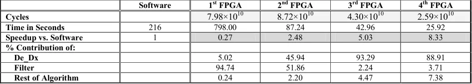
The 4th FPGA implementation improved the performance of De_Dx. De_Dx would remain the focus of a 5th implementa-tion. Table 1 below shows how the four successive imple-mentations of the algorithm on the FPGA platform compared with the optimised microprocessor implementation. Data transfer times were negligible and did not contribute to the result. The results below are for an image of size 800×600, with a 5×5 PSF. The algorithm took 100 iterations to com-plete and the FPGA clock rate was 100MHz.
5. CONCLUSIONS
Latest generation reconfigurable computing platforms are suitable for the implementation of entire image processing algorithms that require significant levels of floating point computation. When using high-level languages significant speedup can be measured. Core libraries further simplify the task of implementing algorithms. The design time that was required to port the algorithm was not disproportionate in comparison to the time spent developing and implementing the algorithm. Developing characteristic expressions for the different algorithmic sections aided in identifying the parts of the algorithm that would most benefit from optimisation, hence speeding up the development process.
REFERENCES
[1] J. Villasenor and B. Hutchings, “The flexibility of con-figurable computing”. IEEE Signal Processing Maga-zine, 15, 5, pp. 67-84, 1998.
[2] C. T. Johnston, K. T. Gribbon and D. G. Bailey, “Im-plementing Image Processing Algorithms on FPGAs. Proceedings of the Eleventh Electronics New Zealand Conference, ENZCon’04, 118-123, 2004
[3] Wu H, Barba J, “Minimum entropy restoration of star field images”. Systems, Man and Cybernetics, Part B, IEEE Transactions on, Vol. 28, No. 2., pp. 227-231., 1998.
[4] R.Wiggins, "Minimum entropy deconvolution,'' Geoex-plor, vol. 16, pp. 21–35, Jan. 1978.
[5] D. Donoho, "On minimum entropy deconvolution,'' in Applied Time Analysis, II. New York: Academic, 1981. [6] R. Wiggins, "Entropy guided deconvolution,'' Geophys.,
vol. 50, pp. 2720–2726, Dec. 1985.
[7] M. Ooe, and T. J. Ulrych, "Minimum entropy deconvo-lution with an exponential transformation,'' Geophys. Prosp., vol. 27, pp. 458–473, 1979.
[8] S. Kirkpatrick, C. D. Gelatt, and M. P. Vecchi, "Optimi-sation by simulated annealing,'' Science, vol. 220, pp. 671–680, May 1983.
[9] I. Alston and B. Madahar, “From C to netlists: hardware engineering for software engineers?” Electronics & Communication Engineering Journal, 14, 4, pp. 165-173, 2002.
[10]R. Rinker, J. Hammes, W. A. Najjar, W. Bohm and B. Draper. “Compiling image processing applications to reconfigurable hardware.” Proceedings. IEEE Inter-national Conference on Application-Specific Systems, Architectures, and Processors, Boston, MA, USA, pp. 56-65, 2000
[11] J. Hammes, B. Rinker, W. Bohm, W. Najjar, B. Draper and R. Beveridge. “Cameron: high level language compilation for reconfigurable systems.” Proceed-ings International Conference on Parallel Architectures and Compilation Techniques, Newport Beach, CA,
USA, pp. 236-244, 1999
[image:5.612.71.544.607.692.2][12]R. Bruce, M. Devlin, S. Marshall, “Lessons Learned Implementing the VSIPL API on Reconfigurable Com-puters.” Proceedings of Military and Programmable Logic Devices International Conference, Washington DC, USA, Submission 229, 2006.
Table 1 – Performance Comparison of FPGA implementations versus software
Software 1st FPGA 2nd FPGA 3rd FPGA 4th FPGA
Cycles 7.98×10¹⁰ 8.72×10¹⁰ 4.30×10¹⁰ 2.59×10¹⁰
Time in Seconds 216 798.00 87.24 42.96 25.92
Speedup vs. Software 1 0.27 2.48 5.03 8.33
% Contribution of:
De_Dx 5.02 45.94 93.29 88.91
Filter 94.74 51.86 2.24 3.71
MINIMUM ENTROPY RESTORATION USING FPGAS AND HIGH-LEVEL
TECHNIQUES
Robin Bruce
1, Caroline Ruet
2, Stephen Marshall
3, Malachy Devlin
41Institute for System Level Integration, Livingston, Scotland, EH54 7EG, phone: +44-117-377-7144, email: [email protected], web:www.sli-institute.ac.uk 2
Institut National des Sciences Appliquées, Rennes, France, 3Image Processing Group, Uni. of Strathclyde, Glasgow, Scotland, 4
Nallatech Ltd., Cumbernauld, Scotland
ABSTRACT
One of the greatest perceived barriers to the widespread use of FPGAs in image processing is the difficulty for application specialists of developing algorithms on reconfigurable hard-ware. Minimum entropy deconvolution (MED) techniques have been shown to be effective in the restoration of star-field images. This paper reports on an attempt to implement a MED algorithm using simulated annealing, first on a micro-processor, then on an FPGA. The FPGA implementation uses DIME-C, a C-to-gates compiler, coupled with a low-level core library to simplify the design task. Analysis of the C code and output from the DIME-C compiler guided the code optimisation. The paper reports on the design effort that this entailed and the resultant performance improvements.
1. INTRODUCTION
Research into the use of field-programmable gate arrays (FPGAs) in image processing began in earnest at the begin-ning of the 1990s. Since then, many thousands of publica-tions have pointed to the computational capabilities of FPGAs. During this time, FPGAs have seen the application space to which they are applicable grow in tandem with their logic densities. Reference [1] is a good introduction to FPGA-based reconfigurable computing in general, and [2] describes well the issues surrounding FPGA-based image processing. When investigating a particular application, re-searchers compare FPGAs with alternative technologies such as Digital Signal Processors (DSPs), Application-Specific Integrated Circuits (ASICs), microprocessors and vector processors. The metrics for comparison depend on the needs of the application, and include such measurements as raw performance, power consumption, unit cost, board footprint, non-recurring engineering cost, design time and design cost. The key metrics for a particular application may also include ratios of these metrics, e.g. power/performance, or performance/unit-cost. The work detailed in this paper compares a 90nm-process commodity microprocessor with a platform based around a 90nm-process FPGA, focussing on design time and raw performance.
The application chosen for implementation was a minimum entropy restoration of star-field images with simulated an-nealing used to converge towards the globally-optimum solu-tion. The authors did not choose this application in the belief
that it would particularly suit one technology over another, but instead selected it as being representative of a computa-tionally intensive image-processing application.
2. MINIMUM ENTROPY DECONVOLUTION
Image restoration using the minimum entropy deconvolution (MED) method is discussed at length in [3]-[8]. However, the algorithm presented in [3] does not offer a precise and clear explanation of the different stages. While the principle is very clearly defined, the different steps of the algorithm are confusing. To implement this algorithm in software and on an FPGA, it is important to understand the complex cal-culations in order to optimise them. The purpose of this sec-tion is then not to redefine the basis of the MED optimisa-tion but to explain with more accuracy the different stages of the simulated annealing algorithm used in this application.
2.1 Simulated Annealing method
Suppose the image distortion system can be modelled as:
) , ( ) , ( ) , ( ) ,
(k1 k2 xk1 k2 hk1 k2 k1 k2
y = ∗ +ξ . (1)
What is desired is an estimate of the original image x(k1,k2) from the observed image y(k1,k2), assuming that the image was distorted by a blurring system whose point spread func-tion (PSF) can be approximated by a Gaussian funcfunc-tion:
) , 0 [
, 0
2 , 1 , 0 , 1 , 2 2 , 1 ,
exp ) (
2 2 2 1
∞ ∈
− − =
+
− =
d
otherwise
m m for d
m m d
h γ . (2)
where m1, m2 designates the size of the PSF (m1, m2 = -2, -1, 0, 1, 2 for a 5 x 5 filter) and γ is a constant used to normalise the Gaussian function. d corresponds to the width of the PSF and determines the blurring level applied to the image. ξ(k1,k2) is an additive white Gaussian noise defined by a mean and a variance.
[
]
∑∑
∑∑
∑∑
− ∗ + = 1 2 1 2 1 2 2 2 1 2 1 2 1 2 1 4 2 2 1 2 ) , ( ) , ( ) , ( ) , ( ) , ( )) ( , ( k k k k k k k k y k k h k k x k k x k k x d h x E λ . (3)The first estimation for x can be chosen to be either the ob-served image y(k1,k2), an empty image or a random image. SA differs from other iterative techniques in that it uses a temperature parameter to avoid getting trapped in a local optimum, something which is generally the case in other methods, such as gradient descent.
In each iteration of the algorithm, a new candidate for the estimate of the original image is computed. Also, a variation in the PSF is produced by varying the parameter blurring level coefficient d. These slight changes result in the system energy E changing by ∆E. If ∆E is negative the adjustments to the image x(k1,k2) and the parameter d are accepted. If ∆E is positive or zero the adjustments of the image x(k1,k2) and the parameter d are accepted with a probability which de-creases exponentially with ∆E/T. At the beginning of the process, the temperature T is large and therefore the adjust-ments are more likely to be accepted, allowing gross fea-tures of the image to appear. At low temperature levels, the algorithm is more likely to reject image adjustments, allow-ing only fine adjustments to the estimated image. When the temperature becomes zero, the procedure stops at the opti-mal state of minimum energy.
2.2 Algorithm steps
At this point, we use x and y as shorthand for x(k1,k2), y(k1,k2) respectively to simplify the explanatory text.
• Step 0: Set p=0 and initialise α, β, λ, Tp, dp and xp. x0 can be either the observed image, an empty image or even a random image.
T0 is set high. The best way to determine a suitable starting temperature is to run the algorithm and note whether or not adjustments are accepted in a good proportion. (100 can be used as a starting point).
d0 could have a range of [0, ∞] though too large a value would cause the algorithm to fail, the image being too blurred. A range of [0, 20] is therefore more realistic to consider as it gives a PSF that is not too large.
α & λ can be set to 1 to make them neither too small nor too large. However, β has to be very small, 0.0001 being a suitable value.
• Step 1: Compute the energy Ep(xp, h(dp)).
Use (3). Replace x by xp. Replace h(d) by h(dp). This means that the Gaussian function has to be determined for each d. Take y as the observed image.
• Step 2: Select a candidate solution.
Compute the candidate image x’ and the candidate parameter for the Gaussian function d’:
) , ( ' 2 1 1 n n x E x x p p p ∂ ∂ − =
+ α . (4)
p p p d E d d ∂ ∂ − =
+1 β
' . (5)
where ) , ( ) , ( ) , ( ) , ( 2 ) , ( ) , ( ) , ( 1 ) , ( ) , ( ) , ( 4 ) , ( 2 2 1 1 2 1 2 1 2 2 1 1 2 1 4 2 1 2 2 1 2 2 1 4 2 1 2 2 1 2 1
1 2 1 2 1 2 1 2 1 2 1 2 n k n k h k k y m m h m k m k x k k x k k x n n x k k x k k x n n x n n x E p
k k m m p p k k p k k p p k k p k k p p p − − ⋅ − ⋅ − − + − ⋅ = ∂ ∂
∑∑∑∑
∑∑
∑∑
∑∑
∑∑
λ. (6)
k1 & k2 span the entire image and m1 & m2 give the size of the Gaussian function. n1 & n2 are used to define a particular pixel of the considered image xp. The computation of ∆xp is carried out for every pixel of the image to get an overall new value of this image. This value must be computed n2 times for an image of size n x n.
and:
∑∑
∑∑∑∑
⋅ − − + ⋅ − ⋅ − − = ∂ ∂ 1 2 1 2 1 2) , ( ) , ( ) ( ) , ( ) , ( ) , ( 2 2 1 2 2 1 1 2 2 2 2 1 2 1 2 1 2 2 1 1 m m p p p k k m m p
p p m m h m k m k x d m m k k y m m h m k m k x d E λ . (7)
k1, k2, m1 and m2 have the same definition as before. This computation is unique for each iteration of the algorithm.
• Step 3: Compute the energy E’p+1(x’p+1, h(d’p+1)). Let: p
p E
E
E= −
∆ ' +1 . (8)
• Step 4: If:
r T E p > ∆ −
exp . (9)
Then: p p p p p
p x d d and T T
x +1= ' +1, +1= ' +1 +1= . (11) where r is a random number on the interval [0,1].
Else:
) (
, 1 1
1 p p p p p
p x d d and T f T
x + = + = + = . (12)
• Step 5: p=p+1.
If the temperature T is not zero, the termination condition is not satisfied, go to Step 1.
• Step 6: Output xp+1 is the estimation image. The last xp+1 image is the estimate of the original image.
The data used in calculations in the algorithm begin as 8-bit integer pixel values. The 24 bits of precision of IEEE754 single precision suffices for all the calculations in the algo-rithm. Floating-point calculations are required because there are parts of the algorithm that require higher dynamic range than provided by integer arithmetic. The dynamic range re-quirements are fully satisfied by single precision, so there is no requirement for double-precision calculations. Nallatech‘s DIME-C compiler, a C-to-Gates compiler that targets FPGA computing boards was used. The compiler is well-suited to floating-point computation, uses a subset of ANSI C and allows for the inclusion of libraries of low-level functional cores.
3. HIGH-LEVEL TECHNIQUES FOR FPGAS
3.1 Traditional FPGA Programming
Field-Programmable Gate Arrays are programmed by means of a bitstream or bitfile that tells the chip how to configure its internal logic, memory and routing resources. Without this bitstream the chip has no functionality at all. The “tradi-tional” method of obtaining an FPGA bitstream is to de-scribe the desired system in terms of synchronous electronic components using a hardware description language (HDL). The most well-known of these HDLs are VHDL and Ver-ilog. To go from a functional specification to a functioning bitstream involves writing HDL, then simulating it. Due to the low level description and verbose nature of these HDL languages this can be a lengthy and error-prone process us-ing expensive tools. Once the HDL is functionus-ing correctly in simulation, it is passed through synthesis tools. For high-performance computing applications, this “traditional” proc-ess may result in good performance and low resource use, but it requires an expertise that most application developers do not possess and requires an investment of time that would be unreasonable for most applications.
3.2 High-Level FPGA Programming
There has been a concerted research effort aimed at develop-ing design techniques for reconfigurable computdevelop-ing that bet-ter suit application-domain specialists [9]-[11]. Among the high-level tools that promise to simplify the task of imple-menting an algorithm is DIME-C. DIME-C is a compiler that turns high-level code into a combination of VHDL and pre-synthesized logical netlists. The C that DIME-C can compile is a subset of ANSI C. This means that while not everything that can be compiled using a standard C compiler can be compiled by DIME-C, all source code that can be compiled in DIME-C can also be compiled using a standard C com-piler. This allows for rapid functional verification of algo-rithm code before compilation to FPGA hardware.
Application developers write code as standard ANSI C, avoiding certain constructs such as pointers. The compiler aims to extract obvious parallelism within loop bodies as well as to pipeline loops wherever possible. In nested loops, the compiler pipelines the innermost loop. One must also ensure loops do not break any of the rules for pipelining. The code must be non-recursive, and must not access memory arrays more times per cycle than can be accommodated by the underlying memory structure. Beyond these considera-tions the user does not need any knowledge of hardware de-sign in order to produce VHDL code of pipelined architec-tures that implement algorithms. DIME-C supports bit-level, integer and floating-point arithmetic. The compiler also sup-ports the inclusion of support libraries that allow users to implement functions previously created either in DIME-C or via a more traditional design process directly using HDLs. Additionally, the compiler seeks to exploit the essentially serial nature of the programs to resource share between sec-tions of the code that do not execute concurrently. This means the compiler can implement complex algorithms that demand many floating-point operations, provided no concur-rently executing code aims to use more resources than are available on the device. Such a resource-sharing optimisation would be extremely difficult to implement manually using HDL. The compiler displays its temporal scheduling visually and produces a report file that together show the parallelisa-tion of the user code. Figure 1 below shows the programming process used. DIMETalk is used here is equivalent to a soft-ware linker to link the DIME-C code to the necessary mem-ory structure and the specific hardware platform.
Application Coded in ANSI-C
ANSI-C Compilation and Test
HW/SW Partitioning
ANSI-C Code
DIME-C Code
DIME-C Compiler ANSI-C
Compiler
Object Files DIMETalk Component
DIMETalk Network
Linker DIMETalk
Executable Bitfile
[image:8.612.334.518.413.665.2]Processor FPGA
3.3 Core Libraries
DIME-C allows for the inclusion of core libraries. Core li-braries allow users to use FPGA functions that have been developed, tested and packaged. Reference [12] gives detail on the motivations for integrating core libraries into high-level tools. The reference also discusses the creation of a math library that is used in the context of this project. This math library has been created using standard HDL tech-niques, then packaged in such a way as to be indistinguish-able from the math library used in ANSI C to the tools user. The exponential function and a pseudo-random number gen-erator function are used in the simulated annealing algorithm that is implemented here. These functions were created in VHDL, then packaged into a core library to allow them to be called in an identical manner to their ANSI C counterparts. Without access to this math library, the implementation of the simulated annealing algorithm would have represented a far more significant research challenge. This paper represents the first publication on the use of this mathematical core library in an actual application.
The difference between the use of library-enabled high-level FPGA languages such as DIME-C and a traditional HDL approach is marked. It is analogous to the difference between programming in the C language with access to function li-braries and creating programs in assembler without any sup-port libraries.
4. IMPLEMENTATION
Two of the authors involved in the work took the role of application specialists, in that they focussed primarily on developing the image processing application and obtaining a working software implementation. The other two authors were reconfigurable-computing specialists, who looked to interact with the application specialists to help them make the transition to a hardware implementation, instructing them on how to get the most from the design tools used.
4.1 Software and Hardware Platforms
The software platform was a 3.2 GHz Intel Pentium D proc-essor with 2 GB of DRAM, with the GNU C compiler, ver-sion 3.4.2. The targeted FPGA platform was a Nallatech PCIXM card, with the DIME-C compiler. The H101-PCIXM card has a Xilinx Virtex-4 LX100 FPGA, 512 MB of DRAM and 4 banks of 200MHz, 4 MB SRAM.
4.2 ANSI C Software Implementation
In the first stage of implementation, the application special-ists developed the algorithm from theory to implementation in ANSI C on a commodity microprocessor. This stage rep-resented the majority of the time spent in the project, around 100 person-hours. The application specialists carried out this work without any significant input from the reconfigurable-computing specialists. Once the algorithm was functioning satisfactorily in software, the second stage began.
4.3 DIME-C Hardware Implementation
In the second stage of the algorithm, the application special-ists and the reconfigurable computing specialspecial-ists worked together to optimise the algorithm, to migrate it to the DIME-C environment, and to characterise its performance. This process took approximately 25 person-hours. The ANSI C implementation was optimised for performance in order to make for the fairest comparison. The software performance was improved by several orders of magnitude during this time; otherwise, the software-hardware comparison would have been more weighted in favour of the FPGA.
A typical procedure for the porting of algorithms to software is to first profile the software-implemented algorithm, then implement on the FPGA the functions that represent the ma-jority of the calculation time. There are disadvantages to this approach. It neglects to take into account the data transfers that are necessary between the reconfigurable computing platform and the microprocessor-based system before and after each function call. When factored in, these data trans-fers can negate any performance improvement in the hard-ware-implemented function. The approach taken here was to implement the entire algorithm on the FPGA, so that the data transfer time is negligible in comparison to the compute time. This means that all improvements to the computation time of a section of the algorithm translate into a measured perform-ance improvement.
4.3.1 Implementation Process
The implementation process consisted of the following steps: 1. Create a DIME-C project using the original source
from the ANSI C project.
2. Adapt the source to allow compilation in both DIME-C and ANSI C environments.
3. Take advantage of the most obvious pipelining op-portunities to create 1st FPGA implementation. 4. Examine the source code and the output of
DIME-C, create an equation that expressed the runtime of the algorithm in cycles, as a function of the parame-ters of the algorithm, divided into key sections. 5. Determine for a typical set of algorithm parameters
the section that takes up the majority of the runtime, and optimise the DIME-C for this section to create the 2nd FPGA implementation.
6. Repeat sections 4&5 to produce the 3rd & 4th FPGA implementations.
4.3.2 Algorithm Performance Characterisation
of the various loops and sections of the code. It is possible to significantly simplify the resultant characteristic expression by factoring out the sections that do not appreciably contrib-ute to the total run time.
The characteristic expression derived for the FPGA-implemented program was as follows:
iter n l c n n Other
l c n n Filter l
c n n Dx De Ncycles
_ ) ) , , , (
) , , , ( )
, , , ( _ (
2 1
2 1 2
1 ⋅ +
+ =
. (13)
Where De_Dx corresponds to equation (6), Filter is the ap-plication of the Gaussian filter to the image and Other is all other operations in the algorithm. n_iter is the number of iterations taken to carry out the simulated annealing algo-rithm. n1 and n2 are the dimensions of the PSF, c and l are the column and line widths of the image respectively. As the Filter section was improved, the performance of the algorithm improved. The evolution of the characteristic equation for Filter through three incarnations of the DIME-C source can be seen below:
) 111 (
2 ) , , , (
) 151 2 3 ( ) 2 ( ) , , , (
) 1 2 ( ) 101 2 ( 3 ) , , , (
2 1 3 _
2 1 2
1 2 _
1 2
2 1 1 _
+ ⋅ ⋅ =
+ ⋅
⋅ =
+ ⋅ ⋅ ⋅ + ⋅ =
l c l c n n Filter
n n l c l c n n Filter
n l c n
l c n n Filter
FPGA FPGA FPGA
. (14)
The 4th FPGA implementation improved the performance of De_Dx. De_Dx would remain the focus of a 5th implementa-tion. Table 1 below shows how the four successive imple-mentations of the algorithm on the FPGA platform compared with the optimised microprocessor implementation. Data transfer times were negligible and did not contribute to the result. The results below are for an image of size 800×600, with a 5×5 PSF. The algorithm took 100 iterations to com-plete and the FPGA clock rate was 100MHz.
5. CONCLUSIONS
Latest generation reconfigurable computing platforms are suitable for the implementation of entire image processing algorithms that require significant levels of floating point computation. When using high-level languages significant speedup can be measured. Core libraries further simplify the task of implementing algorithms. The design time that was required to port the algorithm was not disproportionate in comparison to the time spent developing and implementing the algorithm. Developing characteristic expressions for the different algorithmic sections aided in identifying the parts of the algorithm that would most benefit from optimisation, hence speeding up the development process.
REFERENCES
[1] J. Villasenor and B. Hutchings, “The flexibility of con-figurable computing”. IEEE Signal Processing Maga-zine, 15, 5, pp. 67-84, 1998.
[2] C. T. Johnston, K. T. Gribbon and D. G. Bailey, “Im-plementing Image Processing Algorithms on FPGAs. Proceedings of the Eleventh Electronics New Zealand Conference, ENZCon’04, 118-123, 2004
[3] Wu H, Barba J, “Minimum entropy restoration of star field images”. Systems, Man and Cybernetics, Part B, IEEE Transactions on, Vol. 28, No. 2., pp. 227-231., 1998.
[4] R.Wiggins, "Minimum entropy deconvolution,'' Geoex-plor, vol. 16, pp. 21–35, Jan. 1978.
[5] D. Donoho, "On minimum entropy deconvolution,'' in Applied Time Analysis, II. New York: Academic, 1981. [6] R. Wiggins, "Entropy guided deconvolution,'' Geophys.,
vol. 50, pp. 2720–2726, Dec. 1985.
[7] M. Ooe, and T. J. Ulrych, "Minimum entropy deconvo-lution with an exponential transformation,'' Geophys. Prosp., vol. 27, pp. 458–473, 1979.
[8] S. Kirkpatrick, C. D. Gelatt, and M. P. Vecchi, "Optimi-sation by simulated annealing,'' Science, vol. 220, pp. 671–680, May 1983.
[9] I. Alston and B. Madahar, “From C to netlists: hardware engineering for software engineers?” Electronics & Communication Engineering Journal, 14, 4, pp. 165-173, 2002.
[10]R. Rinker, J. Hammes, W. A. Najjar, W. Bohm and B. Draper. “Compiling image processing applications to reconfigurable hardware.” Proceedings. IEEE Inter-national Conference on Application-Specific Systems, Architectures, and Processors, Boston, MA, USA, pp. 56-65, 2000
[11] J. Hammes, B. Rinker, W. Bohm, W. Najjar, B. Draper and R. Beveridge. “Cameron: high level language compilation for reconfigurable systems.” Proceed-ings International Conference on Parallel Architectures and Compilation Techniques, Newport Beach, CA,
USA, pp. 236-244, 1999
[image:10.612.71.544.607.692.2][12]R. Bruce, M. Devlin, S. Marshall, “Lessons Learned Implementing the VSIPL API on Reconfigurable Com-puters.” Proceedings of Military and Programmable Logic Devices International Conference, Washington DC, USA, Submission 229, 2006.
Table 1 – Performance Comparison of FPGA implementations versus software
Software 1st FPGA 2nd FPGA 3rd FPGA 4th FPGA
Cycles 7.98×10¹⁰ 8.72×10¹⁰ 4.30×10¹⁰ 2.59×10¹⁰
Time in Seconds 216 798.00 87.24 42.96 25.92
Speedup vs. Software 1 0.27 2.48 5.03 8.33
% Contribution of:
De_Dx 5.02 45.94 93.29 88.91
Filter 94.74 51.86 2.24 3.71