Sampling, conditionalizing, counting, merging, searching regular vines

Sampling, Conditionalizing, Counting, Merging, Searching

Regular Vines.

R.M. Cooke

, D. Kurowicka, K. Wilson

Email:

cooke@rff.org

Abstract

We present a sampling algorithm for a regular vine onnvariables which starts at an arbitrary variable. A sampling order whose nested conditional probabilities can be written as products of (conditional) copulas in the vine and univariate margins is said to be implied by the regular vine. We show that there are 2n−1implied sampling orders for any regular vine onnvariables. We show that two regular vines onnandmdistinct variables can be merged in 2n+m−2_{ways. This greatly} simplifies the proof of the number of regular vines onnvariables. A notion of sampling proximity based on numbers of shared implied sampling orders is introduced, and we use this notion to define a heuristic for searching vine space that avoids proximate vines.

Keywords: regular vine, number of regular vines, vine conditionalization, vine merging

1

Introduction

Vines celebrated their 20th anniversary in 2014. From the first construction in [1], and the

formal definition in [2], there are now 481 articles on “regular vine” OR “vine copula” on

Google scholar. Theoretical issues like the Fr´echet problem and the completion problem

mo-tivated their introduction [3], but their subsequent popularity is largely due to the maximum

likelihood estimation procedure of pair copula constructions [4]. As applications accumulate,

current themes in vine research cluster around estimation, optimization and model selection.

The enabling technology is the R-package from the TU Munich [5]. Vines were crucial in

con-structing continuous discrete non parametric Bayesian Belief Nets, which have since colonized

another continent. Among the many active research themes, this article focuses on sampling,

conditionalization, merging and searching vine space. A byproduct is a shorter proof of the

number of regular vines on nvariables [6] and a new result on merging distinct regular vines.

An appendix gives definitions of regular vines and some properties used in the proofs.

Using regular vines for learning and updating requires fast algorithms for conditionalizing

on observations. A fast conditionalization algorithm, called “Edging up” is presented in Section

3. This algorithm works for any set of variables which are connected in the lowest order tree.

When that is not the case, the regular vine representation must first be transformed to one

in which the conditioning variables are contiguous in the first tree. A vine version of Bayes

theorem called the “thumb rule” can be useful in reducing the calculations somewhat. Just as

Bayes’ theorem gives equivalent representations for a joint probability, the thumb rule looks for

equivalent representations of a joint density on regular vines. A measure of the proximity of

vines is introduced based on the number of permutations of sampling orders that vines share.

This is used to define a method of searching through vine space more efficiently. An appendix

gives basic definitions, for background on vines see [1], [2], [7], [8].

2

Preliminaries and Notation

Definitions and basic properties of vines are given in the appendix. This section introduces

some notation and develops a few properties. Throughout,X1, . . . , Xn are continuous random

variables with positive densities, and hence with invertible cumulative distribution functions.

Values of the random variables are given in lower case. Conditioning is understood as a Radon

Nikodym differentiation; however, as all variables have joint densities, we freely assume the

standard representation of conditional probabilities as ratios of densities. The multivariate

density decomposition in [7] shows that any multivariate density can be written as a product

of bivariate and conditional bivariate densities on any regular vine.

The following notation is used throughout. It is based on [9] is designed to suppress cascading

subscripts when switching from variables to probability integral transforms. ‘∼’ means ‘has the

same distribution as’.

Fi(a) := P(Xi≤a); a∈ ℜ,

Fi_|j(a|xj) =Fi_|xj(a) := P(Xi≤a|Xj =xj); a∈ ℜ,

Ci(a) := P(Fi(Xi)≤a); a∈(0,1),

Ci|j(a|xj) =Ci|xj(a) := P(Fi(Xi)≤a|Xj =xj); a∈(0,1),

Ci|j,k(a|xj, xk) =Ci|xj,xk(a) := P(Fi(Xi)≤a|Xj =xj, Xk=xk); a∈(0,1),

Proposition 2.1. Let U ∼U(0,1)anda∈(0,1), then

1. Ci|xj(a) =Fi|xj(F −1

i (a));

2. Ci|xj,xk(a) =P(Ci|xj(Fi(Xi))≤a|Xk =xk) =P(Xi≤F −1

i ◦C−

1

i_|xj(a)|Xk =xk); 3. (Xi|Xj =xj) = (Xi|xj)∼Fi−1(C−

1

i|xj(U));

4. (Xi|Xj =xj, Xk =xk, . . . , Xn=xn)∼Fi−1◦C−

1

i|xj◦C −1

i|xj,xk◦ · ◦C −1

Proof: (1) Leta∈(0,1). Then

Ci_|xj(a) =P(Fi(Xi)≤a|Xj=xj) =P(Xi≤F −1

i (a)|Xj =xj) =Fi_|xj(F −1

i (a)).

(2)

Ci|xj,xk(a) = P(Fi(Xi)≤a|Xj=xj, Xk=xk) =E[I(Fi(Xi)≤a)|Xj =xj, Xk =xk]

= E{E[I(Fi(Xi)≤a)|Xj =xj]|Xk=xk}=E{I(Ci_|xj(Fi(Xi))≤a)|Xk =xk} = P(Ci|xj(Fi(Xi))≤a|Xk=xk).

(3) (Xi|Xj =xj)∼F_i−_|x1_j(U) =Fi−1(C−

1

i|xj(U)) since the distribution of (Xi|Xj =xj) isFi|xj andFi_|xj =Ci|xj ◦Fi from part (1).

(4) Consider (Xi|Xj =xj, Xk=xk) = (X0|Xk =xk) where letX0= (Xi|Xj=xj). Then, by

parts (3) and (1),

(X0|Xk =xk)∼F0−1◦C− 1

0|xk(U) =F −1 0 ◦C−

1

i|xj,xk(U) =F −1

i ◦C−

1

i|xj◦C −1

i|xj,xk(U).

The general statement follows by iteration.

3

The Thumb Rule and Marginalization

A bivariate copulaC12for random variables (X1, X2) expresses the joint cumulative distribution

functionF12as a function of the variables’ probability integral transformsF1(X1), F2(X2) . The

copula densityc12is obtained by differentiation and

F12(x1, x2) = C12(F1(x1), F2(x2));

f12(x1, x2) = c12(F1(x1), F2(x2))f1(x1)f2(x2);

The joint conditional copula density forXi andXj givenXk is written as

c(Fi(xi), Fj(xj)|Xk =xk) =

fij|k(xi, xj|xk)

fi|k(xi|xk)fj|k(xj|xk)

=c(Fi|k, Fj|k;Xk=xk) =ci,j;k.

Note that ci,j;k can depend on Xk in two ways. First, Xk influences the functions Fi|k and

Fj_|k. Second, Xk may influence the functionc. If the latter influence is not present, we speak

of the ‘simplifying assumption of constant conditional copula’. Note also that the first type

of influence is masked in the very sparse notation ci,j;k; the objected denoted by ”i” may be

a function of the object denoted by ”k”. The choice among these notations will depend on

context.

Following [7] the densityf1,2,...,n of (X1, . . . , Xn) can be written:

f1,2,...,n(x1, . . . , xn) = f1(x1). . . fn(xn)

∏

e∈V

whereV(n) is any regular vine onnvariables,eis an edge inV(n) with conditioned sets{e1, e2},

conditioning set D(e) and ce1,e2;D(e) is the (conditional) copula associated with edge e. The

conditional copulas in (3.1) in general do not satisfy the simplifying assumption. Archimedean

copulas strictly satisfying the simplifying assumption in dimension d ≥ 4 are based on the

gamma Laplace transform or its extension, and the Student-t copula is the only one arising

from a scale mixture of Normals [10]. In spite of these constraints it has proven to be a useful

modeling tool [11]. The main barrier to discharging this assumption is the lack of useful low

parameter alternatives.

Equation 3.1 gives some insight into the effect of the simplifying assumption. Consider a

simple example where the densityf of random vector (X1, X2, X3) is represented on aD-vine

with first tree 1−2−3. Then

f123(x1, x2, x3) = f1(x1)f2(x2)f3(x3)c1,2c2,3c1,3;2. (3.2)

Proposition 3.1. WithX1andX2independent, andX2andX3independent, if the conditional

copula function c1,3;2 does not depend on the value ofX2, thenX2 is independent of{X1, X3}.

Proof. We show f2|1,3(x2|x1, x3) = f2(x2). Since X2 is independent of X1 and X2 is

independent of X3 then in the density expression (3.2), we have c1,2 =c2,3 = 1. In this case

C1|2andC3|2are uniform and they do not depend onX2. Since the conditional copula function

does not depend onX2thenc1,3;2 is constant inx2. Hence

f123(x1, x2, x3)

f13(x1, x3)

=f2(x2)c1,3;2f1(x1)f3(x3)

f13(x1, x3)

.

Integrating both sides with respect tox2, we see that c1,3;2 =f13(x1, x3)/f1(x1)f3(x3) =c1,3

(which does not depend on 2), andf2_|1,3(x2|x1, x3) =f2(x2).

Remark 3.1. It is easy to check that the partial correlation ρ1,3;2 is equal to the correlation

ρ1,3 ifρ1,2=ρ2,3= 0. The simplifying assumptions allows us to replace ”zero correlation” with

”independence”, which of course is a much stronger statement.

Suppose we have two representations of the same density, in terms of 2D-vines with first

trees: 1 - 2 - 3 and 1 - 3 - 2. We may write (all densities are positive):

c1,2c2,3c1,3;2 = c1,3c3,2c1,2;3 (3.3)

c1,3;2 =

c1,3c1,2;3

c1,2

. (3.4)

If we write this as probabilities we would get

p(1,3|2) =? p(1,3)p(1,2|3)

p(1,2) (3.5)

which would be true ifp(1|3) =p(1|2). However, if we just put our thumb over the top nodes’

a statement of Bayes’ theorem. If we consider aD-vine andC-vine representation of a density

on 4 variables with ‘1’ as root of theC-vine, then after substitutingc1,3;2=

c1,3c2,3;1

c23 (analogous

to Equation 3.3) and cancelling terms:

c1,4;2,3=

c3,4;1,2c2,4;1c1,4

c2,4;3c3,4

. (3.6)

Again, if we remove 4 we get a version of Bayes theorem. Mathematically, we remove

variables by integration. Of course, ‘integrating out’ requires caution, as the ‘1’ in c1,2 does

not mean the same thing as the ‘1’ in c1,3;2. In general, finding a marginal distribution of a

regular vine density representation is a complex operation. However if the variable is in the

conditioned set of the top node, then it is quite easy. A variable in the conditioned set of a

node is also in the conditioned set of all its m-children, where an m-child of a node is one whose

constraint set (conditioned and conditioning variables) is a subset of the node’s constraint set

[12]. A variable in the conditioned set of the top node is in the conditioned set of all nodes

in which it appears. Integrating this variable out simply comes down to deleting all nodes in

which this variable occurs.

Proposition 3.2. Let X1, . . . , Xn have positive density represented on a regular vine V(n),

with nodes including(n, n−1|1, . . . , n−2),(n, n−2|1, . . . , n−3), . . . ,(n,1). Then the marginal

density of X1, . . . , Xn−1 has a regular vine representation obtained by removing fn and the

nodes(n, n−1|1, . . . , n−2),(n, n−2|1. . . , n−3), . . . ,(n,1).

Proof: The variableXn occurs only in fn, cn,n₋1;1,...,n₋2, cn,n₋2;1,...,n₋3, . . . , cn,1. Since

cn,n₋2;1,...,n₋3=

fn,n−2|1,...,n−3

fn|1,...,n−3fn−2|1,...,n−3

the product of all terms containingxn becomes

fn,n−1,1,...,n−2f1,...,n−2

fn,1,...,n−2fn−1,1,...,n−2

fn,n−2,1,...,n−3f1,...,n−3

fn,1,...,n−3fn−2,1,...,n−3

. . . fn,1

fnf1

·fn.

Cancelling terms, this becomes fn_|1,...,n₋1, and integrating over xn yields 1. Therefore,

integrating (3.1) overxn yields

f1,...,n₋1=f1. . . fn₋1

∏

e∈V(n−1)

ce1,e2;D(e)

whereV(n−1) is the regular vine obtained by eliminating all terms containingn.

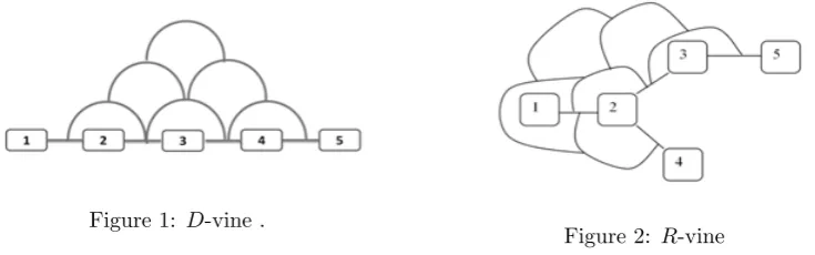
TheThumb Rulesays that if a density is represented on two regular vines whose top nodes

share a common element, then the product of all (conditional) copula containing that element

on one regular vine is equal to the product of all (conditional) copula containing that same

element in the other vine.

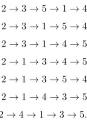
The thumb rule is illustrated with aD-vine with first tree 1-2-3-4-5 andR-vine in Figures

Figure 1: D-vine .

Figure 2: R-vine

If the same density is represented with (conditional) copulas on these two vines then the

marginal densities on nodes (1,. . . ,4) must be equal, and therefore, by the Thumb Rule the

product of all copula containing 5 must also be equal.

c4,5c3,5;4c2,5;4,3c5,1;4,3,2=c3,5c2,5;3c1,5;2,3c4,5;1,2,3.

The density for theR-vine above may be written:

f12345(x1, x2, x3, x4, x5) = f1(x1)f2(x2)f3(x3)f4(x4)f5(x5)c4,2c2,1c2,3

c3,5c4,1;2c1,3;2c2,5;3c4,3;1,2c1,5;2,3c4,5;1,2,3

= f5(x5)c3,5c2,5;3c1,5;2,3c4,5;1,2,3f4(x4)

c2,4c1,4;2c3,4;1,2f3(x3)c2,3c1,3;2f2(x2)c2,1f1(x1)

where the last expression simply re-arranges terms in the previous expression. Since

f12345(x1, x2, x3, x4, x5)

f1234(x1, x2, x3, x4)

=f5_|1234(x5|x1, x2, x3, x4)

we have

f5_|1234(x5|x1, x2, x3, x4) = f5(x5)c3,5c2,5;3c1,5;2,3c4,5;1,2,3,

f4|123(x4|x1, x2, x3) = f4(x4)c2,4c1,4;2c3,4;1,2,

f3|12(x3|x1, x2) = f3(x3)c2,3c1,3;2,

f2_|1(x2|x1) = f2(x2)c2,1.

This corresponds [4] to the familiar decomposition

f12345(x1, x2, x3, x4, x5) =f5|1234(x5|x1, x2, x3, x4)f4|123(x4|x1, x2, x3)f3|12(x3|x1, x2)f2|1(x2|x1)f1(x1).

Note that these conditional densities can be expressed as products of copula densities on the

R-vine and one dimensional margins of the regular vine decomposition and they correspond to

a sampling orderx1 →x2 →x3 →x4 →x5 in which each variable is sampled conditional on

its predecessors in the ordering.

Definition 3.1 (Sampling order implied by a regular vine). A sampling order for nvariables

for other variables are conditioned on the preceding variables in the ordering. A sampling order

is implied by an R-vine representation of the density if each conditional density can be written

as a product of copula densities in the vine and one dimensional margins.

Not all sampling orders are implied by anR-vine representation of the density. Following

sections show which sampling orders are implied by a givenR-vine representation. First, the

edging up algorithm is presented which samples an R-vine starting with an arbitrary variable.

4

Edging Up Sampling Algorithm

This section describes an algorithm for sampling a regular vine starting at an arbitrary element.

It does not require the constant conditional copula assumption. This is also an algorithm for

conditionalizing on a set of variables which is an initial segment of a sampling order. An

illustration is better than an abstract description; we illustrate with the R-vine in Figure 2.

The first two steps are shown in Figures 3 and 4. The edges are labeled in Figure 3 and omitted

in subsequent steps of the algorithm. We start with five independent samples of a [0,1] uniform

variableu1, u2, . . . , u5.

1. Pick a variable, say 2 and sample it as:

x2=F2−1(u2).

Figure 3: Edging up step 1

Figure 4: Edging up step 2

2. Pick an edge abutting the previously chosen element (see step 2 in Figure 4). A single

element in the constraint set of the last chosen edge is un-sampled, sample it as:

x3=F3−1C−

By proposition 2.1 this samples (X3|x2). x3 = F3−1C− 1

3_|2(u3) is shorthand for x3 =

F₃−1C₃−_|x1

2(u3). Similar shorthand notation is used below.

3. Pick an edge abutting the previously chosen element, the choice is shown in Figure 5:

Figure 5: Edging up step 3 Figure 6: Edging up step 4

A single element in the constraint set of the last chosen edge is un-sampled, sample it as:

x5=F5−1C−

1 5|3C−

1 5|32(u5).

By proposition 2.1 this samples (X5|x3, x2).

4. Pick an edge abutting the previously chosen element. A single element in the constraint

set of the last chosen edge is un-sampled, sample it as:

x1=F1−1C−

1 1|2C−

1 1|32C−

1 1|532(u1).

By proposition 2.1 this samples (X1|x5, x3, x2).

5. Pick an edge abutting the previously chosen element. A single element in the constraint

set of the last chosen edge is un-sampled, sample it as:

x4=F4−1C−

1 4|2C−

1 4|12C−

1 4|312C−

1 4|5312(u4).

By proposition 2.1 this samples (X4|x1, x2, x3, x5).

For theR-vine in Figure 2 there are seven possible sampling orders starting with 2:

2→3→5→1→4

2→3→1→5→4

2→3→1→4→5

2→1→3→4→5

2→1→3→5→4

2→1→4→3→5

An algorithm for generating implied sampling orders is presented in the next section.

5

Sampling Order and Merging Theorems

This section establishes a general result on the number of implied sampling orders for a regular

vine. This is important when we need to conditionalize the distribution represented as a regular

vine on observations. Conditionalizing such a distribution is very easy when the conditioning

variables appear as an initial segment of a sampling order for this vine. To sample the

condi-tional distribution it is enough to plug the values of the conditioning variables into the sampling

algorithm. If there is no sampling order for this vine that keeps all conditioning variables as an

initial segment one would need to transform the vine to another one. Such transformations are

in general cumbersome.

Theorem 5.1. Any regular vine on n variables implies2n−1_{sampling orders.}

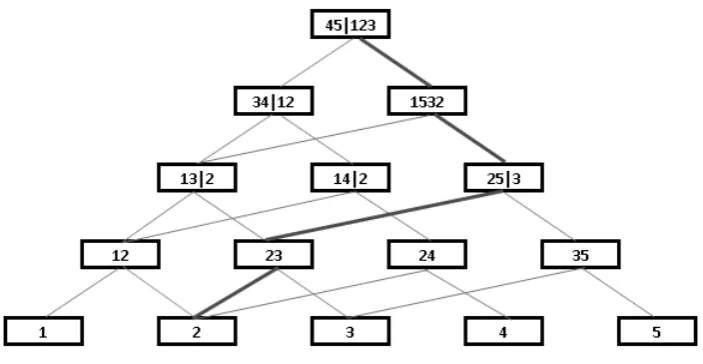
Proof: The proof proceeds by establishing a bijection between implied sampling orders and

increasing paths in a triangular array (an example is given in Figure 7). The array consists of

nechelons. At the bottom are the individual variables. Fori= 2, . . . , n, echelonicorresponds

to tree i−1 in theR-vine, and shows the conditioned and conditioning sets of the copulas on

tree i−1, i= 2, . . . , n. Draw lines representing the membership relations. Each application

of the edging up algorithm corresponds to a unique increasing path in the triangular array:

at each echelon there is one and only one variable in the conditioned set which is not present

in a conditioned set lower on the path. The proof is concluded by counting the number of

increasing paths in such a triangular array. Because each node in echelon i is an edge in tree

i−1;i = 2, . . . , n, the number of upward edges leaving a node is the degree of the node in

the vine, whereas the number of edges entering the bottom of each node above the first row

is always two. All paths terminate in the top node (echelon n) through one of the two edges

entering the top node. Each such path enters echelonn−1 through one of two paths. Counting

from the top node down, at echelonithe number of paths increases by a factor 2, i=n, . . . ,2.

Hence the number of increasing paths is 2n−1_.

With this proof in hand, it is easy to see that the following is a procedure for generating all

sampling orders. The algorithm is as follows

• Choose one variable from the top node’s conditioned variables, call itan.

• Truncate the vine by integratingan out. That is, remove all nodes containingan.

• The remaining sub-vine has two conditioned variables in its top node. Pick one call it

an₋1, and integrate it out etc.

The sequence of variables removed in this way in reverse order (a1, . . . , an) is a sampling order.

The triangular array for the R-vine in Figure 2 and the implied sampling order used to

illustrate the edging up algorithm are shown in Figure 7.

Figure 7: Triangular array forR-vine with sample order

It is easy to count the number of sampling orders emanating from each variable. In Figure

7 instead of writing the variables in each cell of the triangular array, write ‘1’ in the top cell. In

each other cell, write the sum of the numbers immediately above that cell. The results for the

D-vine andR-vine in Figures 1 and 2 are shown in Figures 8 and 9 where the variables’ indices

are written below the cells n in the first row. A simple function counts the implied sampling

orders starting with variablex. Ift is the top cell, puth(t) = 1 and for celli,

h(i) = ∑

j directly abovei

h(j), (5.1)

whereh(x) is the number of sampling orders starting with variablex.

Figure 8: Numbers of implied sample orders

for D-vine of Figure 1

Figure 9: Numbers of implied sample orders

We address a problem of merging two vines that are not overlapping into one larger vine.

Merging may be useful if we need to combine vine models of distinct subsets of random variables.

The number of possible such mergers is found. This result provides at once a shorter, more

intuitive and more general result of the theorem in [6] stating the number of regular vines.

Definition 5.1(Merger). A regular vineV(n+m)withn+mvariables is amergerof regular

vines A(n) on n variables and B(m) on m variables distinct from those in A(n) if A(n) and

B(m) are sub-vines ofV(n+m).

Theorem 5.2. For regular vinesA(n)on nvariables and B(m) onm variables distinct from

those inA(n), there are2n+m−2 _mergers.

Proof: LetA(n) have top conditioned variablesan,an−1, and B(m) have top conditioned

variables bm, bm−1. Suppose they are merged. The conditioned variables of the merged top

node are one ofan, an−1and one ofbm, bm−1. Suppose they arean, bm. Sincean is conditioned

with every other ai, in A(n), which goes from echelon 1 to n, an must be conditioned with

variables from vineB(m) in echelonsn+ 1, . . . , n+m.

Integrate out variablebm. The top node in vineB(m) is removed leaving aB(m−1)-subvine

with a new top node. The top node of the new merged subvine has a variable fromB(m−1) in

its conditioned set, and this variable must occur in the new top node of theB(m−1)-subvine.

Call this variablebm−1. In the new merged subvinebm−1 is partnered withan. Now integrate

bm−1out of the merged subvine. A new variable, call itbm−2, appears conditioned withan and

bm−2in the resulting merged subvine.

Proceeding in this way, the sequence (bm, bm₋1, . . . , b1) occurs as top conditioned variables

in successive subvines of B(m), and also as partners of an in decreasing echelons. It is a

reverse sampling order for B(m). By parity of reasoning, the same holds for the sequence

(an, an−1, . . . , a1) which is a reverse sampling order ofA(n).

Going back to the merged subvine after integrating out bm, its top node’s conditioned

variables arean, bm₋1. Now integrate out successively theai’s. By the above argument applied

to this subvine, the sequence of partners ofbm−1 obtained is a reverse sampling order. Denote

this sampling order (an, ax, . . . , ay). We claim that (an, ax, . . . ay) = (an, an−1, . . . , a1). Indeed,

the node with conditioned variablesax, bm−1 must be a child ofbm, an−1from which it follows

that ax=an₋1, and similarly forbm₋2, bm₋3, . . . , b1.

We have shown, for any i, that the partners of ai are a reverse sampling order starting

with the reverse sampling order (bm, bm−1, . . . , b1) followed by the reverse sampling order of

A(n) after integrating outan, . . . , ai+1. Mutatis mutandis forB(m). This shows that a merger

of A(n) andB(m) defines a unique sampling order of each ofA(n) andB(m). Also, given a

sampling order of A(n) and of B(m), it is easy to verify that we can construct a merger by

choosing partners ofaiandbj from the sampling order ofB(m) andA(n) respectively; whereby

the conditioning variables are the variables ofB(m) andA(n) which must be integrated out to

Form= 1, this result says that there are 2n−1_{extensions of a regular vine onn variables.}

[6] showed that for a naturally ordered regular vine on n elements, there are 2n−2 naturally

ordered regular vines onn+ 1 elements which extend this regular vine. As there are two natural

orderings, these two results agree. The present proof is much shorter. The number of naturally

ordered regular vines on n variables is 2(

n−2 2 )

, the number of regular vines on n variables is

(n

2

)

(n−2)!2( n−2

2 )

.

In the Table 1 eight possible mergers of twoD-vines 2−1−3 and 4−5 are given. We

present conditioned and conditioning sets of nodes in the mergers that do not belong to the

D-vines.

NR echelon 5 echelon 4 echelon 3 echelon 2

1 24|135 25|13, 34|15 35|1, 14|5 15

2 24|135 25|13, 14|35 15|3, 34|5 35

3 25|134 24|13, 35|14 34|1, 15|4 14

4 25|134 24|13, 15|34 14|3, 35|4 34

5 34|125 35|12, 14|25 15|2, 24|5 25

6 34|125 35|12, 24|15 25|1, 14|5 15

7 35|124 34|12, 15|24 14|2, 25|4 24

8 35|124 34|12, 25|14 24|1, 15|4 14

Table 1: Conditioning and conditioned sets of the mergers that do not belong toD-vines 2−1−3

and 4−5.

6

Plug in Conditionalization and Sample Order Proximity

We can conditionalize on any initial segment of any sampling order by simply plugging in values.

Referring to the R-vine in Section 4, we could plug x2, x3 and x1 into the edging up example

and conditionalize on these three values. Suppose we want to conditionalize on variables 2 and

5; none of the sampling orders implied by this R-vine have {2,5} as an initial segment. To

enable plug in conditionalizing we must transform the R-vine in such a way that variables 2

and 5 are contiguous. Consider theR-vine obtained by switching positions of variables 2 and

3. The sampling order 2→5→3→1→4 becomes available. The conditional densities are

f2, f5|2, f3|5,2, f1|3,5,2, f4|1,3,5,2.

Note thatf1|3,5,2, f4|1,3,5,2are already available as products of copula densities from the original

R-vine; they don’t need to be re-computed. To computef5_|2, f3_|5,2 we apply the Thumb Rule

to 2,3,5:

The terms on the left hand side are available from the original R-vine. We need to compute

c2,5 and then solve forc5,3;2. From c2,5 we obtainf5_|2andf3_|5,2=c5,3;2c2,3f3.

In searching for ‘neighboring’R-vines to enable plug in conditionalization, or in searching

the space ofR-vines efficiently, it may be useful to have a notion of proximity.

Definition 6.1(Sample order proximity). The sample order proximity of twoR-vinesA(n),B(n)

on nvariables is the number of common sampling orders implied byA(n) andB(n).

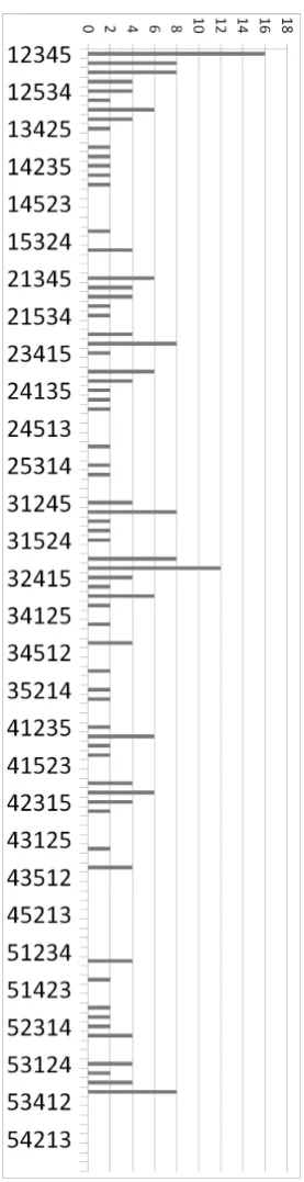
Figure 10 shows for each of the 120 permutations of the 5 variables in theR-vine in section 4,

the number of common sampling orders with the originalR-vine. The permutations are shown

as the result of permuting the lexigraphical order; thus (1,2,3,4,5) is the identity permutation,

(1,2,3,5,4) is the permutation switching 5 and 4, etc.

For each permutation in Figure 10, the number of implied sampling orders is 2n−1 _{= 16.}

The top permutation (1,2,3,4,5) corresponding to the originalR-vine has 16 common sample

orders, other permutations have fewer. The total number of common sampling orders shown in

Figure 10 is 22(n−1)= 28= 256, and this seems to hold for any regular vine and anyn, though

a proof is not available at this point. There are 52 permutations of theR-vine which have no

common sampling orders with the initialR-vine. The following proposition gives a lower bound

on the number of permutations with zero common sampling orders with a givenR-vine, which

does not depend on theR-vine being permuted.

Proposition 6.1. Let(a1, . . . , an),(b1, . . . , bn)be permutations of(1, . . . , n). LetA(a1, . . . , an)

be an R-vine on n variables where the variables are ordered according to the highest echelon

in which they appear as conditioned variables: {a1, a2} are conditioned variables in the top

node (echelon n), a3 and (possibly) a4 are conditioned variables in echelon (n−1), etc. Let

B(b1, . . . , bn) be another R-vine on n variables, similarly ordered. Then the number of

per-mutations π ∈ n! for which B(π−1_(b

1), . . . , π−1(bn)) has no common sampling orders with

A(a1, . . . , an)is greater or equal to (n−2)(n−3)(n−2)! + 4(n−3)2.

Proof: There can be no common sampling orders for permutations under which the

con-ditioned variables in the top node of B do not occur in the top node of A(a1, . . . , an). This

number is

#{π∈n!|π−1(b1)∈ {/ a1, a2}, π−1(b2)∈ {/ a1, a2}}= (n−2)(n−3)(n−2)!

If a permutation preserves one of the top conditioned variables, say x, but has no common

element in echelon (n−1) for the node not containingx, then there can be no common sample

orders. Ifa3, a4 are both in echelonn−1 then this number is

#{π∈n!|π−1(b1)∈ {a1, a2}, π−1(b2)∈ {/ a1, a2, a4}, π−1(b4)∈ {/ a1, a2, a4}} ≥2(n−3)(n−3)

(6.1)

Ifa4is not in echelonn−1, thena3replacesa4 in Equation 6.1, without affecting the number

of permutations.

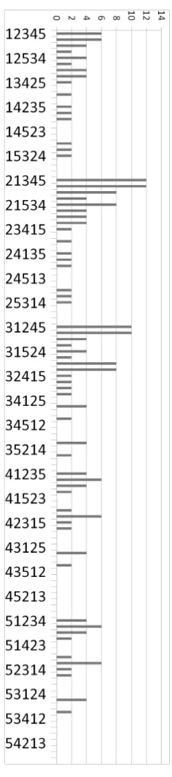
In the casen= 5, the above estimate is exact, and the number of permutations ofBhaving

no common sampling orders withAis 36 + 8 + 8 = 52. Figure 11 shows the number of common

sampling orders with the originalR-vine, for all permutations of aCvine onnvariables. The

distribution of numbers of common sampling orders is different from that in Figure 10, though

the total numbers are the same as is the number of permutations with zero common sample

orders.

The space of regular R-vines is very large. In searching for a vine which optimally fits

a multivariate data set, heuristics are employed to restrict the search space. The sampling

order proximity may provide a useful heuristic, as we may wish to restrict the initial search to

vines which have a low number of common sampling orders in common. If we are searching

to optimize some scalar function of R-vines and if this function is related to the vine structure

as captured in sampling orders, then a low proximity search heuristic may yield good starting

points for searches in a small number of neighborhoods.

7

Illustrative Example

We consider the financial data first analysed using vines in [13]. The data represent four time

series of daily data: (1) the SSBWG hedged bond index, (2) the MSCI world stock index, (3)

the Norwegian stock index (TOTX) and (4) the Norwegian bond index (BRIX), for the period

from 04.01.1999 to 08.07.2003. Prior to fitting a vine to these data, the conditional mean is

modelled using a first order autoregression and the conditional variance is modelled using a

GARCH(1, 1) process. The remaining analysis is then run on the residuals. These initial steps

follow exactly those given in [13].

The Kendall rank correlations between each of the variables are given in Table 2. We see that

there are both positive and negative associations in the data, with the strongest being between

the MSCI and TOTX indexes and SSBWG and BRIX indexes. Both of these relationships are

positive.

SSBWG(1) MSCI(2) TOTX(3) BRIX(4)

SSBWG(1) 1.00 -0.16 -0.13 0.22

MSCI(2) -0.16 1.00 0.33 -0.04

TOTX(3) -0.13 0.33 1.00 -0.11

BRIX(4) 0.22 -0.04 -0.11 1.00

Table 2: The Kendall rank correlations between the 4 variables.

Initially we fit a D-vine to the 4 time series using the VineCopula [?] and CDVine [?]

packages in R [5]. To do so we specify a structure and then bivariate copulas are selected from

highest AIC value. The parameters of these copulas are estimated using maximum likelihood.

The initial structure chosen is arbitrary in order to allow us to consider changes to the structure

to improve the fit using the methods in the paper.

The chosen vine structure, bivariate copulas and fitted Kendall correlation values are given

in Figure 12.

We see the structure of the vine. In the first tree the copula with the highest AIC between

SSBWG and TOTX is the Normal copula, between TOTX and BRIX is the rotated 90 degrees

Gumbel copula and between BRIX and MSCI is the Frank-copula. The t-copula is chosen

between all variables in the second and third trees.

We can use the edging up algorithm to sample from the vine. To do so we use the method in

Section 4. Suppose we wish to sample from the vine in the order (BRIX,TOTX,SSBWG,MSCI)=

(4,3,1,2). Suppose we have sampled 4 uniform random variables (u1, u2, u3, u4). We can then

use the edging up algorithm to sample;

x4 = F4−1(u4),

x3 = F3−1

(

C₃−_|41(u3)

)

,

x1 = F1−1

(

C₁−_|31

(

C₁−_|1₃₄(u1)

))

,

x2 = F2−1

(

C₂−_|41

(

C₂−_|1₃₄

(

C₂−_|1341 (u2)

)))

.

We take 1000 samples. To show that the edging up algorithm is retaining the vine structure

we need to check that the marginal distributions of the four variables are still uniform and the

Kendall correlations are being preserved. We give histograms of the four variables in Figure

13.

We see that all four of the samples from the marginal distributions of the variables show

uniform distributions on [0,1]. Thus, marginally, the edging up algorithm is doing a good job.

We consider the dependence between the different variables in the sample. Bivariate scatter

plots between each pair of variables are given in Figure 14.

From the scatterplots we see the positive correlations between MSCI and TOTX and

SS-BWG and BRIX as remarked on the correlations table from the data (Table 2) and we also see

negative correlations between SSBWG and TOTX and BRIX and TOTX.

The correlation between the simulated values for MSCI and TOTX is 0.35, between SSBWG

and BRIX is 0.21 and between SSBWG and TOTX is -0.14. These values all show good

agreement with the values from the data.

We consider the optimal selection of a vine structure for these data. The log-likelihood for

the vine considered is 278.31 and the AIC is -538.63. A search of all of the possible D-vine

structures, and performing the sequential estimation of the copulas within each vine using the

VineCopula package, results in the optimal vine measured using both log-likelihood and AIC

t-, rotated Joe and rotated Gumbel. The log-likelihood of this optimal vine and the AIC are

292.56 and -567.13 respectively.

Let us return to the vine in Figure 12. There are 24−1= 8 possible sampling orders for this vine. They are:

2 → 4 → 3 → 1

4 → 2 → 3 → 1

4 → 3 → 2 → 1

4 → 3 → 1 → 2

3 → 4 → 2 → 1

3 → 2 → 4 → 1

3 → 2 → 1 → 4

4 → 3 → 2 → 1

We wish to improve the fit of our vine. To do so we consider the permutations of the vine

with a low number of sampling orders in common with this vine. There are two D-vines with

0 common sampling orders with this vine. The first tree of each of these vines, using the first

letter as shorthand for each variable, along with the log-likelihood and AIC of each vine, are

given in Table 3. The log-likelihood and AIC of the original vine and optimal vine are given

below for comparison.

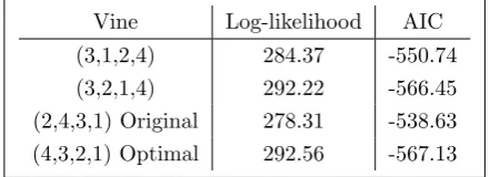
Vine Log-likelihood AIC

(3,1,2,4) 284.37 -550.74

(3,2,1,4) 292.22 -566.45

(2,4,3,1) Original 278.31 -538.63

(4,3,2,1) Optimal 292.56 -567.13

Table 3: The log-likelihood and AIC of each of theD-vines with no common sampling orders

to the original vine.

We see that both of the vines with 0 sampling orders in common with the original vine have

better fit, in terms of both log-likelihood and AIC, than the original vine. The second of these

vines, with first tree (3,2,1,4), has a log-likelihood and AIC which are very close to those of

the optimal vine: just 0.34 and 0.68 lower respectively. Thus by considering permutations with

low proxoimity to the original vine we have found a vine which is very close to optimal. The

optimal vine has just 2 sampling orders in common with the original vine.

The conjecture is that a ”low proximity search” would give an efficient coarse grained way

of searching the space of regular vines. This example is really too small to offer much support,

indeed there are only 12 distinctD−vines on 4 variables. Nonetheless, we compare two search

strategies, (1) choose 3 random permutations, compute theAICof each and pick the minimum,

and (2) pick one random permutation, compute itsAICand theAIC’s of the two permutations

with no common sampling order with the randomly chosen permutation, take the minimum.

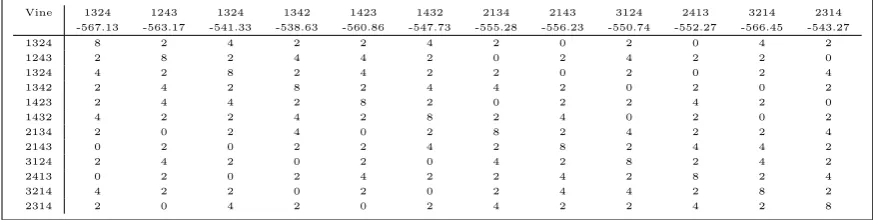
chance (62%) of reaching a lowerAIC. Table 4 gives a proximity matrix and theAIC values

for each permutation. Of course, the efficacy of this heuristic depends on the relation between

the scalar function we wish to optimize and the vine structure as captured in the proximity

relation. Using the loglikelihood instead of theAIC would give no advantage to the proximity

heuristic.

Vine 1324 1243 1324 1342 1423 1432 2134 2143 3124 2413 3214 2314 -567.13 -563.17 -541.33 -538.63 -560.86 -547.73 -555.28 -556.23 -550.74 -552.27 -566.45 -543.27

1324 8 2 4 2 2 4 2 0 2 0 4 2

1243 2 8 2 4 4 2 0 2 4 2 2 0

1324 4 2 8 2 4 2 2 0 2 0 2 4

1342 2 4 2 8 2 4 4 2 0 2 0 2

1423 2 4 4 2 8 2 0 2 2 4 2 0

1432 4 2 2 4 2 8 2 4 0 2 0 2

2134 2 0 2 4 0 2 8 2 4 2 2 4

2143 0 2 0 2 2 4 2 8 2 4 4 2

3124 2 4 2 0 2 0 4 2 8 2 4 2

2413 0 2 0 2 4 2 2 4 2 8 2 4

3214 4 2 2 0 2 0 2 4 4 2 8 2

2314 2 0 4 2 0 2 4 2 2 4 2 8

)

Table 4: The AIC of each of theD-vines with no common sampling orders to the original vine.

8

Conclusions

Regular vines are a powerful modeling tool for data analysis and uncertainty propagation. To

be used in “live decision support” regular vines must handle large data sets and must enable

rapid conditionalization. This paper shows that there are promising lines of attack on these

problems. Vine space grows very rapidly in the number of variables and the notion of sampling

proximity may enable searching this space efficiently by stepping over vines that are close in

this sense. Rapid conditionalization can be based on the edging up algorithm if the conditioned

variables form an initial segment of an implied sample order. When that is not the case, the

thumb rule may help limit the number of calculations required to place the conditioned variables

in an initial segment of an implied sampling order.

References

[1] Harry Joe. Multivariate extreme-value distributions with applications to environmental data.The

Canadian Journal of Statistics / La Revue Canadienne de Statistique, 22(1):pp. 47–64, 1994.

[2] R.M. Cooke. Markov and entropy properties of tree and vine-dependent variables. InProceedings of the ASA Section on Bayesian Statistical Science,, 1997.

[3] Cooke R.M., Joe H., and Aas K. Vines arise. InDependence Modeling: Handbook on Vine Copulae,

2010.

[4] Aas K.and Czado C.and Frigessi A. and Bakken H. Pair-copula constructions of multiple depen-dence. Insurance: Mathematics and Economics, 44(2):182–198, 2009.

[6] Oswaldo Moralees Napoles. PhDF Thesis Bayesian Belief Nets and Vines in Aviation Safety and

Other Applications. Department of Mathematics, Delft University of Technology, Delft, 2009.

[7] T.J. Bedford and R.M. Cooke. Probability density decomposition for conditionally dependent random variables modelled by vines.Annals of Mathematics and Artificial Intelligence, 32(4):245–

268, 2001.

[8] Bedford T.J. and Cooke R.M. Vines - a new graphical model for dependent random variables.

Ann. Statist, 30:1031–1068, 2002.

[9] Harry Joe. Dependence Modeling with Copulas. Chapman & Hall, CRC., 2014.

[10] Jakob Stoeber, Harry Joe, and Claudia Czado. Simplified pair copula constructions, limitations

and extensions. Journal of Multivariate Analysis, 119:101 – 118, 2013.

[11] I. Hobaek Haff, K. Aas, and A. Frigessi. On the simplified pair-copula construction - simply useful or too simplistic? Journal of Multivariate Analysis, 101:1296–1310, 2010.

[12] D. Kurowicka and R.M. Cooke. Uncertainty Analysis with High Dimensional Dependence Mod-elling. Wiley, 2006.

[13] K. Aas, K. C. Czado, A. Frigessi, and H. Bakken. Pair-copula constructions of multiple dependence.

9

Appendix: Regular Vines

Definition 9.1 (Regular vine). V is a regular vine onnelements if

1. V={T1, . . . , Tn₋1},

2. T1 is a connected tree with nodes N1={1, . . . , n}, and edgesE1;

fori= 2, . . . , n−1 Ti is a tree with nodes Ni=Ei−1.

3. (proximity)fori= 2, . . . , n−1, {a, b} ∈Ei,|a△b|= 2 where△ denotes the symmetric

difference and|A| denotes the number of elements in setA.

A D-vineis a regular vine in which each node in each tree has degree at most 2; a C-vine is

a regular vine in which each tree has one node of maximal degree, other nodes having degree 1.

Definition 9.2 (constraint, conditioning, conditioned sets).

1. For e∈Ei, i≤n−1, the constraint setassociated with eis the complete union Ue∗

ofe, that is, the subset of {1, . . . , n} reachable from eby the membership relation.

2. Fori= 1, . . . , n−1, e∈Ei, ife={j, k}then the conditioning setassociated witheis

De=Uj∗∩Uk∗

and theconditioned set associated withe is

{Ce,j, Ce,k}={Uj∗\De, Uk∗\De}.

3. The order of an edgee∈Ej is the cardinality of its conditioning set, and isj−1.

4. A node belongs toechelonξifξis the cardinality of its constraint set. Individual variables

belong to the first echelon.

Note that a node in treek is an edge in treek−1,k >1; therefore referencing a node by

its tree can be ambiguous. The echelon designation removes this ambiguity. With nvariables,

there arenechelons, the top echelon (echelonn) contains one element, namely the unique node

in echelonnthat is an unique edge in tree n−1. Note that fore∈E1, the conditioning set is

empty and its order is 0. Fore∈Ei, i≤n−1, e={j, k}we have Ue∗=Uj∗∪Uk∗.

Definition 9.3 (child, descendent). If node e is an element of node f, we say that e is an

childof f; similarly, if eis reachable from f via the membership relation: e∈e1∈...∈f, we

say thateis an descendent off.

Lemma 9.1. [12] For any nodeM of orderk >0 in a regular vine, if elementi is a member

of the conditioned set of M, then i is a member of the conditioned set of exactly one of the

children of M, and the conditioning set of an child ofM is a subset of the conditioning set of

Definition 9.4(parents, siblings). If elementaoccurs with elementb as conditioned variables

in echelon k > 1, then a andb are termed k-partners. NodesA andB are siblings if they

are children of a common parent. A consanguineous grandchildof node e∈Ei, i > 1 is a

node which is a child of two children of e.

Definition 9.5(natural order). Anatural orderof the elements of a regular vineV(n)onn

elements is a sequence of numbers N O(V(n)) = (An, An−1, ..., A1)where each Ai is an integer

not greater thannobtained as follows: Take one conditioned element of echelon nof a regular

vine and assign it position n; assign itsn-partner position (n−1). Element An₋1 occurs with

an(n−1)-partner in the conditioned set of one child of the top node. Give this(n−1)-partner

position(n−2). The(n−2) partner of elementAn−2 is assigned position(n−3). Iterate this

process until all elements have been assigned a position. Position1is assigned to the2−partner

of the variable in position 2.

Figure 11: Number of common sampling orders with the R-vine for each permutation of a

Figure 12: TheD-vine fitted to the Norwegian stock market data.

SSBWG

Frequency

0.0 0.2 0.4 0.6 0.8 1.0

0

20

40

60

80

100

TOTX

Frequency

0.0 0.2 0.4 0.6 0.8 1.0

0

20

40

60

80

100

BRIX

Frequency

0.0 0.2 0.4 0.6 0.8 1.0

0

20

40

60

80

100

MSCI

Frequency

0.0 0.2 0.4 0.6 0.8 1.0

0

20

40

60

80

100

Figure 13: Histograms of the samples from the four variables showing the preservation of the

Scatter Plot Matrix SSBWG

0.6 0.8 1.0

0.6 0.8 1.0

0.0 0.2 0.4

0.0 0.2 0.4

TOTX

0.6 0.8 1.0

0.6 0.8 1.0

0.0 0.2 0.4

0.0 0.2 0.4

BRIX

0.6 0.8 1.0

0.6 0.8 1.0

0.0 0.2 0.4

0.0 0.2 0.4

MSCI

0.6 0.8 1.0

0.6 0.8 1.0

0.0 0.2 0.4

0.0 0.2 0.4

Figure 14: Bivariate Scatter plots between each of the four variables showing the dependence