November 24, 2014
Benchmarking atomic Data for Astrophysics: Si
iii
⋆
G. Del Zanna
1, L. Fern´andez-Menchero
2, and N. R. Badnell
21 DAMTP, Centre for Mathematical Sciences, Wilberforce Road, Cambridge, CB3 0WA, UK 2 Department of Physics, University of Strathclyde, Glasgow, G4 0NG, UK
Received ; accepted
ABSTRACT
We investigate the main spectral diagnostics for SiiiiUV lines, which have been previously used to measure electron densities, temper-atures, and to suggest that non-Maxwellian electron distributions might be present in the low transition region of the solar atmosphere. Previous atomic calculations and observations are reviewed. We benchmark the observations using a new large-scale R-matrix scat-tering calculation for electron collisional excitation of Siiii, carried out with the intermediate-coupling frame transformation method (ICFT). We find generally good agreement between predicted and observed line intensities, if one takes into account the different temperature sensitivity of the lines, and the structure of the solar transition region. We find no conclusive evidence for the presence of non-Maxwellian electron distributions.
Key words.Atomic data – Line: identification – Sun: corona – Techniques: spectroscopic
1. Introduction
Siiiilines are prominent in UV spectra of solar and many
as-trophysical plasmas (planetary nebulae, novae, stars, interstellar medium). They have been used for a variety of diagnostic ap-plications, in particular to measure electron densities and tem-peratures. For example, Dufton et al. (1983) used Skylab ob-servations obtained with the Naval Research Laboratory (NRL) slit spectrograph S082B to measure electron densities. Some discrepancies between observed and predicted line ratios were found. They involved the intercombination line 3s2 1S
0– 3s 3p 3P
1at 1892 Å and the 3s 3p1P1–3s 4s1S01312.6 Å line. Dufton et al. (1984) suggested that these discrepancies could have been caused by the presence of non-Maxwellian electron distributions in the low transition region. The upper level of the 1312.6 Å line is populated from the ground state via a transition with a relatively high excitation energy, hence would be sensitive to the high-energy tail of any non-Maxwellian electron distribu-tion. Since then, various authors have used solar observations of Siiiilines to suggest that non-Maxwellian electron distributions
were present in the solar corona (see, e.g. Keenan et al. 1989; Pinfield et al. 1999; Dzifˇc´akov´a & Kulinov´a 2011).
Clearly, it would be extremely interesting if non-Maxwellian electrons were present in the solar transition region. However, it is important beforehand to analyse the atomic data for this ion. This is done here by carrying out new atomic calculations and then reassessing the diagnostics using various solar and stel-lar observations. The scattering calculations are part of our UK APAP network work along the Mg-like sequence (Fern´andez-Menchero et al. 2014).
We first briefly review in Sect. 2 previous calculations for this ion. Sect. 3 presents our calculations, while Sect. 4 presents our comparisons with observations. We present in Sect. 5 our conclusions.
⋆ The full dataset (energies, transition probabilities and rates)
are available in electronic form at our APAP website (www.apap-network.org)
2. Previous calculations
2.1. Scattering calculations
Baluja & Hibbert (1980) used the CIV3 program (Hibbert 1975) to calculate wavefunctions and energies for the lowest 12 LS terms, which give rise to 20 fine-structure levels. The complete set of n=3,4 configurations was adopted. These wavefunctions were later used for the scattering calculations for this ion with
R-matrix codes in a series of papers (Baluja et al. 1980, 1981;
Dufton et al. 1984). A paper that has been widely cited was that of Dufton & Kingston (1989), because the level-resolved effective collision strengths were made available in a tabulated form. These data were made available in the first version of the CHIANTI database (Dere et al. 1997) and are still in the last one, v.7.1 (Landi et al. 2013). Dufton & Kingston (1989) performed the calculations in LS coupling, including partial waves up to
L=12, for about 1050 impact energies (up to 10 Ryd). They then used the JAJOM code (Saraph 1978) to obtain level-resolved collision strengths.
Griffin et al. (1999) performed an ICFT R-matrix calcula-tion, with an LS close-coupling expansion which included all 25 terms arising from the 3s2, 3s 3p, 3p2, 3s 3d, 3p 3d, 3d2, 3s 4s, 3s 4p, and 3s 4d configurations. A full exchange calculation was performed on all partial waves up to L=12, using 25 contin-uum basis orbitals. A non-exchange calculation in LS coupling for L=10–50 was performed, and added, together with the usual top-up for high J contributions, to the exchange part. The num-ber of mesh points used in the asymptotic part of the problem was 5032 and the maximum energy was 7.35 Ryd.
2.2. Transition probabilities
That radiative rates for several Siiiitransitions differed
signifi-cantly from one another was well known in the literature. Griffin et al. (1999) also suggested that several of the diagnostic line ra-tios commonly used could be significantly different, depending on which radiative rates one employs.
2.2.1. The intercombination line
The transition probability for the intercombination line 3s2 1S 0– 3s 3p3P
1at 1892.0 Å has been the subject of many studies, be-cause its value varies significantly between calculations. The3P1 level has a weak mixing with the1P
1level through the spin-orbit parameter of the 3p electron, so the radiative rate is sensitive to the energies of these levels. It turns out that ab-initio calcula-tions are unable to obtain the energy of the 3s 3p3P
Jlevels close enough to the experimental value, so many authors have applied empirical corrections.
Baluja & Hibbert (1980) provided a radiative rate of 1.2×10⁴ s−1. Dufton et al. (1983) improved the Baluja & Hibbert (1980) calculations, by adjusting the diagonal energies of the Hamiltonian matrix (to reproduce the experimental energies), to obtain a value of 1.46×10⁴s−1, which has been widely used since.
Nussbaumer (1986) used the superstructure program
(Eissner et al. 1974) and different basis sets (66 and 120 config-urations up to n=8) to try to improve the energies of the lowest levels. At the end, the term energies were still not very accurate, so various semi-empirical corrections based on the observed en-ergies were applied to the calculations. Nussbaumer (1986) ob-tained a value of 1.8×10⁴ s−1. The atomic structure employed by Griffin et al. (1999) for the scattering calculation provided a lower value of 0.92×10⁴s−1. The energy-adjusted MCHF calcu-lations of Tachiev and Froese Fisher (2002)1 produced a value of 1.75×10⁴s−1.
There is only one experiment, by Kwong et al. (1983), which produced lifetime measurements and an A-value of 1.67±0.1×10⁴s−1. Various authors have adopted this experimen-tal value for modelling. We also adopt it here, as discussed be-low, although we note that further measurements would be use-ful, to confirm this value.
We also note that Ojha et al. (1988) obtained the same value measured by Kwong et al. (1983). Laughlin & Victor (1979) car-ried out semi-empirical model potential calculations for the in-tercombination line along the Mg-like sequence. They also ob-tained a value close to experiment, 1.78×10⁴s−1.
2.2.2. The 1312.6 Å line
Despite its diagnostic importance in terms of non-Maxwellian electron distributions, the calculation of the radiative rate for the 3s 3p 1P
1–3s 4s 1S0 1312.6 Å transition has received less at-tention from previous authors. Baluja & Hibbert (1980) noted that the inclusion of a 5s pseudo-orbital decreased the oscil-lator strength for this transition by a large factor, of three. In their model ion, Dufton et al. (1983) adopted the lower value calculated by Baluja & Hibbert (1980), which implies a tran-sition rate of 2.84×10⁸ s−1. The ab-initio value obtained by Griffin et al. (1999) is even lower, 1.81×10⁸ s−1. Nussbaumer (1986) provided instead a much larger value of 4.0×10⁸ s−1.
1 See http://nlte.nist.gov/MCHF/
The energy-adjusted MCHF calculations of Tachiev and Froese Fisher (2002) produced an even larger value, 8.87×10⁸s−1.
3. Atomic calculations
Several authors in the previous literature pointed out the signif-icant increases in the collision strengths calculated with the R-matrix codes, with respect to earlier distorted wave calculations. These are due to the resonances (see, e.g. Seaton 1975; Burke & Robb 1975). Our recent work on the more complex iron coronal ions (see. e.g. Del Zanna et al. 2012) has shown that larger tar-gets often produce significant increases in the level populations, partly because of enhanced resonances, partly because of cas-cading from higher levels. We have therefore set out to perform a larger scattering calculation to see what effects additional lev-els have. Our target, described below, includes the 3s 4f levlev-els, which in principle produce lines observed in the solar spectrum, and all the main n=5 levels, to improve the calculations for the
n=4 levels.
[image:2.595.310.464.348.523.2]3.1. The atomic structure
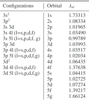
Table 1. The target electron configuration basis and orbital scaling
pa-rametersλnl.
Configurations Orbital λnl
3s2 1s 1.73313
3p2 2s 1.08334
3s 3d 2p 1.01965
3s 4l (l=s,p,d,f) 3s 1.03490 3s 5l (l=s,p,d,f, g) 3p 0.99789
3p 3d 3d 1.03993
3p 4l (l=s,p,d,f) 4s 1.03517 3p 5l (l=s,p,d,f,g) 4p 1.02034
3d2 4d 1.06435
3d 4l (l=s,p,d,f) 4f 1.37638 3d 5l (l=s,p,d,f,g) 5s 1.04415 5p 1.02725 5d 1.07274 5f 1.39217 5g 1.66124
The atomic structure calculations were carried out using the
autostructureprogram (Badnell 2011) which constructs target
wavefunctions using radial wavefunctions calculated in a scaled Thomas-Fermi-Dirac-Amaldi statistical model potential with a set of scaling parameters, in the same way as the superstruc -tureprogram (Eissner et al. 1974). The program also provides
radiative rates and infinite energy Born limits, used in the inter-polation of the collision strengths at high energies.
We have chosen as our configuration basis the set of 33 n=
3,4,5 configurations listed in Table 1. They give rise to 149 LS terms and 283 fine-structure levels. The scaling parameters λnl for the potentials in which the orbital functions are calculated are also given in Table 1.
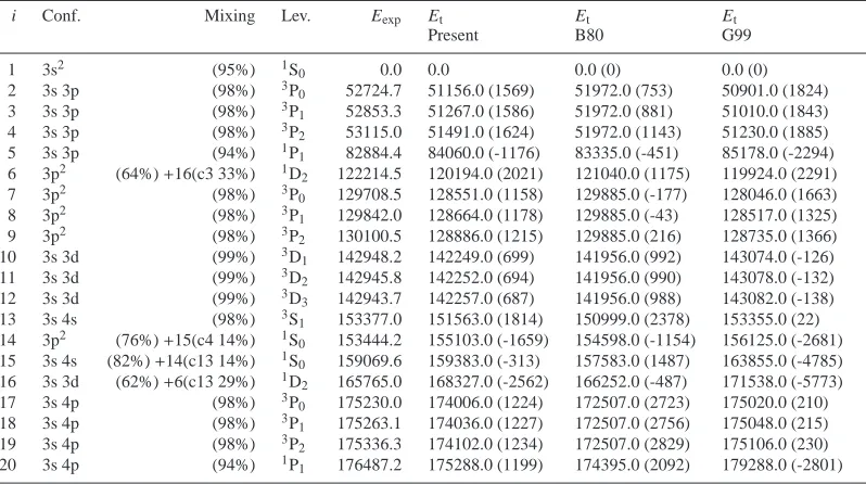
Table 2. Level energies for Siiii.
i Conf. Mixing Lev. Eexp Et Et Et
Present B80 G99
1 3s2 (95%) 1S
0 0.0 0.0 0.0 (0) 0.0 (0)
2 3s 3p (98%) 3P0 52724.7 51156.0 (1569) 51972.0 (753) 50901.0 (1824)
3 3s 3p (98%) 3P
1 52853.3 51267.0 (1586) 51972.0 (881) 51010.0 (1843)
4 3s 3p (98%) 3P
2 53115.0 51491.0 (1624) 51972.0 (1143) 51230.0 (1885)
5 3s 3p (94%) 1P1 82884.4 84060.0 (-1176) 83335.0 (-451) 85178.0 (-2294)
6 3p2 (64%)+16(c3 33%) 1D
2 122214.5 120194.0 (2021) 121040.0 (1175) 119924.0 (2291)
7 3p2 (98%) 3P
0 129708.5 128551.0 (1158) 129885.0 (-177) 128046.0 (1663)
8 3p2 (98%) 3P
1 129842.0 128664.0 (1178) 129885.0 (-43) 128517.0 (1325)
9 3p2 (98%) 3P
2 130100.5 128886.0 (1215) 129885.0 (216) 128735.0 (1366)
10 3s 3d (99%) 3D1 142948.2 142249.0 (699) 141956.0 (992) 143074.0 (-126)
11 3s 3d (99%) 3D
2 142945.8 142252.0 (694) 141956.0 (990) 143078.0 (-132)
12 3s 3d (99%) 3D
3 142943.7 142257.0 (687) 141956.0 (988) 143082.0 (-138)
13 3s 4s (98%) 3S1 153377.0 151563.0 (1814) 150999.0 (2378) 153355.0 (22)
14 3p2 (76%)+15(c4 14%) 1S
0 153444.2 155103.0 (-1659) 154598.0 (-1154) 156125.0 (-2681)
15 3s 4s (82%)+14(c13 14%) 1S
0 159069.6 159383.0 (-313) 157583.0 (1487) 163855.0 (-4785)
16 3s 3d (62%)+6(c13 29%) 1D
2 165765.0 168327.0 (-2562) 166252.0 (-487) 171538.0 (-5773)
17 3s 4p (98%) 3P
0 175230.0 174006.0 (1224) 172507.0 (2723) 175020.0 (210)
18 3s 4p (98%) 3P1 175263.1 174036.0 (1227) 172507.0 (2756) 175048.0 (215)
19 3s 4p (98%) 3P
2 175336.3 174102.0 (1234) 172507.0 (2829) 175106.0 (230)
20 3s 4p (94%) 1P
1 176487.2 175288.0 (1199) 174395.0 (2092) 179288.0 (-2801)
Notes. The experimental level energies Eexp(cm−1) are shown (see text), together with those obtained from our scattering target Et. Values in
parentheses indicate differences with Eexp. B80: Baluja & Hibbert (1980); G99: Griffin et al. (1999). Only the lowest 20 levels are shown.
(1999) values. Overall, we have very good agreement between observed and predicted energies, although as we mentioned the small discrepancy in the 3s 3p3P
Jlevels affects the radiative rate for the intercombination line.
We note that our target energies are worse than those of Baluja & Hibbert (1980), but better than those of Griffin et al. (1999) for all levels below the 3s 3d 3D
1 level. The diff er-ences in the various targets do not significantly affect the oscilla-tor strengths (and collisions strengths) for transitions involving these lowest 20 levels, with the exception of levels No. 14, 15. This occurs because the 3s 4s 1S0 level (No. 15) is LS -mixed with the nearby 3p2 1S
0level (No. 14). It turns out that the radia-tive rate for the 5–15 3s 3p1P
1–3s 4s1S01312.6 Å transition is very sensitive to the target wavefunctions. We have carried out several calculations, to try and establish an accurate value. The minimization procedure that we employed to obtain the scaling parameters shown in Table 1 resulted in an energy difference of 4280 cm−1. The experimental energy difference is 5625 cm−1, while those of the Baluja & Hibbert (1980) and Griffin et al. (1999) targets are 2985 and 7730 cm−1, respectively.
We have carried out several large Laguerre pseudo-state structure calculations (Badnell & Gorczyca 1997) in order to try and establish an accurate value for the 5–15 1312.6 Å transi-tion. We kept the Ne-like core fixed and then promoted the two remaining electrons to all nln′l′ configurations up to 18d. We
also expanded further to 18f and 20d, independently, but this changed the f -value by only 1%. We used spectroscopic orbitals up to n=4 and Laguerre pseudo-state orbitals thereon. The for-mer were generated in the usual Thomas-Fermi potential. The
f -value varied by<1% between using the optimized (Table 1) and default (unity) values for the Thomas-Fermi scaling param-eters. The Laguerre orbitals all used an effective charge of zn/2 — where z = 3 here. This is the default value that we use in all of our large R-matrix with pseudo-state calculations and has been found to converge the expansion most rapidly (Badnell &
Griffin 2000). It is a property of the Laguerre pseudo-states that they form an approximate complete basis, i.e. span a wide range of energies even with a small number — here 50 Ry. Our fi-nal radiative rate for the 5–15 1312.6 Å transition is 2.76×10⁸ and with length and velocity f -values of 0.0731 and 0.0688, re-spectively. The energy separation ranged between about 3800 and 4400 cm−1, i.e. inner-shell promotions (e.g. 2p) would be required to converge energies to the experimental values.
Using the experimental energies and the scaling parameters shown in Table 1, we obtain an A-value for the 5–15 1312.6 Å transition of 2.96×10⁸ s−1, i.e. lower than the Nussbaumer (1986) value (4.0×10⁸), and slightly higher than the Dufton et al. (1983) value (2.8×10⁸).
Victor et al. (1976) carried out semi-empirical model poten-tial calculations for the allowed transitions along the Mg-like se-quence, obtaining in general very good agreement between the predicted and the (few) measured oscillator strengths. For the 5– 15 transition, Victor et al. (1976) calculated g f=5.3×10⁻², while for the 5–14 transition g f=0.84, i.e. quite close to our calculated values (7.6×10⁻²and 0.88).
In terms of experiments, Livingston et al. (1976a) measured the lifetime of the 3s 4s3S
1level to be 0.5±0.1 ns. We predict a value of 0.44 ns, in close agreement. Unfortunately, there are no lifetime measurements of the 3s 4s1S
0 level. Livingston et al. (1976b) measured the lifetime of the 3p2 1S
0 level (No. 14) to be 0.58±0.04 ns. The main decay from this level is the 5–14 transition at 1417.24 Å. We predict a lifetime of 0.34 ns, i.e. not in agreement with the experimental result, but still within a factor of two. We will come back to this transition below.
ones previously published. We can see the excellent agreement (within a relative 10%) in the A-values for most transitions, with a notable exception. Our A-value for the intercombination line is 1.1×10⁴, i.e. smaller than experiment (we recall 1.67×10⁴).
3.2. The scattering calculation
[image:4.595.64.278.242.580.2]The R-matrix method used in the scattering calculation is de-scribed in Hummer et al. (1993) and Berrington et al. (1995). We performed the calculation in the inner region in LS coupling and included mass and Darwin relativistic energy corrections. The outer region calculation used the ICFT method (Griffin et al. 1998) and our standard assumptions and codes (see the APAP website). Details on the calculation can be found in Fern´andez-Menchero et al. (2014).
Fig. 1. Thermally-averaged collision strengthsΥfor transitions to the
lowest 20 levels, from the 3s2and 3s 3p levels. The dashed lines indicate ±20%.
The thermally-averaged (effective) collisions strengthΥ(i−j)
were calculated by assuming a Maxwellian electron distribution and linear integration with the final energy of the colliding elec-tron.
We compared the effective collisions strength with the pre-vious R-matrix results of Dufton & Kingston (1989) and Griffin et al. (1999), finding generally good agreement. Fig. 1 shows a comparison at log Te[K]=4.65, the temperature near peak ion abundance in ionization equilibrium (Dere et al. 2009), for all transitions to the lowest 20 levels (the spectroscopically most important ones), from the 3s2and 3s 3p levels (the main
popu-lating levels). As expected, there is an overall scatter, however in most cases it is within a very acceptable 20%. This compar-ison shows that the effect of resonances attached to higher lev-els is not significant at such temperatures. Some differences are present, but are likely attributable to the various factors: the po-sition of the resonance thresholds, the resolution in energy, the target wavefunctions, etc.
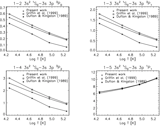
A sample of thermally-averaged collision strengths is shown in Fig. 2. For strong dipole-allowed transitions such as the reso-nance 1–5 line, we find vey good agreement between the calcu-lations. However, for several important transitions, we find gen-erally good agreement with the Griffin et al. (1999) values, but some differences with the Dufton & Kingston (1989) effective collision strengths for some transitions. However, as we shall see below, these differences do not significantly affect the intensities of the main diagnostic lines.
3.3. Line intensities
We have constructed an ion population model with our R-matrix collision strengths and A-values. We then calculated line inten-sities at log Ne [cm−3]=10 (a typical solar density) and log Te [K]=4.7, the temperature of maximum ion abundance in ioniza-tion equilibrium according to Dere et al. (2009) (but see the dis-cussion below). The calculated intensities of the brightest lines, relative to the resonance line (1–5, at 1206.5 Å), are listed in Table 3.
We also list (in brackets) the intensities calculated with the experimental A-value for the intercombination line, 1.67×10⁴ s−1by Kwong et al. 1983 instead of our value of 1.1×10⁴s−1. It is interesting to note that such large variation has a negligible effect on the intensity of the intercombination line, an issue that was pointed out by Jordan et al. (2001), but not noted by other studies on this ion. We have looked at the level population at log
Ne[cm−3]=10 and log Te[K]=4.7, corresponding to the relative intensities in Table 3. The 50% increase in the A-value for the intercombination line results in a similar decrease in the relative level population for the 3s 3p3P
1level, hence a similar line in-tensity, relative to the strongest 1–5 resonance line, which is not affected by the population of the 3s 3p3P
1 level. On the other hand, the population of several higher levels is significantly af-fected by direct excitation from the 3s 3p3P
1level, so a decrease in the population of the 3s 3p3P
1 level results in a decrease of the line intensities decaying from these levels. For example, the population of the 3p2 3P
0(No. 7) level is by about half due to di-rect excitation from the 3s 3p3P1, so it decreases by about 25%, which decreases the relative intensity of the 3–7 1301.1 Å transi-tion as shown in the table. In the ion model calculatransi-tions that we use in the rest of this paper, we adopt the experimental A-value for the intercombination line.
Regarding the important 5–15 transition at 1312.59 Å, we note that the upper level (3s 4s 1S
0) is mainly (by 84%) popu-lated by direct excitation from the ground state. Only about 10% of its population comes from excitations from the 3s 3p3P
j lev-els, and about 6% from radiative decays from upper levels. The 1312.59 Å line is the dominant decay from the upper level.
Table 3. List of the strongest Siiiilines.
i– j Levels I I g f Aji(s−1) Aji(s−1) Aji(s−1) λexp(Å)
CHIANTI Present CHIANTI N86
1–5 3s2 1S
0–3s 3p1P1 1.0 1.0 1.68 2.6×10⁹ 2.7×10⁹ 2.6×10⁹ 1206.50
1–3 3s2 1S0–3s 3p3P1 0.67(0.69) 0.50 1.8×10⁻⁵ 1.1(1.67)×104 1.5×10⁴ 1.8×10⁴ 1892.03
5–6 3s 3p1P
1–3p2 1D2 6.0(5.8)×10−2 5.8×10⁻² 0.13 2.6×10⁷ 2.4×10⁷ 3.1×10⁷ 2542.58
4–12 3s 3p3P
2–3s 3d3D3 5.1(4.9)×10−2 4.5×10⁻² 3.75 2.9×10⁹ 2.8×10⁹ 2.9×10⁹ 1113.23
4–9 3s 3p3P2–3p2 3P2 4.5(4.2)×10−2 3.5×10⁻² 2.11 1.7×10⁹ 1.7×10⁹ 1.7×10⁹ 1298.95
3–11 3s 3p3P
1–3s 3d3D2 1.7(1.5)×10−2 1.4×10⁻² 2.02 2.2×10⁹ 2.1×10⁹ 2.2×10⁹ 1109.97
3–9 3s 3p3P1–3p2 3P2 1.5(1.4)×10−2 1.2×10⁻² 0.71 5.6×10⁸ 5.7×10⁸ 5.6×10⁸ 1294.55
4–8 3s 3p3P
2–3p2 3P1 1.5(1.4)×10−2 1.1×10⁻² 0.70 9.2×10⁸ 7.7×10⁸ 9.1×10⁸ 1303.32
2–8 3s 3p3P
0–3p2 3P1 1.2(1.1)×10−2 9.2×10⁻³ 0.57 7.5×10⁸ 7.6×10⁸ 7.5×10⁸ 1296.73
5–16 3s 3p1P1–3s 3d1D2 1.1(1.1)×10−2 1.4×10⁻² 4.97 4.6×10⁹ 4.6×10⁹ 4.6×10⁹ 1206.56
2–10 3s 3p3P
0–3s 3d3D1 9.4(8.8)×10−3 7.6×10⁻³ 0.89 1.6×10⁹ 1.6×10⁹ 1.6×10⁹ 1108.36
3–8 3s 3p3P
1–3p2 3P1 8.9(8.4)×10−3 6.9×10⁻³ 0.42 5.6×10⁸ 5.7×10⁸ 5.6×10⁸ 1298.89
3–10 3s 3p3P1–3s 3d3D1 7.0(6.8)×10−3 5.7×10⁻³ 0.67 1.2×10⁹ 1.2×10⁹ 1.2×10⁹ 1109.94
5–15 3s 3p1P
1–3s 4s1S0 6.8(6.6)×10−3 7.4×10⁻³ 7.6×10⁻² 3.0×10⁸ 2.8×10⁸ 4.0×10⁸ 1312.59
4–13 3s 3p3P2–3s 4s3S1 6.2(5.9)×10−3 4.3×10⁻³ 0.57 1.3×10⁹ 1.3×10⁹ 1.3×10⁹ 997.39
4–11 3s 3p3P
2–3s 3d3D2 5.5(5.1)×10−3 4.5×10⁻³ 0.67 7.3×10⁸ 7.0×10⁸ 7.2×10⁸ 1113.20
3–7 3s 3p3P
1–3p2 3P0 4.6(3.7)×10−3 3.2×10⁻³ 0.56 2.2×10⁹ 2.3×10⁹ 2.2×10⁹ 1301.15
3–13 3s 3p3P1–3s 4s3S1 3.7(3.5)×10−3 2.6×10⁻³ 0.34 7.6×10⁸ 7.6×10⁸ 8.0×10⁸ 994.79
5–14 3s 3p1P
1–3p2 1S0 2.5(2.5)×10−3 1.9×10⁻³ 0.88 2.9×10⁹ 3.3×10⁹ 2.8×10⁹ 1417.24
12–19 3s 3d3D
3–3s 4p3P2 2.4(2.3)×10−3 1.4×10⁻³ 1.09 1.5×10⁸ 1.6×10⁸ 1.6×10⁸ 3087.13
6–20 3p2 1D2–3s 4p1P1 1.9(1.9)×10−3 1.5×10⁻³ 0.49 3.3×10⁸ 3.3×10⁸ 3.0×10⁸ 1842.55
6–27 3p2 1D
2–3s 4f1F3 7.6(7.5)×10−4 - 2.09 1.4×10⁹ - 1.7×10⁹ 1210.45
Notes. The first column lists the indices of the levels, as from Table 2. The second the spectroscopic notation. Column 3 shows the relative
intensities (photons) Int=NjAji/Neof the strongest lines, relative to the resonance transition, calculated at log Ne[cm−3]=10 and log Te[K]=4.7, using the level populations obtained with the present A-values and effective collision strengths. The values in brackets are the intensities obtained by assuming for the intercombination 1–3 line the experimental value of 1.67×10⁴. Column 4 shows the relative intensities obtained with the CHIANTI v.7.1 ion model. Column 5 lists our weighted oscillator strength g f , and column 6 our A-values. Column 7 lists the Dufton et al. (1983) A-values as given in the CHIANTI v.7.1 database, while column 8 those from Nussbaumer (1986) [N86]. All experimental wavelengths (λexp, last column) are in vacuum.
Fig. 2. Thermally-averaged collision strengths for a selection of transitions (see text).
an increased population, due to increased collision strength form the ground state (see Fig. 2).
Finally, we note that collisional data for the 3s 4f levels were not previously calculated. Sandlin et al. (1986) reports four lines as due to 3s 3d – 3s 4f transitions in Siiii, at 1210.45, 1500.23,
1501.187, and 1501.87 Å. We predict that the strongest transition is the 6–27 3p2 1D
[image:5.595.158.466.424.665.2]the observed ones, which casts doubts on the identifications of these lines in the solar spectrum.
4. Comparison with observations
The radiance of an optically thin transition is normally expressed as an integral along the line of sight
I(λji)=
Z
h
NeNHG(Ab,Ne,Te, λj,i) dh (1)
where λji is the wavelength of the transition, Ne, NH are the electron and neutral hydrogen number densities, and
G(Ab,Ne,T, λj,i) is the contribution function:
G(Ab,Ne,T, λi j)=Ab Aji hνi j
4π
Nj(Z+r) NeN(Z+r)
N(Z+r)
N(Z) (2)
which contains all of the relevant atomic physics parameters, and is mostly dependent on the electron temperature (for brevity, it is denoted below as G(T )). Aji is the spontaneous radiative transition probability, N(Z+r)/N(Z) is the relative ion popula-tion, Nj(Z+r)/N(Z+r) is the fractional population of the upper level, and Ab is the element abundance relative to hydrogen. The fractional level population is obtained by solving a system of equations taking into account all the excitation and deexcitation mechanisms.
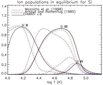
The ion population is normally obtained assuming equilib-rium conditions, and taking into account all ionization and re-combination rates. Several ion populations have been published over the years. Some are shown in Fig. 3. Most of them are obtained in the so-called low-density limit, whereby the den-sity dependence of the dielectronic recombination rates and the presence of metastable levels is neglected. In this case, Siiiiis
[image:6.595.70.285.521.699.2]relatively abundant in the range log T [K]=4.6–4.8. Arnaud & Rothenflug (1985) calculated the silicon ion populations by in-cluding charge transfer (CT) effects as they were described in Baliunas & Butler (1980). The addition of charge transfer shifts the peak of the Siiiiabundance to lower temperatures, about log T [K]=4.5, as Fig. 3 shows. We note that most of the other ion population tabulations do not include CT effects.
Fig. 3. Ion populations
Table 4 lists some of the quiet Sun observed intensities (de-scribed below) relative to the 1298.9 Å self-blend, as well as the
isothermal ratios calculated with the present atomic data, for dif-ferent temperatures. The relative intensity of the intercombina-tion line is in agreement with an isothermal temperature of about log T [K]=4.5, close to the peak of ion abundance suggested by Arnaud & Rothenflug (1985).
On the other hand, the relative intensity of the resonance line at 1206 Å is closer to the isothermal ratio at log Te[K]=4.7. Such discrepancies had been noted in previous literature, but the lower temperature was assumed to be correct (Dufton et al. 1984; Keenan et al. 1989; Pinfield et al. 1999). The assumption of an isothermal emission at log Te[K]=4.5 resulted in the intensity of the 1312.59 Å line being underestimated, which led to the intro-duction of non-Maxwellian electron distributions to explain the large intensity of the 1312.59 Å line.
The excitation energy of the transition (from the ground state) populating the upper level of the 1312.59 Å line is in fact significant (19.7 eV), much higher than that of the other lines ob-served nearby, so this line would be more sensitive to the high-energy tail of a non-Maxwellian electron distribution. Indeed Dufton et al. (1984) showed that, assuming a formation temper-ature of log Te[K]=4.5, the intensity of the 1312.59 Å line be-comes significantly enhanced in the non-Maxwellian case. This, according to the authors, provided plausible evidence for the
presence of non-Maxwellian electron distributions at the base of the transition region.
However, the isothermal approximation adopted by previous authors is not the correct approach, since the various Siiiilines
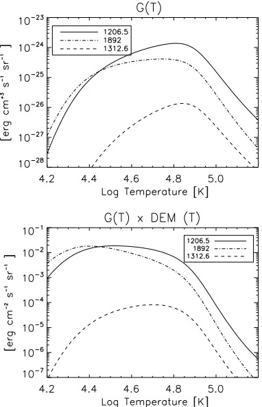
have a different temperature sensitivity. Fig. 4 (top) shows the contribution functions G(T ) for a selection of lines, obtained with the present level populations, the CHIANTI v.7.1 (Landi et al. 2013) ion population and the silicon photospheric abun-dance of Asplund et al. (2009). It is clear that the resonance and especially the intercombination line would mostly be produced by the lower-temperature layers of the solar atmosphere. It is well known that the plasma distribution in the lower transition-region has a very steep gradient, so to interpret the intensities of the Siiiilines, an understanding of the temperature structure
of the lower atmosphere for each observation is needed. This is normally done by assuming that a continuous distribution of the plasma at different temperatures exist, and estimating the col-umn differential emission measure (DEM) as a function of the electron temperature (from a set of selected transitions)
DE M(T )= NeNH
dh
dT [cm
−5K−1] . (3)
The DEM gives an indication of the amount of plasma along the line of sight that is emitting the radiation observed at a tempera-ture between T and T +dT . Such analysis is however often not
feasible for previous observations of Siiii lines, because lines
emitted from different ions were not reported.
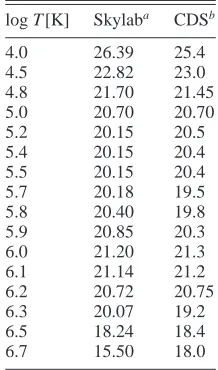
To illustrate the effect of the plasma distribution for the case of the quiet Sun, we have considered two quiet Sun DEM distri-butions. The first was obtained from SOHO CDS observations using older atomic data and the Arnaud & Rothenflug (1985) ion populations (Andretta et al. 2003). The values are tabulated in the Appendix. We have also obtained a second DEM from the Skylab observations of Vernazza & Reeves (1978), using for consistency recent atomic data, in particular the CHIANTI v.7.1 (Landi et al. 2013) ion populations. The details of the calcula-tions will be provided in a separate paper, while the DEM values are also tabulated in the Appendix.
Fig. 4 (bottom) shows the G(T )×DE M(T ) values using
intensi-Table 4. Ratios of observed and predicted QS line radiances
λ(Å) 1108 1109 1113 1206 1294.55 1296.73 1298.95+ 1301.15 1303.32 1312.6 1892 1298.89
Skylab (N77) - - - 17.8 0.28 0.20 1.0 0.10 0.34 0.08†
23.5
Skylab (N79) - - - 0.21 1.0 0.097 0. 0.12
-SUMER 0.25 0.38 0.92 37 0.29 0.22 1.0 - 0.41 0.16
-log Te[K]=4.7 0.20 0.52 1.14 18.47 0.28 0.22 1.0 0.12 0.27 0.10 7.8 log Te[K]=4.65 0.2 0.51 1.12 19.2 0.28 0.22 1.0 0.12 0.27 0.10 8.7 log Te[K]=4.6 0.18 0.49 1.05 21.51 0.28 0.22 1.0 0.12 0.27 0.08 11.6 log Te[K]=4.5 0.16 0.43 0.92 29.1 0.28 0.23 1.0 0.13 0.28 0.06 23.2 With QS DE Ma 0.18 0.49 1.06 24.8 0.28 0.22 1.0 0.12 0.27 0.09 19.5
With QS DE Mb 0.19 0.51 1.12 22.0 0.28 0.22 1.0 0.12 0.27 0.10 14.7
With QS DE Mc 0.17 0.46 0.99 29.2 0.28 0.22 1.0 0.12 0.28 0.08 28.8
With QS DE Md 0.18 0.49 1.06 25.7 0.28 0.22 1.0 0.12 0.27 0.09 22.6
Notes. The ratios (in energy units) are relative to the 1298.9 Å self-blend. The Skylab observed ratios are from Nicolas et al. (1977) [N77] and
Nicolas et al. (1979) [N79].†the 1312.6 Å measurement is from HRTS. The SUMER measurements are from Pinfield et al. (1999). We then list the
predicted ratios with the present atomic data, calculated at four temperature. The last four rows show the intensity ratios obtained by integration.
a: with the DEM obtained by Andretta et al. (2003) (see Appendix) and the CHIANTI v.7.1 ion population (Landi et al. 2013);b: with the DEM
obtained from the Skylab QS radiances of Vernazza & Reeves (1978) (see Appendix) and the CHIANTI v.7.1 ion population (Landi et al. 2013);c:
with the DEM obtained by Andretta et al. (2003) and the Arnaud & Rothenflug (1985) ion population;d: with the DEM obtained from the Skylab
[image:7.595.71.534.81.226.2]QS radiances of Vernazza & Reeves (1978) and the Arnaud & Rothenflug (1985) ion population.
Fig. 4. Top: contribution functions G(T ) for a selection of lines; bottom:
G(T ) values multiplied by the quiet Sun DEM obtained from Skylab
data.
ties of the lines are the integral of these curves over temper-ature. Table 4 lists the theoretical ratios obtained by integrat-ing G(T )×DE M(T ) with the two DEM distributions. Clearly,
all the lines that have the same temperature sensitivity as the 1298.9 Å line have isothermal ratios that are independent of
the temperature and are the same as those obtained by integrat-ing G(T )×DE M(T ). The 1312.59 Å line deviates, however its
isothermal ratio at log Te[K]=4.65 has the same value as that one obtained by integrating G(T )×DE M(T ), and is close to
the observed ratios. This means that the isothermal assumption with log Te[K] ≃ 4.65 is a reasonable approximation for the 1312.59 Å line, as well as the other lines around 1300 Å, in-cluding the resonance 1206.5 Å line.
Differences in the predicted ratios are found if different DEM distributions or ion populations (e.g. Arnaud & Rothenflug (1985) instead of the CHIANTI v.7.1) are used; however, with the exception of the intercombination line they are relatively small (within 20%), as shown in the Table. Therefore, the un-certainities related to the ion populations and the shape of the DEM distributions do not appear to affect our main conclusion, that the intensity of the 1312.59 Å line in the quiet Sun agrees with theory, without the need to invoke for the presence of non-Maxwellian distributions.
To simplify an overall comparison for all the lines, instead of showing how single line ratios behave as a function of den-sity or temperature as done in previous literature, we show the ’emissivity ratio’ curves, which are basically the ratios of the ob-served (Iob, energy units) and the calculated line emissivities as a function of the electron density Ne(or temperature Te):
Rji=
IobNeλji Nj(Ne,Te) Aji
C (4)
where Nj(Ne,Te) is the population of the upper level j relative to the total number density of the ion, calculated at a fixed temper-ature Te(or density Ne).λjiis the wavelength of the transition, Aji is the spontaneous radiative transition probability, and C is a scaling constant that is the same for all the lines within one observation. If agreement between experimental and theoretical intensities is present, all lines should be closely spaced or inter-sect, for a near isodensity (or isothermal) plasma. The value of
[image:7.595.74.265.339.635.2]electron density are similar to the L-function curves introduced by Landi & Landini (1997), the differences being that in the lat-ter case the observed intensities are divided by the line contribu-tion funccontribu-tions G(Teff), calculated at an effective temperature Teff,
which in turns depends on the differential emission measure. There are several solar observations of the UV lines, how-ever in may instances either the calibration of the instruments was uncertain, or the lines were not observed simultaneously, or only lines emitted over a narrow spectral range were observed. A selection of observations is discussed below.
[image:8.595.63.288.218.585.2]4.1. Skylab ATM observations
Fig. 5. Emissivity ratio curves relative to the quiet Sun Skylab ATM
observations 4′′inside the limb reported by Nicolas et al. (1977), with
the addition of an HRTS measurement of the 1312.59 Å line. Top: at a fixed log Ne[cm−3]=10.5; bottom: at a fixed log Te[K]=4.7. Iobindicates the measured intensity of a line in erg cm−2s−1sr−1.
We start by considering one of the very few published so-lar observations where both the resonance and the intercombina-tion lines were observed. The observaintercombina-tions were performed with the Naval Research Laboratory (NRL) EUV spectrograph on the Skylab Apollo Telescope Mount (ATM) and were reported by Nicolas et al. (1977). The slit was positioned at various loca-tions. In these and other subsequent observations, Siiiilines are
rather weak, unless the observations are close to the solar limb, so we have chosen the observation that was 4′′inside the limb,
although we note that the resonance line at 1206 Å has a large optical depth (see, e.g. Burton et al. 1971; Nicolas et al. 1977; Sandlin et al. 1986) at the limb.
The intensity of the weak 1312.59 Å line was not reported by these authors, so we have included a measurement that we have obtained for it from the HRTS observation described by Brekke et al. (1991). These authors published an excellent HRTS spectrum, obtained during the second rocket flight in February 1978. The spectrum was radiometrically calibrated by match-ing the quiet Sun intensities with those measured by the Skylab S082B calibration rocket flight CALROC. Variations between the HRTS and the CALROC were small, about±10%. The ab-solute calibration of the CALROC flight was ±25%. The long slit of the HRTS instrument scanned many solar regions, includ-ing the quiet Sun, plage, on disk and off-limb. We have anal-ysed these spectra and measured line intensities for a selection of regions. One of them is a quiet Sun region close to the solar limb, one of the few where the 1312.59 Å line was visible. We have chosen this region because the calibrated radiances of the nearby stronger lines were similar to those reported by Nicolas et al. (1977).
Fig. 5 (top) shows the corresponding emissivity ratio curves calculated at log Ne[cm−3]=10.5, and shows visually what we discussed above, i.e. that, with the exception of the resonance and intercombination lines, all the other lines have a similar tem-perature sensitivity. We have shown in Table 4 that good agree-ment (within a relative 20%) is found between all the observed and predicted radiances, taking into account a quiet Sun DEM distribution. The bottom plot of Fig. 5 shows the corresponding emissivity ratio curves at log Te[K]=4.7. A density of about log
Ne[cm−3]=10.5 provides good agreement for the lines observed around 1300 Å (No. 2 to 7). We note that the HRTS measure-ment of the 1312.59 Å line is in good agreemeasure-ment (within a rela-tive 20%) with the other lines.
Kjeldseth Moe & Nicolas (1977) provided Skylab ATM ob-servations close to the QS limb. The spectra were calibrated with a CALROC rocket flight which was calibrated on the ground, with typical uncertainties of 20%. We have considered a re-gion 12” inside the limb, because the same rere-gion was also ob-served by CALROC. The authors measured the intensities of the 1294.55, 1296.73, 1298.9, 1303.32, and 1892 Å lines. We find good agreement (to within 20%) with predicted intensities of the lines (they all have a similar density sensitivity), with the exception of the intercombination 1892 Å line, which is over a factor of three too bright with the isothermal assumption at log
Te[K]=4.7, as seen previously.
Dufton et al. (1983) reviewed older Skylab observations with the NRL slit spectrograph S082B, and provided some calibrated line ratios which we use here. They adopted a calibration pro-posed by Nicolas. Fig. 6 shows the emissivity ratio curves cal-culated at log Te[K]=4.7 relative to a quiet Sun and an active region observation, for a set of observed lines that have a similar temperature sensitivity. Excellent agreement (to within a±10%) is found, for densities of log Ne[cm−3]=10.1, 11.1 for the quiet Sun and active region, respectively.
men-Fig. 6. Emissivity ratio curves relative to the Skylab NRL slit
spectro-graph S082-B observations (Dufton et al. 1983). Iobindicates the mea-sured intensity of a line, normalised to the radiance of the 1296.73 Å line (energy units).
tioned, Dufton et al. (1984) pointed out that non-Maxwellian electrons would enhance the intensity of the 1312.59 Å line. Dufton et al. (1983) also suggested that perhaps the differences could be due to the temperature structure of the atmosphere, however the main uncertainity was related to the radiometric calibration of the Skylab NRL instrument, especially for the in-tercombination line (factor of two). However, we note that this would not explain the different discrepancies in different solar regions. Another problem with these Skylab observations is that lines were not recorded simultaneously.
4.2. HRTS observations
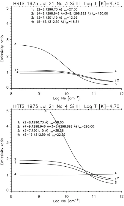
Nicolas et al. (1979) analysed a spectrum from a HRTS rocket flight on 1975 Jul 21. They used for the calibration the abso-lutely calibrated rocket spectrum of 1976 Oct 22. They provided calibrated intensities for four nearby lines in ten solar regions. The authors used older atomic data calculated with the DW ap-proximation, and reported significant discrepancies in the elec-tron densities obtained from different line ratios. On the con-trary, the present atomic data provide excellent agreement for all the lines. Fig. 7 shows the emissivity ratios calculated at log
[image:9.595.338.545.56.399.2]Te[K]=4.7, for two of the ten observations, relative to a quiet Sun (lower density) and an active region. The agreement is to within a few percent, i.e. is much better than the expected uncertainties
Fig. 7. Emissivity ratio curves relative to the HRTS rocket flight
spec-trum recorded on 1975 Jul 21, and regions No. 3, 4, relative to a quiet Sun and an active region (Nicolas et al. 1979). Iobindicates the mea-sured intensity of a line in erg cm−2s−1sr−1.
in the atomic data and instrument calibration. The intensity of the 1312.6 Å line is also in good agreement.
Keenan et al. (1989) analysed HRTS observations on 1985 Aug 1 aboard Spacelab 2, providing calibrated ratios of the 1296.73, 1301.15, 1303, and 1312.59 Å lines in three diff er-ent regions, a quiet Sun, an active region and a sunspot. The lines were recorded simultaneously. They also suggested that non-Maxwellian distributions may exist in all regions, because of the intensity of the 1312.59 Å line. On the other hand, with the present atomic data, we find good agreement between ob-served and predicted intensities at log Te[K]=4.7, the approx-imate formation temperature of these lines. We also note that the 1312.59 Å line was very weak (with significant blends in its wings), especially in the sunspot, so the measured intensity of this line is very uncertain.
[image:9.595.67.278.56.396.2]Fig. 8. Emissivity ratio curves relative to HRTS observations of a plage
and an umbra (Sandlin et al. 1986). Iobindicates the measured intensity of a line in erg cm−2s−1sr−1.
difficult to measure even in the HRTS spectra. In the plage, the observed intensity of this line is about a factor of two too weak compared to our predicted intensity, while in the umbra the op-posite is true, so we cannot reach any conclusions regarding the predicted intensity of this line.
4.3. SOHO SUMER observations
Pinfield et al. (1999) presented SOHO SUMER spectra of three solar regions, a coronal hole, a quiet Sun and an observation off
the limb, within an active region. They also suggested that non-Maxwellian distributions were present, an argument followed up by Dzifˇc´akov´a & Kulinov´a (2011).
The ratios of the quiet Sun values reported by Pinfield et al. (1999) are shown in Table 4, together with the Skylab+HRTS results. First, we note that the 1312.59 Å line is hardly visible in the coronal hole and quiet Sun data. Second, we note the un-usually high intensity of the 1206 Å resonance line, and of the 1303.32 and 1312.6 Å lines, while the 1294.55 and 1296.73 Å ratios are in good agreement. This casts doubts on the observed intensities, in particular in the measurement of the 1303.32 Å line. Third, we note that Pinfield et al. (1999) obtained, us-ing a combination of line ratios, log Te[K]=4.45 and log Ne [cm−3]=10.3 for the quiet Sun. As we have seen, the best line for density measurements is the 3–7 1301.15 Å one, which was not observed, so it is not possible to measure the density accurately, although the quiet Sun value suggested by Pinfield et al. (1999)
is in good agreement with previous results. The main problem is the low isothermal temperature obtained by Pinfield et al. (1999), which results in the observed intensity of the 1312.6 Å line be-ing about a factor of three higher than predicted, as we can see from Table 4.
As we have seen, estimating the line ratios by taking into ac-count a QS DEM distribution changes considerably the line ra-tios, and brings the relative intensity of the 1312.6 Å line within a factor of two the observed value.
Having said that, the intensity of the 1312.6 Å line in the off-limb AR observations of Pinfield et al. (1999) is indeed very high and at odds with the intensities of the other lines, so in that case the presence of a non-Maxwellian electron distribution is still a possible explanation. However, the SUMER lines were not observed simultaneously. The lower transition region lines are known to present strong variability on the shortest times ob-served, hence any non-simultaneous observations must be con-sidered with great caution.
5. Conclusions
We aimed first to test if some of the reported discrepancies be-tween observed and predicted Siiiiline intensities were due to
inaccuracies in the atomic data. We performed a new large-scale
R-matrix scattering calculation which provides line intensities
that are not largely different from those obtained from previous calculations. Variations are of the order of 20% so cannot explain the reported discrepancies.
Comparison with observation shows that the ratio of the 1301.15 Å line with any of the nearby lines is an excellent den-sity diagnostic that is largely independent of the temperature structure of the solar transition region. Ratios involving the res-onance and/or the intercombination lines can be used to mea-sure electron temperatures, if the plasma is nearly isothermal. However, for the lower solar atmosphere, where strong gradi-ents are present, understanding the Siiiispectrum is a complex
matter, since the resonance, and especially the intercombination line, are typically formed at lower temperatures than the other lines. Furthermore, the resonance line, having a large oscillator strength, is often affected by opacity effects.
We have reviewed all the Siiiimeasurements of the the 3s
3p 1P1–3s 4s 1S0 1312.6 Å line, since previous literature sug-gested that non-Maxwellian electron distributions were a pos-sible option to explain the intensity of this line. Clearly, sig-nificant uncertainties in the formation temperature of the Siiii
lines (i.e. ion populations) and the DEM distribution are present. However, they do not significantly affect the relative intensity of the 1312.6 Å line. By taking into account some example DEM distributions for the quiet Sun, we showed that the Siiiilines
around 1300 Å are effectively formed at similar temperatures (around log Te[K]=4.7 using the CHIANTI ion populations), so their ratio is not significantly affected by the thermal distribution of the transition region plasma.
We find in general very good agreement between the ob-served and predicted ratio of the 1312.6 Å line relative to the nearby lines. One exception are the SOHO SUMER observations (in particular the active region one), which are however uncer-tain, considering that lines were not observed simulaneously.
role in the formation of the Siiiilines. Future detailed modelling
(which is beyond the scope of the present paper) should take that into account, together with the temperature structure of the transition region.
The 1312.6 Å, as well as the 1417.2 Å line, is very weak and its predicted intensity depends significantly on the atomic structure. We have provided what we believe are the best atomic data for these lines, however further laboratory and astrophysi-cal measurements would be useful to confirm the present astrophysi- calcu-lations.
Acknowledgements. The present work was funded by STFC (UK) through the University of Cambridge DAMTP astrophysics consolidated grant, and the University of Strathclyde UK APAP network grant ST/J000892/1. This work is one of several on-going studies GDZ is carrying out to study non-Maxwellian electron distributions, within an ISSI team led by E. Dzifˇc´akov´a. We thank Carole Jordan for useful suggestions on how to improve the manuscript.
References
Andretta, V., Del Zanna, G., & Jordan, S. D. 2003, A&A, 400, 737 Arnaud, M. & Rothenflug, R. 1985, A&AS, 60, 425
Asplund, M., Grevesse, N., Sauval, A. J., & Scott, P. 2009, ARA&A, 47, 481 Badnell, N. R. 2011, Computer Physics Communications, 182, 1528
Badnell, N. R. & Gorczyca, T. W. 1997, Journal of Physics B Atomic Molecular Physics, 30, 2011
Badnell, N. R. & Griffin, D. C. 2000, Journal of Physics B Atomic Molecular Physics, 33, 2955
Baliunas, S. L. & Butler, S. E. 1980, ApJ, 235, L45
Baluja, K. L., Burke, P. G., & Kingston, A. E. 1980, Journal of Physics B Atomic Molecular Physics, 13, L543
Baluja, K. L. & Hibbert, A. 1980, Journal of Physics B Atomic Molecular Physics, 13, L327
Baluja, K. L., Kingston, A. E., & Burke, P. G. 1981, Journal of Physics B Atomic Molecular Physics, 14, 1333
Berrington, K. A., Eissner, W. B., & Norrington, P. H. 1995, Computer Physics Communications, 92, 290
Brekke, P., Kjeldseth-Moe, O., Bartoe, J.-D. F., & Brueckner, G. E. 1991, ApJS, 75, 1337
Burke, P. G. & Robb. 1975, Adv.At.Mol.Phys., 11, 143
Burton, W. M., Jordan, C., Ridgeley, A., & Wilson, R. 1971, Royal Society of London Philosophical Transactions Series A, 270, 81
Del Zanna, G. 1999, PhD thesis, Univ. of Central Lancashire, UK
Del Zanna, G., Dere, K. P., Young, P. R., Landi, E., & Mason, H. E. 2014, A&A, in prep.
Del Zanna, G., Landini, M., & Mason, H. E. 2002, A&A, 385, 968
Del Zanna, G., Storey, P. J., Badnell, N. R., & Mason, H. E. 2012, A&A, 541, A90
Dere, K. P., Landi, E., Mason, H. E., Monsignori Fossi, B. C., & Young, P. R. 1997, A&AS, 125, 149
Dere, K. P., Landi, E., Young, P. R., et al. 2009, A&A, 498, 915
Dufton, P. L., Hibbert, A., Kingston, A. E., & Doschek, G. A. 1983, ApJ, 274, 420
Dufton, P. L. & Kingston, A. E. 1989, MNRAS, 241, 209 Dufton, P. L., Kingston, A. E., & Keenan, F. P. 1984, ApJ, 280, L35 Dzifˇc´akov´a, E. & Kulinov´a, A. 2011, A&A, 531, A122
Eissner, W., Jones, M., & Nussbaumer, H. 1974, Computer Physics Communications, 8, 270
Fern´andez-Menchero, L., Badnell, N. R., & Del Zanna, G. 2014, A&A, 0, in prep
Griffin, D. C., Badnell, N. R., & Pindzola, M. S. 1998, Journal of Physics B Atomic Molecular Physics, 31, 3713
Griffin, D. C., Badnell, N. R., Pindzola, M. S., & Shaw, J. A. 1999, Journal of Physics B Atomic Molecular Physics, 32, 2139
Hibbert, A. 1975, Computer Physics Communications, 9, 141
Hummer, D. G., Berrington, K. A., Eissner, W., et al. 1993, A&A, 279, 298 Jordan, C., Sim, S. A., McMurry, A. D., & Aruvel, M. 2001, MNRAS, 326, 303 Keenan, F. P., Dufton, P. L., Kingston, A. E., & Cook, J. W. 1989, ApJ, 340, 1135 Kjeldseth Moe, O. & Nicolas, K. R. 1977, ApJ, 211, 579
Kramida, A., Ralchenko, Y., & Reader, J. 2013, 0
Kwong, H. S., Johnson, B. C., Smith, P. L., & Parkinson, W. H. 1983, Phys. Rev. A, 27, 3040
Landi, E. & Landini, M. 1997, A&A, 327, 1230
[image:11.595.381.490.79.264.2]Landi, E., Young, P. R., Dere, K. P., Del Zanna, G., & Mason, H. E. 2013, ApJ, 763, 86
Table A.1. Column quiet Sun DEM used here
log T [K] Skylaba CDSb
4.0 26.39 25.4 4.5 22.82 23.0 4.8 21.70 21.45 5.0 20.70 20.70 5.2 20.15 20.5 5.4 20.15 20.4 5.5 20.15 20.4 5.7 20.18 19.5 5.8 20.40 19.8 5.9 20.85 20.3 6.0 21.20 21.3 6.1 21.14 21.2 6.2 20.72 20.75 6.3 20.07 19.2 6.5 18.24 18.4 6.7 15.50 18.0
Notes.a:DEM obtained from the Skylab QS radiances of Vernazza &
Reeves (1978) and the CHIANTI v.7.1 ion populations (Landi et al. 2013);b: DEM obtained by Andretta et al. (2003) from SOHO CDS
quiet Sun radiances and the Arnaud & Rothenflug (1985) ion popula-tions.
Laughlin, C. & Victor, G. A. 1979, ApJ, 234, 407
Livingston, A. E., Baudinet-Robinet, Y., Garnir, H. P., & Dumont, P. D. 1976a, Journal of the Optical Society of America (1917-1983), 66, 1393
Livingston, A. E., Kernahan, J. A., Irwin, D. J. G., & Pinnington, E. H. 1976b, Journal of Physics B Atomic Molecular Physics, 9, 389
Nicolas, K. R., Bartoe, J.-D. F., Brueckner, G. E., & Vanhoosier, M. E. 1979, ApJ, 233, 741
Nicolas, K. R., Brueckner, G. E., Tousey, R., et al. 1977, Sol. Phys., 55, 305 Nussbaumer, H. 1986, A&A, 155, 205
Ojha, P. C., Keenan, F. P., & Hibbert, A. 1988, Journal of Physics B Atomic Molecular Physics, 21, L395
Pinfield, D. J., Keenan, F. P., Mathioudakis, M., et al. 1999, ApJ, 527, 1000 Reisenfeld, D. B., Gardner, L. D., Janzen, P. H., Savin, D. W., & Kohl, J. L.
1999, Phys. Rev. A, 60, 1153
Sandlin, G. D., Bartoe, J.-D. F., Brueckner, G. E., Tousey, R., & Vanhoosier, M. E. 1986, ApJS, 61, 801
Saraph, H. E. 1978, Computer Physics Communications, 15, 247 Seaton, M. J. 1975, Adv.At.Mol.Phys., 11, 83
Strong, K. 1978, PhD thesis, University College London, UK Vernazza, J. E. & Reeves, E. M. 1978, ApJS, 37, 485
Victor, G. A., Stewart, R. F., & Laughlin, C. 1976, ApJS, 31, 237 Wallbank, B., Djuri´c, N., Woitke, O., et al. 1997, Phys. Rev. A, 56, 3714
Appendix A: Quiet Sun DEM from Skylab ATM observations