Interception and deviation of near Earth objects via solar collector strategy

IAC-08-A3.I.06

INTERCEPTION AND DEVIATION OF NEAR EARTH OBJECTS

VIA SOLAR COLLECTOR STRATEGY

CAMILLA COLOMBO

PhD Candidate, Department of Aerospace Engineering, University of Glasgow, UK, [email protected]

MASSIMILIANO VASILE

PhD, Department of Aerospace Engineering, University of Glasgow, UK, [email protected]

GIANMARCO RADICE

PhD, Department of Aerospace Engineering, University of Glasgow, UK, [email protected]

ABSTRACT

A solution to the asteroid deviation problem via a low-thrust strategy is proposed. This formulation makes use of the proximal motion equations and a semi-analytical solution of the Gauss planetary equations. The average of the variation of the orbital elements is computed, together with an approximate expression of their periodic evolution. The interception and the deflection phase are optimised together through a global search. The low-thrust transfer is preliminary designed with a shape based method; subsequently the solutions are locally refined through the Differential Dynamic Programming approach. A set of optimal solutions are presented for a deflection mission to Apophis, together with a representative trajectory to Apophis including the Earth escape.

1.

INTRODUCTION

he ongoing panel discussion about asteroids aims at assessing the level of technology to detect, track, study and deviate potentially dangerous near Earth objects. Among the possible responses to an asteroid impact hazard, different deviation techniques have been identified, whose interaction with the asteroid can produce an impulsive change of its linear momentum (e.g. kinetic impactor, nuclear explosion) or a continuous momentum change by a low-thrust applied to the object (e.g. electrical/chemical engines or solar sails anchored to its surface, gravity tractor, mass drivers, solar collector, pulsed laser, enhanced Yarkovsky effect) [1]. One strategy would be to produce a sublimation of the surface material through

a laser beam or a solar concentrator. This deflection strategy exploits the benefits of a slow-push technique and makes use of a free power source.

In order to have an effective and efficient mitigation scheme, the total mass of the spacecraft into orbit and the warning time should be minimal for a given deviation. An optimal solution can be obtained by the integrated design of the interception phase (transfer from the Earth to the asteroid) and the deflection phase.

masses into space. Instead of using a single hypothetical mission case, a set of hundreds of solutions is found, each one representing a complete mission with a specific launch date and transfer time. Fixed the dry mass of the spacecraft at the asteroid interception, a set of Pareto optimal points is found according to three criteria: the achievable displacement of the asteroid at the point of Minimum Orbit Interception Distance (MOID), the time between the launch and the hypothetical impact and the propellant mass for the transfer trajectory. Reconstructing the set of all Pareto optimal solutions requires the evaluation of several tens of thousands of trajectories, thus the numerical computation of the low-thrust transfer trajectory of the spacecraft and of the deflected trajectory of the asteroid would be impractical.

Since 1950 several authors have proposed analytical solutions to some particular cases of the low-thrust problem [3]-[7]. Kechichian [8] used an averaging technique to compute analytical solutions for orbit raising with constant tangential acceleration in the presence of Earth shadow, also considering the effects of the Earth oblateness. Gao and Kluever [9] adopted an averaging technique with respect to the eccentric anomaly, for continuous tangential thrust trajectories; the accuracy of their solution depends on the eccentricity.

Other analytical solutions for low-thrust trajectories were studied by Petropoulos [10] who developed some analytical integrals to describe the secular evolution of the orbit of a spacecraft, subject to different thrust control laws. The rate of change of the orbital energy and the eccentricity are time-averaged and reformulated introducing some elliptic integrals, which are valid for all initial eccentricity from slightly above zero.

This paper uses a semi-analytical approach [11] to compute the displacement of the position of an asteroid at the MOID point, after a low-thrust deviation manoeuvre. The miss distance achieved with a given deviation action is computed analytically by means of the proximal motion equations [12],[13] expressed as a function of the orbital elements. The variation of the orbital

parameters is then computed through Gauss’

planetary equations [14]. Note that the computation of the miss distance through the proximal motion equations can be adopted for any deviation strategy and represents an extension and a generalization of the methodologies proposed in previous works [15]-[17] in which analytical formulae were derived to compute the deviation due to a variation in the orbital mean motion.

The assumption for the analytical developments used in this paper is that the deflection strategy uses

the Sun as a power source and therefore the thrust acceleration is inversely proportional to the square of the distance from the Sun. Furthermore, we focus our attention on the case in which the thrust is aligned with the tangent to the osculating orbit of the asteroid.

In order to obtain an analytical solution for the variation of the orbital elements, Gauss’ equations are averaged over one orbital revolution. However, the required accuracy for the computation of the miss distance is higher than for the design of a generic low-thrust trajectory, hence, unlike other works [8]-[10], also the periodic variation of the orbital elements is taken into account. In addition, the analytic integrals are updated with a one-period step to further improve the accuracy.

The preliminary design of the low-thrust trajectory is performed through a shape based approach [18], which provides an estimation of the required propellant mass. As a second stage, an algorithm based on the Differential Dynamic Programming [19]-[21] is adopted for the refinement of the transfer solutions. This successive approximation technique applies recursively,

backwards in time, Bellman’s principle of optimality

in the neighbourhood of the nominal trajectory, finding an improved control law. In this way the large scale problem associated with the optimisation of a low-thrust trajectory is translated into a series of problems of small dimensions.

Finally this paper presents a family of optimal solutions for a potential deflection mission to asteroid Apophis.

2.

ASTEROID DEVIATION PROBLEM

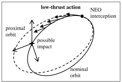
Given the time of interception ti of a generic

Fig. 1 Slow-push deviation strategy.

If  is the true anomaly of the NEO at the MOID along the unperturbed orbit and *_{ } 

the corresponding latitude, we can write the variation of the position of the NEO, after deviation, with respect to its unperturbed position by using the proximal motion equations:













2 3 2 * * sin cos 1 cos sin

2 cos cos

sin cos sin r

h

r ae

s a M a e

a r

s e M r

r

e e r i

s r i i

             _{  }                     (1)

where s_r, s and sh are the displacements in the

radial, transversal and perpendicular to the orbit plane directions respectively, so that the deviation is





T

r h

s s s

r    , and 2

1 e

   . In a matrix form:



tMOID



MOID

r A  (2)





T

a e i M

        is the vector of

the orbit element difference at the MOID between the perturbed and the nominal orbit, where M is the mean anomaly. When a slow-push deviation action is applied over the interval



ti te



, being tetMOID the

time when the manoeuvre is ended, the total variation of orbital parameters is computed by integrating

Gauss’ planetary equations:





2 * * * 2 2 1

2 cos sin

cos

sin sin 1

2 sin 2 cos

sin cos sin

2 1 sin cos

t t n h h t n h t n

da a v a dt

de r

e a a

dt v a

di r a

dt h

d r

a

dt h i

d r

a e a

dt ev a

r i

a h i

dM b e r r

n a a

dt eav p a

      _{ }        _   _           _ _  _{ }            _{ }  _  _     (3)

The slow-push strategy provides an acceleration

 





T

t n h t  a a a

a , here expressed in a

tangential-normal-binormal reference frame, such that a_t and

n

a are the components of the acceleration in the plane of the osculation orbit, along the velocity vector and perpendicular to it. Note that the derivative of M, in the 6th equation of system (3), takes into account the instantaneous change of the orbit geometry at each instant of time t



ti te



and

the variation of the mean motion due to the change the semi-major axis on the thrust arc.

Said

 

t 



a e i   M



T the vector of the orbital parameters, we define:

   





e i

T

t t

a e i  M

   

      

the finite variation of the orbital elements with respect to the nominal orbit, in the interval



ti te



,

obtained form the numerical integration of Eqs. (3). It is important to point out that   a a,   e e,

i i

[image:3.612.79.282.70.206.2]

 





 

















MOID e e MOID e

i e MOID e

i i p e MOID e

MOID i MOID p

M M t n t t

M t M n t t

n t t M n t t

M n t t

   

     

     

 



where t is the passage at the pericentre, we can p

conclude that the total variation in mean anomaly between the proximal and the unperturbed orbit is:



eMOIDi



MOIDMOID i i e e

M M M

n n t n t n t M

   

    



(4)

where ni is the nominal angular velocity and





3

e n

a a

 

  .

At this point Eqs. (1) can be used to compute the consequent r.

2.1.

Analysis of the Optimal Thrust

Direction

An estimation of the optimal thrust direction [11] of the push can be obtained by maximising the deviation r at the MOID, given the time-to-impact  t



tMOIDti



. The deviation vector can be

computed as:



tMOID



MOID t

 

t

 

t

r A G v T v

where T is the transition matrix that links the impulsive v at time t to the consequent deviation at t_MOID. A_MOID is the matrix in (2) and G_t is the matrix associated to the Gauss’ equations written for finite differences, i.e. the control acceleration being replaced by an instantaneous change in the asteroid velocity vector:

 

t t

 G v

Following Conway’s [22] approach, r can be maximised by choosing an impulse vector vopt

parallel to the eigenvector of conjugate to the maximum eigenvalue. As a result of this analysis, we

can derive that for a ∆t larger than a specific tNEO

smaller than the nominal period of the asteroid TNEO,

the optimal impulse presents a dominant component along the tangent direction, being this one associated to the shifting in time between the position of the asteroid and the Earth, rather than to a geometrical variation of the MOID. This conclusion is in agreement with previous works [22]-[24]. In the case of a low-thrust manoeuvre, as a first approximation, this results can be generalized by choosing the control vector at time t instantaneously tangent to the optimal impulsive v t . Hence in this work, we focus on low-thrust acceleration in the tangent direction. This is a valid assumption when we consider hazardous cases with a warning time longer than approximately 0.75TNEO.

3.

SEMI-ANALYTICAL FOMULAE

FOR LOW-THRUST DEVIATION

ACTIONS

A set of semi-analytical formulae [11] were derived to calculate the total variation of the orbital parameters due to a low-thrust action. It is considered that a continuous acceleration at is applied along the

orbit track, with modulus given by:

2 t

k a

r

 (5)

Where r is the distance from the Sun and k is a time-invariant proportionality constant that has to be fixed according to the specification of the power system. The selection of this acceleration law does not represent a severe restriction to the mission design, in fact Eq. (5) describes any strategy that exploits the Sun as a power source, e.g. a solar electric propulsion spacecraft that rendezvous with the NEO, anchors to its surfaces and pushes, or a solar mirror which collects the energy from the Sun and focuses it onto the asteroid surface to ablate it. Moreover, if the formulae presented in the following are adopted to design a low-thrust trajectory, Eq. (5) represents the control acceleration due to a power-limited spacecraft.

Gauss’ equations are written as a function of the true latitude:

* *

d d dt

dt

d  d (6)

where

*

2

d h

dt r



 . Eqs. (6) are averaged over one

,2 2 * * 0 1 2 d d d d d       





The total variation of the orbital elements over one orbital period of *

can be approximated as:

,2 2 * 0 d d d       



if a zero variation in the anomaly of the pericentre is assumed, i.e. d*d. This assumption holds true in the case the deviation is calculated over an integer number of orbital revolutions, because the periodic variation of  is zero and the secular one is of order

11

10 . The analytical formulae derived after some algebraic manipulations are:



_{  }





















0 0 0 0 0 0 0 0 0 0 2 2 2 2 , 2 2 , 2 , 2 , 1 2 4

1 E ,

2 ₁

4

1 F ,

2 ₁

4 2 E ,

2 1 2

0

0

1 2 cos

2 1 2 arctan 1 e e e e e e e k e e e

h ev _e

e e e e v e a k a h i e e k eh ev e M                        _             _ _  _                        _  _                            0 0 0 0 2 2 2 , 2 2 , tan 2

1 sin 2 1 2 cos

1 cos

2 arctan 1 2 cos

1

e e

e e

e e bk e e

e eah ve

v a e e e v e              _{  }  _{  }_             _   _             _    _  _ (7)

where v is the orbital velocity and  is defined as:

 





2

2

1 2 cos

1 e e e       

Eqs. (7) contain two elliptic integrals to be evaluated only once every orbital period: F is the incomplete elliptic integral of the first kind and E the incomplete elliptic integral of the second kind [14],[25]. Note that the integral kernels (7), to be evaluated in 02 and 0, are function only of the

semi-major axis and the eccentricity.

The variation of the mean anomaly M strongly influences the consequent deviation, calculated through Eqs. (1). Hence, in order to have a better approximation of M in Eqs. (7), the value of the eccentricity is updated in the evaluation of the integral kernels. This allows taking into account the secular variation e over one orbital revolution.

Finally, the total variation of the orbital parameters over the thrust arc is determined by integrating Eqs. (7) with the Euler method with a step of one orbital period.

The analytical formulation in Eqs. (7) describes the mean variation of the Keplerian elements, hence it gives a sufficiently accurate estimate of their variation over one full revolution of the true latitude. For smaller angular intervals, the periodic component of the perturbation must be included because its variation is not zero. To this aim, an expression was derived to estimate the periodic component of semi-major axis, eccentricity and argument of the perigee.

The trend of a , e ,  function of *

can be approximated by the following equations:

 

_

_









 

_

_









 

_

_









* * * 0 0 * * * * 0 * * * 0 0 * * * * 0 * * * 0 0 * * * * 0 sin sin 2 sin sin 2 cos cos 2 a p a p e p e p p p

a a C

a

C

e e C

e C C C                                                         (8)

The first two terms in Eqs. (8) are the initial condition for the secular variation of the orbital parameters at point 0 (i.e. the point when the deviation action commences), the third term indicates the secular variation obtained form Eqs. (7) and the forth one is the periodic variation. The coefficients

a

C , Ce and C are the amplitudes of the periodic

of the perturbation is almost constant over a sufficient number of integration periods (i.e. needed to deviate the asteroid of a considerable safe distance).

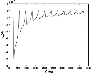
For example, Fig. 2 compares the semi-analytical expression of the eccentricity (continuous bold line) to the numerical one (continuous normal line) for asteroid Apophis. The dot line represents the mean variation.

Fig. 2 Analytic expression of the eccentricity. Asteroid Apophis.

In order to properly take into account the periodic variation of the mean anomaly within an interval smaller than one revolution, the corresponding

Gauss’ equation has to be integrated over *

:

2 2

* 2 1 sin t

dM b e r r

n a

eav p h

d 

   

_  _  _{ }

 

  (9)

in which

 

*

e  ,

 

*

a  and  

 

*

are expressed through Eqs. (8).

3.1.

Accuracy Analysis

The accuracy of Eqs. (7) was assessed by computing the relative error on the achieved deviation r between the numerical propagation of

Gauss’ equations and the analytical formulae:

propagated analytical r

propagated

e  

 

 r r

r .

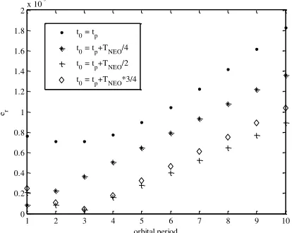
Fig. 3 represents the relative error for the deviation of asteroid 1979XB, pushing over an increasing number of orbital revolutions and starting the deviation manoeuvre at different angular positions. In fact the variation of the orbital parameters over one orbital revolution depends on

where, along the orbit, the manoeuvre starts. In the legend tp is the time at the pericentre, t0 the time

when the deviation action commences and TNEO is the

asteroid nominal orbital period. An adaptive step-size Runge-Kutta Fehlberg integrator was used, setting the absolute and the relative tolerance respectively to

16

1 10  and 2.3 10 14 in order to obtain a relative error of 105.

1 2 3 4 5 6 7 8 9 10 0

0.2 0.4 0.6 0.8 1 1.2 1.4 1.6 1.8

2x 10 -5

orbital period

er

t₀ = t_p t₀ = t_p+T_NEO/4 t₀ = t_p+T_NEO/2 t₀ = t_p+T_NEO*3/4

Fig. 3 Relative error on the deviation. Asteroid 1979XB.

Fig. 4 to Fig. 6 present the relative error between semi-analytical expression and numerical values of e, a,  for asteroid 1979XB and the relative error on M with respect to the full integration of Eqs. (6) is depicted in Fig. 7. The analysis of the accuracy of the formulae was performed on different orbits, to verify the sensitivity to the orbital elements.

[image:6.612.72.287.166.327.2] [image:6.612.329.536.193.358.2] [image:6.612.333.523.506.664.2]

Fig. 5 Relative error between the numerical and semi-analytical expression of the semi-major axis. Asteroid 1979XB.

Fig. 6 Relative error between the numerical and semi-analytical expression of the anomaly of the pericentre. Asteroid 1979XB.

Fig. 7 Relative error between the numerical and semi-analytical expression of the mean anomaly. Asteroid 1979XB.

4.

TIME FORMULATION

The approach described in paragraph 3, which will be referred to in the following as latitude formulation, does not make use of the time as a variable to describe the perturbed motion.

However the time is required when dealing with the asteroid deviation problem since the component of the deviation associated to the shift in time has to be taken into account. In fact the latitude formulation accounts only for the shift in position of the asteroid. Given the thrust arc



ti te



we want to apply the

semi-analytical formulation described in order to find the displacement of the asteroid after a certain time.

Eqs. (7) are used to compute the variation of the orbital elements over the number of full revolutions contained in the time interval



ti te



. Whereas, for

the remainder of the thrusting arc, the element differences are calculated using Eqs. (8) and (9). The interval *

corresponding to the time interval



ti te



is computed by numerically integrating Eq.

*

2

d h

dt r

 _

. Note that the terms corresponding to the

secular variation of the parameters in Eqs. (8) are calculated updating a, e and  at each orbital revolution.

4.1.

Accuracy Analysis

The accuracy of the time formulation algorithm was verified. The deviation ranalytical tf, achieved

pushing over an increasing interval was calculated trough the algorithm summarised in section 4 and the result was compared with the deviation rpropagated tf,

computed with the numerical integration of Eqs. (3),

Gauss’ equations function of time.

, ,

,

, propagated tf analytical tf r time formulation

propagated tf

e  

 

 r r

r

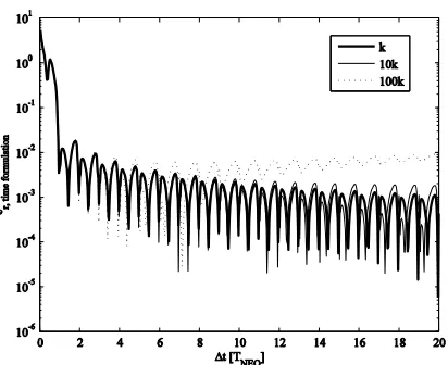
The relative error was computed for increasing values of the proportionality constant k. Fig. 8 reports

,

r time formulation

e calculated with the nominal value of k (set in section 6), 10k and 100k, for asteroid 1979XB. The values of er time formulation, are plotted against the

push time teti, which was set equal to the

[image:7.612.83.271.74.231.2] [image:7.612.81.275.287.439.2] [image:7.612.85.276.493.648.2]

Fig. 8 Relative error of the time formulation. Asteroid 1979XB (k=2·104 km3/s2).

The high value of the relative error when 1NEO

t T

  is due to the approximation introduced with the periodic component of the orbital elements in Eqs. (8). For  t 1TNEO the element difference

between the perturbed and the nominal orbit  is of the same order of magnitude of the approximation error of the periodic component; moreover the secular variation is still small. As a consequence the relative error on the elements difference

  , ,

, propagated tf analytical tf r

propagated tf

e   

  

is high. In particular this affects the difference of mean anomaly which significantly contributes to the terms in Eqs. (1). For this reason, the time formulation can be substituted to the numerical integration for a thrust arc t longer than one orbital revolution. On the other hand, we need to consider that when low-thrust strategies are selected, the thrust arc is in general longer than 1 TNEO.

Finally Fig. 9 depicts the percentage of saving in computational time of the semi-analytical approach, with time formulation, with respect to the numerical integration. When  t 1TNEO the gain is around the

40% and it increases with the length of the push arc.

Fig. 9 Percentage of saving in computational time by using the semi-analytical time formulation with respect to the numerical integration of Gauss’ equations. Asteroid 1979XB.

5.

DIFFERENTIAL DYNAMIC

PROGRAMMING

For the global search a hybrid optimisation approach was used [2],[26], which blends a stochastic search with an automatic solution space decomposition technique. Each point of the Pareto set is a complete mission, composed by two phases; the first leg is a low-trust transfer, from the Earth to the rendezvous with the asteroid and after that the deflection phase is performed. The achievable displacement of the asteroid at the point of MOID pushing over a time interval t is computed trough the time formulation of the semi-analytical approach (section 4). The transfer trajectory, instead, was calculated through a shape-based method [18],[27]. The low-thrust transfer is computed in the two body problem, assuming zero velocity at the Earth sphere of influence. Moreover a 25% of margin was added to the spacecraft mass at launch.

As a second stage, in order to improve our analysis, we performed a local optimisation of the low-thrust trajectories.

The design of low-thrust trajectories requires the solution of an optimal control problem, the difficulty of which increases with the complexity of the dynamics. The low level of thrust implies long transfer times and moreover variable times and distances scales are introduced (for example when we consider the Earth escape and the heliocentric leg).

[image:8.612.324.537.76.235.2] [image:8.612.79.285.77.245.2]

other approaches, the time dependence is not removed from the parameterisation. It satisfies

Bellman’s principle of optimality so its solution should be as accurate as the solution of indirect methods, and unlike those it does not require a first guess for the Lagrange multipliers.

The DDP is a successive approximation technique; in each iteration, given the current nominal trajectory and control, some auxiliary equations are integrated backward in time, giving the coefficients of the linear/quadratic approximation of the cost function, in the neighbourhood of the nominal trajectory and an improved control policy is computed. The trajectory is then forward integrated with the new control law and the reduction of the cost function is verified. Hence the control becomes the nominal policy for the next iteration. By several iterations a control strategy is determined, which progressively approximates the optimal control law.

The standard DDP works with two variable classes: the state vector s t

 

, composed by position, velocity and mass of the spacecraft at time t and the dynamic control vector u t

 

that in our specific case is the low-thrust provided by the engine.

For each iteration the optimisation is discretised in N stages that represent the decision times of the trajectory. These stages can be identified as the integration steps for the discrete time dynamic of the problem:





1

1 1

, ; 1,....,

  



j j j j

s f s u t j N

s s

where the state transition function f comprehends the dynamics equations and the integration scheme. In our case a Runge-Kutta Fehlberg scheme of the 4th order was used.

The cost function of a trajectory with initial condition s1 and control schedule

 

uj is

 



1









1 1



1

; ,  _; _







N  T

j j j N N

j

J u s g s u b s t

where the first term represents the integral term function of



x uj, j



and the second term introduces

the terminal constraints of the form 



sN1;tN1



0,

multiplied by a time invariant set of Lagrange multipliers b.

For our problem we set the integral cost function to be a quadratic function of the thrust vector T, with a weight matrix R and the integration step

1



 

j j j

h t t , while the terminal constraints represents the condition of rendezvous with the asteroid:





2

1 target 1

1 _ˆ

2 







N T  T 

j j j N j

J T RT h b s s (10)

The DDP bases on Bellman principle of optimality. At the stage j we define the optimal return function

 

min 



, ;



 1

 

1 

j

j j j j j j j

u

V s g s u t V s (11)

as the cost due to initial condition s if the optimal _j policy is employed. The DDP applies the principle of optimality (dynamic programming) in the neighbourhood of a nominal trajectory, so at each stage j the cost function and the optimal return function from the next stage onward are replaced by their quadratic approximation (QP) about the current nominal control and trajectory (the superscript dash indicates the nominal conditions):















1 1 1



min , ;

j

j j j

j j j j j j j j u

V s s

QP g s s u u t V s s



  _{ }  _

 

   

 

 

(12)

with the initial condition









1 1  1; 1

   T  

N N N N

V s b s t

The minimisation in Eq. (12) is performed from the final stage N+1 until stage 1. The main requirement for the assumption of the quadratic approximation to hold true is that the variations in the state from the nominal state due to the new control sequence should be sufficiently small. This may be achieved even if the variation in the control action is large, provided that the time duration of this variation is small. In this work we implemented an optimisation algorithm that employs global variations in the control [19]. The main core of the DDP algorithm is composed by two phases: a backward and a forward propagation.

The first recursion is performed backward in time, stagewise form state N+1 to state 1.





 

*

*

1 1 min _  , ,     _

j

j j j j j

u QP g s u t QP V s

(13)

In our case the minimisation of Eq. (13) was performed through a sequential quadratic programming method. Then the linear/quadratic expansion of the cost and return function is computed, about the point



*



, j j

s u . The coefficients

of the Taylor expansion are explicitly written in term of the first and second derivatives of the state transition function, the stagewise loss function and the optimal return function form the stage onward. This allows the construction of the coefficient j

determining the feedback strategy, which is stored in memory for the forward recursion. The algorithm has quadratic convergence under the assumption that the Hessian matrix of the cost function is positive definite. In the other cases a shift procedure on the eigenvalues of the matrix is employed to make them positive [20].

The forward recursion starts with the initial condition s1. The change in control uj j sj

from * j

u is function of the state variation and the coefficients computed in the backward recursion. The successor policy u is constructed and the new _j trajectory is propagated through the state transition function f:





*

1

1,..., ( , ; )





    

 _

  

j j k j j

j j j j

u u s s

j N

s f s u t

A step size adjustment procedure ensures that the variation of the control does not break the assumption of the linear/quadratic approximation. So the corrected strategy will be:





lim

*

lim 1,...,

,...,



 



 _{    }



j j

j j j j j

u u j j

u u s s j j N

The nominal control is applied from the initial step to a step jlim and after that the new strategy is

adopted. This scheme allows for an improvement in the value cost function J

 

 

u_j with respect to its nominal value of the previous DDP iteration:

 

 

j 

 

 

j  

 

lim

J u J u c j

where 

 

j_lim is the expected hypothetical gain in the case the right term of Eq. (11) was quadratic.

The successive iteration of backward and forward recursions continues until a convergence criterion is satisfied. Note that in this phase the value of Lagrange multipliers is kept constant.

The equality constraints on the final state are handled through an external phase of DDP as suggested by Gershwin and Jacobson [28]. A variation of the Lagrange multiplier b and a proportional variation of the control are computed, in order to decrease the constraints violations . In this way the control strategy is modified to:

1,..., j j j j

b b b

u s b j N

 

     

  

     

where j is a coefficient computed backward in time

by expanding Eq. (12) also in the neighbourhood of b , and 0  1 ensures that 



sN1;tN1



is

reduced.

[image:11.612.86.272.75.500.2]

Fig. 10 DDP algorithm.

The principal advantage of the DDP technique is that the problem is discretised in a number of decision steps, so the optimisation process requires the solution of a great number of small dimensional problems (one for each stage j). Moreover this feature allows for the coupling with an adaptive step integration scheme.

6.

NEO DEVIATION MISSIONS

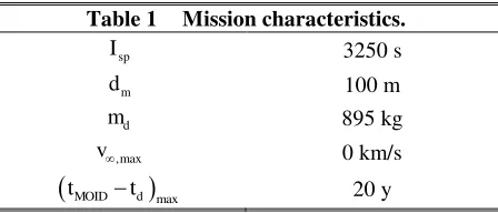
As a reference case, we consider a spacecraft equipped with a solar mirror with a diameter of 100 m and a dry mass md of 895 kg [29]. The spacecraft

is launched at a time td, selected in a range of 20

years before the possible collision, with zero velocity

at the sphere of influence of the Earth, and is equipped with engine delivering an unlimited thrust with a fix specific impulse of I_sp3250 s. Once the spacecraft has intercepted the asteroid, the slow-push deviation manoeuvre is performed from t_i up to the time at the MOID (i.e. tetMOID); no propellant is

assumed to be consumed during the deviation phase, but a 25% margin on the total wet mass is considered. Table 1 summarizes the key parameters of the mission.

Table 1 Mission characteristics. sp

I 3250 s

m

d 100 m

d

m 895 kg

,max

v_ 0 km/s



tMOIDtd



_max 20 y

The value of k was set according to the model of the solar collector developed in Ref. [30]. The value of k was chosen in order to obtain the same order of acceleration provided by a solar inflatable mirror, with a diameter d_m of 100÷110 m, along the range of distances from the Sun covered by the asteroid during its motion. Fig. 11 compares the acceleration computed through the full model described in Ref. [30], against Eq. (5), over a feasible range of distances for asteroid Apophis. Between the orbit apocentre and pericentre, Eq. (5) (represented with a solid line) gives an acceleration comparable with the one calculated through the full solar collector model (dash lines). Note that Eq. (5) does not take into account the decrease of the mass of the asteroid due to the ablation of the material, but this variation has been verified to be negligible in the domain of validity of the model.

0.7 0.75 0.8 0.85 0.9 0.95 1 1.05 1.1

0.6 0.8 1 1.2 1.4 1.6 1.8 2 2.2 2.4x 10

-11

r [AU]

at

[

km

/s

2]

a (dm=100 m)

a (dm=110m)

k/r2

Fig. 11 Magnitude of the acceleration for Apophis.

Final state equality constraints:

 Backward propagation: computation of the variation of Lagrange multipliers and variation of the control law

 Forward propagation of new control and trajectory

nominal control and trajectory:



u s_j, _j



Backward Recursion form tN1 to t1:  determination of *

j

u

 computation of the linear/quadratic expansion of the cost and return function is computed, about the point



*



,

j j

s u ;

 the coefficient _j is constructed and stored in memory

Forward Recursion form t to ₁ tN1:  computation of the new control and

trajectory



s uj, j



 step size adjustment procedure to obtain a new improved trajectory

convergence criterion

verify final

constraints end

yes yes

[image:11.612.321.545.209.305.2] [image:11.612.318.545.211.305.2] [image:11.612.335.518.544.686.2]

Table 2 reports the values of the acceleration constant k for asteroid Apophis, together with the average of the thrust acceleration on a nominal orbit of the asteroid, according to Eq. (5), the average of the Sun gravitational acceleration and the ratio between the two accelerations.

Table 2 Acceleration constant k and average of the accelerations acting on asteroid Apophis.

k [km3/s2] 2·105

Average thrust acceleration [km/s2] 1.09·10-11 Average gravitational acceleration

[km/s2] 6.8·10

-8

Acceleration ratio 1.6·10-4

A multi-objective optimisation was performed to minimise the vectorial objective function:







0



min m tw   r r  r  (14)

with respect to the launch date, the time of flight and the hyperbolic excess velocity. In Eq. (14) m0 is the

wet mass at the Earth defined as:





0 d p 1.25

m  m m  (15)

where m is the propellant mass for the transfer. p

w MOID d

t t t is the warning time and  r r is the total deviation to be maximized.

6.1.

Apophis Deviation Mission

[image:12.612.330.537.89.232.2]

In the following paragraph we report the results of a global search to identify candidate solutions for an interception and deviation mission to Apophis. A hypothetic impact is fixed on 15/05/2036 (13284 MJD since 2000). The results of the optimisation are represented in the set of Pareto optimal solutions in Fig. 12. The three axes report the components of the objective function in Eq. (14), respectively the initial mass m0, the warning time and the magnitude of the

deviation r . Note that, being the final mass at the asteroid interception fixed, the initial mass depends on of the propellant mass for the transfer leg. In the case of Apophis, a mission making use of a solar collector of 100 m achieves deviations of the order of 106 km, in a time range of 20 years, while solutions with 1000 days of warning time have a deviation of 13000 km.

1000 1500

2000 2500 3000

0 2000 4000 6000 80000

1 2 3 4 5

x 106

m₀ [kg] t

w [d]

||



r|

| [

k

m

]

Fig. 12 Pareto front for the deviation mission of Apophis.

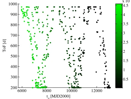
Fig. 13 represents the launch date and time of flight for the optimal solutions. The colour scale indicates the value of the corresponding achieved deviation.

6000 8000 10000 12000

200 300 400 500 600 700 800 900 1000

T

o

F

[

d

]

t_d [MJD2000]

0.5 1 1.5 2 2.5 3 3.5 4 4.5 x 106

Fig. 13 Launch window for the deviation mission of Apophis. The colour scale reports the value of the achieved deviation in km.

The modulus of the achieved deviation increases with the length of the thrust interval  t tMOIDti,

[image:12.612.64.299.165.237.2] [image:12.612.324.542.344.509.2]

0 1000 2000 3000 4000 5000 6000 70000 1 2 3 4 5 x 106

t [d]



-150 -100 -50 0 50 100 150

Fig. 14 Achieved deviation as a function of the push time. Asteroid Apophis. The colour scale indicates the angle at the interception of the asteroid in degrees.

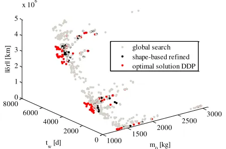
In order to verify the propellant mass estimation computed by means of the global search, 80 solutions of the 500 points of the Pareto set in Fig. 12 were locally optimised with the DDP method, according to the cost function in Eq. (10). The time constraints of each mission were fixed to the launch dates found through the global search (see Fig. 13). Therefore the locally optimised solutions have the same launch date and time of flight as the Pareto points, but a different thrust profile (i.e. the optimal thrust profile for the minimisation of the integral of the thrust square) and a different propellant mass. Fig. 15 highlights the point of the Pareto set which have been refined with the DDP algorithm. The black points belong to the original set of solutions and the red ones are the corresponding solutions after the local optimisation. Also in this case, Eq. (15) was used to compute the initial mass. In most of the cases the initial mass, required to achieve the same asteroid deviation, decreases with the refinement of the solution.

1000 1500

2000 2500 3000

0 2000 4000 6000 80000

1 2 3 4 5

x 106

m

0 [kg]

t_w [d]

||



r|

| [

k

m

] global search

[image:13.612.80.285.73.246.2]

shape-based refined optimal solution DDP

[image:13.612.328.553.82.230.2]

Fig. 15 Points of the Pareto front locally optimised through the DDP method.

Fig. 16 reports the percentage of propellant mass saved by the local optimisation of the trajectory, defined as:

, prelimiminary design , DDP optimised

, DDP optimised

100

p p

p

m m

m 



where mp, preliminary design is the propellant mass

estimated with the shape based method. In most of the cases the optimisation through the DDP method allows for a significant saving in propellant mass. However, some solutions present an increased propellant mass with respect to the preliminary design case; this is due to the different objective function used within the DDP algorithm. In fact the integral term of the cost function in Eq. (10) is equivalent to:

 2 1

d

d

t ToF

t

J T t dt





_

where T t  is the magnitude of the thrust vector

function of time. Instead the third term of the cost function in Eq. (14) indicates a minimisation of the propellant mass that, disregarding the constant coefficients, is:

 

1

d

d

t ToF

t

J T t dt





_

(16)

200 300 400 500 600 700 800 900 1000 -20

-10 0 10 20 30 40 50 60 70 80

ToF [d]

%

s

a

v

in

g

[image:14.612.328.537.77.246.2]

mp

Fig. 16 Percentage of propellant mass saved through the local optimisation of the solutions.

The preliminary design of the trajectory for the construction of the Pareto front did not include the transfer leg for escaping the Earth gravity field. In fact it was assumed the initial position of the spacecraft to be out of the sphere of influence of the Earth, with a zero relative velocity and a margin of 25% was added on the total wet mass.

In order to give an estimation of the propellant mass needed for the Earth escape, some trajectories were computed from an orbit around the Earth, by considering the Sun and the Earth as gravitational bodies. The optimisation was performed with the DDP algorithm; the trajectory was optimised as a whole, describing both the Earth centred and the Sun centred leg with respect to an inertial reference frame centred in the Earth. In this way it is possible to fully exploit the multi-body dynamics in the optimisation process.

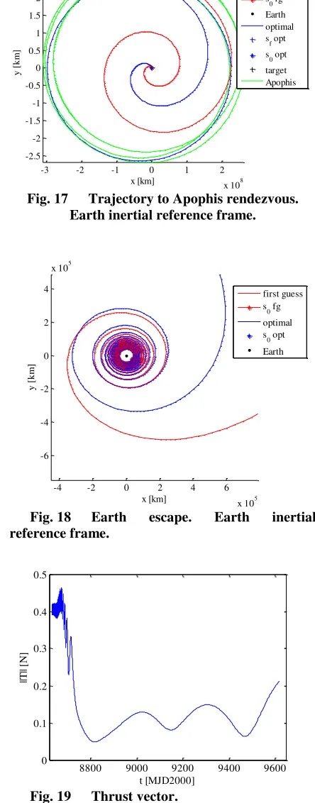
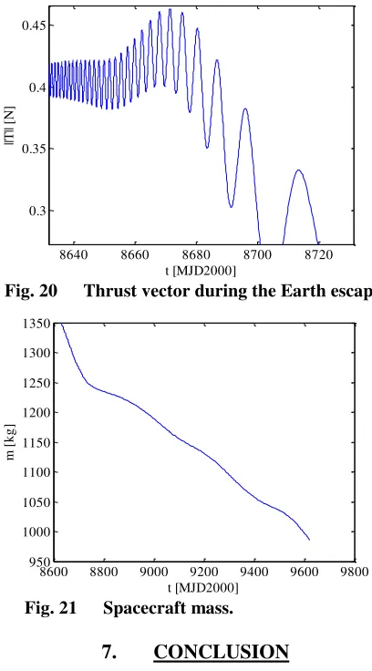
One of the trajectories optimised is presented in the following. An initial mass of 1350 kg was considered, with a specific impulse of 3250 s and no limits on the thrust magnitude. Fig. 17 shows the transfer trajectory in the Earth inertial reference frame. The red line represents the first guess and the blue line the optimal solution. The orbit of Apophis relative to the Earth is depicted with a green line. Fig. 18 presents a close up of the Earth escape leg, starting from a geostationary orbit. The magnitude of the thrust vector is reported in Fig. 19 and Fig. 20 and the mass of the spacecraft is shown in Fig. 21.

It has been computed that, for a mission with the these characteristics, the propellant mass needed to exit the sphere of influence of the Earth is about 100 kg and the time of flight of the transfer is increased of 100 days.

-3 -2 -1 0 1 2

x 108 -2.5

-2 -1.5 -1 -0.5 0 0.5 1 1.5 2 2.5

x 108

x [km]

y

[

k

m

]

first guess s

f fg s

0 fg Earth optimal s

f opt s

[image:14.612.78.284.79.243.2]

0 opt target Apophis

Fig. 17 Trajectory to Apophis rendezvous. Earth inertial reference frame.

-4 -2 0 2 4 6

x 105 -6

-4 -2 0 2 4

x 105

x [km]

y

[

k

m

]

first guess s

0 fg

optimal s

0 opt

[image:14.612.317.539.111.677.2]

Earth

Fig. 18 Earth escape. Earth inertial reference frame.

8800 9000 9200 9400 9600

0 0.1 0.2 0.3 0.4 0.5

t [MJD2000]

||T

||

[N

]

8640 8660 8680 8700 8720 0.3

0.35 0.4 0.45

t [MJD2000]

||T

||

[N

[image:15.612.73.277.81.449.2]

]

Fig. 20 Thrust vector during the Earth escape.

8600 8800 9000 9200 9400 9600 9800

950 1000 1050 1100 1150 1200 1250 1300 1350

t [MJD2000]

m

[

k

g

]

Fig. 21 Spacecraft mass.

7.

CONCLUSION

A solution to the asteroid deviation problem is proposed, which makes use of the proximal motion equations. Some semi-analytical formulae are used to calculate the total variation of the orbital elements when a low-push strategy is selected for the deflection phase. A global search was performed in the attempt of optimising the interception phase and the deviation phase as a whole. The preliminary design of the transfer trajectory was obtained through a shape based method and the solutions were refined by means of the differential dynamic programming method. In most of the cases a saving in propellant mass is saved through the local optimisation; this demonstrates that the design approach adopted within the global search is conservative. If the escape from the Earth gravity field is taken into account, the additional propellant mass can be accounted for in the 25% of mass margin. In this case an increase of the warning time has to be considered. As an application, a set of mitigation mission to Apophis was presented.

REFERENCES

[1] _“

Near-Earth Object Survey and Deflection Analysis of Alternatives”, NASA, 2007.

[2] _{Vasile M., “Ro}

bust Mission Design through Evidence

Theory and Multiagent Collaborative Search”, Annals of the New York Academy of Sciences, Vol. 1065, December 2005, pp. 152-173.

[3] _{Lawden D., “Rocket Trajectory Optimization: 1950}

-1963”, Journal of Guidance, Control and Dynamics, Vol. 14, No. 4, July-August 1991, pp. 705-711.

[4] _{Tsien H. S., “Take}

-off from Satellite Orbit”, Journal of the American Rocket Society, Vol. 23, July-August 1953, pp. 233-236.

[5] _{Benney D. J., “Escape from a Circular Orbit Using}

Tangential Thrust”, Jet Propulsion, Vol. 28, No. 3, March 1958, pp. 167-169.

[6] _{Boltz F., “Orbital Motion Under Continuous Radial}

Thrust”, Journal of Guidance, Control and Dynamics, Vol. 14, No. 3, May-June 1991, pp. 667-670.

[7] _{Boltz F., “Orbital Motion Under Continuous Tangential} Thrust”, Journal of Guidance, Control and Dynamics, Vol. 15, No. 6, 1992, pp. 1503-1507.

[8] _{Kechichian J. A., “Orbital Raising with Low} -Thrust

Tangential Acceleration in Presence of Earth Shadow”,

Journal of Spacecraft and Rockets, Vol. 24, No. 4, July-August 1998, pp. 516-525.

[9] _{Gao Y., Kluever C. A., “Analytic Orbital Averaging}

Technique for Computing Tangential-Thrust Trajectories”, Journal of Guidance, Control and Dynamics, Vol. 28, No. 6, November-December 2005, pp. 1320-1323.

[10] _{Petropoulos A. E., “Some Analytic}

Integrals of the Averaged Variational Equations for a Thrusting

Spacecraft”, Interplanetary Network Progress Report, Vol. 150, 2002, pp. 1-29.

[11] _{C. Colombo, M. Vasile, “Optimal Interception for NEO}

Deflection”, 58th International Astronautical Congress, Hyderabad, India, 2007. IAC-07-C1.4.02.

[12]

Schaub H., Junkins J. L., Analytical mechanics of space systems, AIAA Education Series, AIAA, 2003, pp. 592-623.

[13] _{Vasile M., Colombo C., “Optimal Impact Strategies fro}

Asteroid Deflection”, Journal of Guidance, Control and Dynamics, Vol. 31, No. 4, July-August 2008.

[14]

Battin R. H., An Introduction to the Mathematics and Methods of Astrodynamics, Revised Edition, AIAA Education Series, AIAA, 1999.

[15] _{Carusi A., Valsecchi G. B., D’abramo G., Bottini A.,}

“Deflecting NEOs in Route of Collision with the Earth”,

Icarus, Vol. 159, 2002, pp. 417-422.

[16] _{Scheeres D. J., Schweickart R. L., “The Mechanics of}

Moving Asteroids”, 2004 Planetary Conference: Protecting Earth from Asteroids, Orange Country, California, 23-26 February 2004.

[17]

Izzo D., “Optimization of Interplanetary Trajectories

for Impulsive and Continuous Asteroid Deflection” Journal of Guidance, Control and Dynamics, Vol. 30, No. 2, March-April 2007.

[19]

Jacobson D. H., Mayne D. Q., Differential Dynamic Programming, American Elsevier, New York, 1969. [20] _{Yakowitz S., “Theoretical and Computational}

Advances in Differential Dynamic Programming”, Control and Cybernetics, Vol. 17, No. 2-3, 1988, pp. 173-189. [21]

Yakowitz S., Rutherford B., “Computational Aspects of Discrete-Time Optimal Control”, Applied Mathematics and Computation, Vol. 15, 1984, pp. 29-45.

[22] _{Conway B. A., “Near}

-Optimal Defection of

Earth-Approaching Asteroids”, Journal of Guidance, Control and Dynamics, Vol. 24, No. 5, 2001, pp. 1035-1037.

[23]

Park S.-Y., Ross I. M., “Two-Body Optimization for Deflecting Earth-Crossing Asteroids”, Journal of Guidance, Control and Dynamics, Vol. 22, No. 3, 1999, pp. 995-1002.

[24] _{Kahle R., Hahn G., Kührt E., “Optimal Deflection of}

NEOs en route of collision with the Earth”, Icarus, Vol. 182, 2006, pp. 482-488.

[25] _{Carlson B.C., “Computing elliptic integrals by}

duplication”, Numerische Mathematik, Vol. 33, 1979, pp. 1-16.

[26] _{Vasile M., “A Behavioral}

-based Meta-heuristic for

Robust Global Trajectory Optimization”. IEEE, Congress on Evolutionary Computation, Singapore, 25-28 September 2007.

[27] _{Vasile M., De Pascale P., Casotto S., “On the}

Optimality of a Shape-based Approach on

Pseudo-Equinoctial Elements”, Acta Astronautica, Vol. 61, Reference Paper AA2820, 2007, pp. 286-297.

[28] _{Gershwin S. B., Jacobson D. H., “A Discrete} -Time Differential Dynamic Programming with Application to

Optimal Orbit Transfer”, AIAA Journal, Vol. 8, No. 9, 1970, pp. 1616-1626.

[29] _{Kahle R., Kuhrt E., Hahn G., Knollenberg J., “Physical}

limits of solar collectors in deflecting Earth-threatening

asteroids”, Aerospace Science and Technology, Vol. 10, 2006, pp. 256-263.

[30] _{Sanchez P., Colombo C., Vasile M., Radice G., “Multi} -criteria Comparison among Several Mitigation Strategies