Stochastic multiple mapping conditioning for a piloted, turbulent jet diffusion flame

      

City, University of London Institutional Repository

Citation

:

Vogiatzaki, K., Kronenburg, A., Navarro-Martinez, S. and Jones, W. P. (2011). Stochastic multiple mapping conditioning for a piloted, turbulent jet diffusion flame.

Proceedings of the Combustion Institute, 33(1), pp. 1523-1531. doi: 10.1016/j.proci.2010.06.126

This is the accepted version of the paper.

This version of the publication may differ from the final published

version.

Permanent repository link:

http://openaccess.city.ac.uk/8105/

Link to published version

:

http://dx.doi.org/10.1016/j.proci.2010.06.126

Copyright and reuse:

City Research Online aims to make research

outputs of City, University of London available to a wider audience.

Copyright and Moral Rights remain with the author(s) and/or copyright

holders. URLs from City Research Online may be freely distributed and

linked to.

City Research Online: http://openaccess.city.ac.uk/ [email protected]

Elsevier Editorial System(tm) for Proceedings of the Combustion Institute Manuscript Draft

Manuscript Number:

Title: Stochastic Multiple Mapping Conditioning for a turbulent jet diffusion flame

Article Type: Research Paper

Keywords: turbulent combustion modelling, turbulent diffusion flames, reacting flows, multiple mapping conditioning

Corresponding Author: Dr. Andreas Kronenburg,

Corresponding Author's Institution: University of Stuttgart

First Author: Konstantina Vogiatzaki

Order of Authors: Konstantina Vogiatzaki; Andreas Kronenburg; Salvador Navarro-Martinez; William P Jones

Abstract: A stochastic implementation of the Multiple Mapping Conditioning (MMC) approach has been applied to a turbulent jet diffusion flame (Sandia Flame D). This implementation combines the

advantages of the basic concepts of a mapping closure methodology with a probability density approach. A single reference variable has been chosen. Its evolution is described by a Markov process and then mapped to the mixture fraction space. Scalar micro-mixing is modelled by a modified ``interaction by exchange with the mean'' (IEM) mixing model where the particles mix with their -in reference space- conditionally averaged means. The formulation of the closure leads to localness of mixing in mixture fraction space and consequently improved localness in composition space. Results for mixture fraction and reactive species are in good agreement with the experimental data. The MMC methodology allows for the introduction of an additional ``minor dissipation time scale'' that controls the fluctuations around the conditional mean. A sensitivity analysis based on the conditional

Stochastic Multiple Mapping Conditioning for

a piloted, turbulent jet diffusion flame

K. Vogiatzaki

a

, A. Kronenburg

a,

∗

, S. Navarro-Martinez

b

,

W.P. Jones

b

a_{Institut f¨ur Technische Verbrennung, University of Stuttgart, 70569 Stuttgart,}

Germany

b_{Department of Mechanical Engineering, Imperial College London, SW7 2AZ,}

U.K.

Colloquium: Turbulent Flames

Total length is 5741 words determined by method 2 for latex users

main text: 3359; references: 402 (method 1)

Figure 1: 462 (two column figure)

Figure 2: 165

Figure 3: 165

Figure 4: 418 (two column figure)

Figure 5: 418 (two column figure)

Figure 6: 176

Figure 7: 176

∗ _{Corresponding author: A. Kronenburg, Institut f¨ur Technische Verbrennung,}

Uni-versity of Stuttgart, Herdweg 51, 70174 Stuttgart, Germany, Fax:+49-711-68555635

Email address: [email protected](A. Kronenburg).

Preprint submitted to Elsevier Science 5 January 2010

Stochastic Multiple Mapping Conditioning for

a piloted, turbulent jet diffusion flame

K. Vogiatzaki

a

, A. Kronenburg

a,

∗

, S. Navarro-Martinez

b

,

W.P. Jones

b

a_{Institut f¨ur Technische Verbrennung, University of Stuttgart, 70569 Stuttgart,}

Germany

b_{Department of Mechanical Engineering, Imperial College London, SW7 2AZ,}

U.K.

Colloquium: Turbulent Flames

Total length is 5741 words determined by method 2 for latex users

main text: 3359; references: 402 (method 1)

Figure 1: 462 (two column figure)

Figure 2: 165

Figure 3: 165

Figure 4: 418 (two column figure)

Figure 5: 418 (two column figure)

Figure 6: 176

Figure 7: 176

∗ _{Corresponding author: A. Kronenburg, Institut f¨ur Technische Verbrennung,} Uni-versity of Stuttgart, Herdweg 51, 70174 Stuttgart, Germany, Fax:+49-711-68555635

Email address: [email protected](A. Kronenburg).

Abstract

A stochastic implementation of the Multiple Mapping Conditioning (MMC)

ap-proach has been applied to a turbulent jet diffusion flame (Sandia Flame D). This

implementation combines the advantages of the basic concepts of a mapping closure

methodology with a probability density approach. A single reference variable has

been chosen. Its evolution is described by a Markov process and then mapped to the

mixture fraction space. Scalar micro-mixing is modelled by a modified “interaction

by exchange with the mean” (IEM) mixing model where the particles mix with their

-in reference space- conditionally averaged means. The formulation of the closure

leads to localness of mixing in mixture fraction space and consequently improved

localness in composition space. Results for mixture fraction and reactive species are

in good agreement with the experimental data. The MMC methodology allows for

the introduction of an additional “minor dissipation time scale” that controls the

fluctuations around the conditional mean. A sensitivity analysis based on the

con-ditional temperature fluctuations as a function of this time scale does not endorse

earlier estimates for its modelling, but only relatively large dissipation time scales of

the order of the integral turbulence time scale yield acceptable levels of conditional

fluctuations that agree with experiments. With the choice of a suitable dissipation

time scale, MMC-IEM thus provides a simple mixing model that is capable of

cap-turing extinction phenomena, and it gives improved predictions over conventional

PDF predictions using simple IEM mixing models.

Key words: turbulent diffusion flame, modelling, scalar mixing, multiple mapping

1 Introduction

As the concern for the environment increases and more stringent legislation

requires higher efficiency and reduced emissions, modern combustion systems

tend to use leaner mixtures and run at lower temperatures to restrict the

formation of _NOx. These facts lead to an increased interest in the modelling

of flows with substantial finite rate chemistry effects and advanced combustion

models that allow an accurate prediction of the interaction between chemical

reaction and turbulent mixing are needed.

Probabilistic methods such as the probability density function (PDF) [1]

meth-ods have been established as powerful modelling tools for combustion processes

since they allow for a direct and therefore, accurate closure of the chemical

reaction rate. However, the modelling of mixing process poses two problems:

Firstly, the lack of information on small scale structures and consequently lack

of information on the dissipation time and secondly, the requirement for the

mixing process of the stochastic particles to mimic the change in composition

of the real fluid particles due to turbulent mixing. These issues lead to certain

principles that should be satisfied by the mixing models such as boundedness

of the scalars, linearity of scalar transport, independence of the evolution of

the particle properties and -most importantly- localness in the physical and

compositional spaces. Detailed discussion regarding the importance of these

principles can be found in the the literature [1,2]. Here, we only emphasise

the importance of localness for mixing to occur [3]. Generally improvements

to the mixing model are limited by the resolution for the flow field and thus

discrepancies are more pronounced in the RANS context [4]. However, results

neighbour-hood in composition space so that mixing across the reaction zone is avoided,

the description of mixing is improved [2].

Different models have been suggested in the literature for the closure of the

mixing term. Simple models that are easy to implement such as the

“inter-action by exchange with the mean” (IEM) [5,6] and the various Curl’s

mod-els [7,8] do not ensure localness in composition space. In the present work,

we investigate the applicability of an approach that can ensure localness even

if mixing is based on a simple IEM models. Multiple mapping conditioning

(MMC) [9] combines the PDF method with the basic concepts of a mapping

closure for the modelling of the turbulent mixing term. MMC by itself does not

constitute a specific mixing model but it allows the modification of existing

models so that can accommodate the principles of localness while maintaining

their simplicity. The exact MMC model formulation used in the current work

is introduced in the following sections. The implementation methodology and

its limitations are described and predictions of the mixing field and of

reac-tive species are compared with experimental data for a piloted methane/air

jet diffusion flame (Sandia flame D) [10]. In addition, the sensitivity of the

method to an additional time scale, the minor dissipation time, is tested.

2 Reference space

The basic idea of the mapping closure concept [11,12] used in the MMC

methodology is to employ turbulent fluctuations and small-scale mixing in a

mathematical reference space,_ξ, with a known (or prescribed) PDF, to model

the turbulent fluctuations and small-scale mixing in the physical composition

leads to mapping functions that map the reference space to the physical space

and the conditional scalar dissipation appears in closed form [13,14]. In the

stochastic implementation the ”randomness” of species mass fraction _YI∗ of a

particle is assumed to be reflected by the randomness of the reference variable

ξ∗. This assumption generates three different definitions of fluctuations in the

MMC context: the unconditional fluctuations (_YI =_YI−_YI), the major

fluc-tuations (_Y =_YI|_ξ − _Y) and the minor fluctuations ((_YI =_YI− _YI|_ξ). In MMC, the particle position is tracked in reference space, mixing is allowed

only among particles that are close to each other in _ξ-space, and this directly

controls the minor fluctuations. Ideally, events that are close to each other in

physical space should also be close in composition space and thus in reference

space. If this is satisfied, localness of the MMC model is ensured.

One of the challenges of the method is the estimation of the “minor dissipation

time ”,_τmin, that controls the minor fluctuations. The minor fluctuations exist

only in the context of MMC, and the only indication for_τmin is that the level

of the minor fluctuations should lead to an accurate level of the “physical”

conditional fluctuations [15].

In a recent study by Clearyet al. [16], Sandia Flame D is modelled using one

reference variable obtained from a -to the particle position interpolated- LES

mixture fraction field. However, this approach cannot be applied to RANS.

Any particle properties interpolated from RANS statistics are mean properties

and do not add any information with respect to their instantaneous

compo-sitional localness. An alternative approached is described here that can be

considered an extention to the work of Wandel et al. [17]. It is a probabilistic

MMC formulation with a single reference variable that is used to enforce

process. MMC allows the choice of any number of reference variables, yet for

flames with low levels of local extinction, localness in mixture fraction space is

normally sufficient to indicate localness in the multidimensional composition

space.

We introduce the stochastic reference variable, _ξ∗, which is governed for one

single reference variable by the following set of stochastic differential equations

(sdes)

dx∗ =U(_ξ∗)_dt, (1)

dξ∗ =_Ao_dt+_bdw∗ (2)

and a Fokker-Planck equation

∂ρPξ

∂t +∇(UρPξ) +

∂AoρPξ

∂ξ −

∂2BρPξ

∂ξ2 = 0, (3)

where 2_B = _b2. If we assume a distribution for the reference space then the

drift and diffusion coefficients of Eq. (2) can be determined from Eq. (3).

3 The model

In the current implementation Eq. (1) and Eq. (2) that account for transport

in the physical and reference space respectively, are solved jointly with

that accounts for the evolution of the composition space. Ω_I is the reaction

rate and _SI∗ is the mixing term. A detailed derivation of Eqs.(1)-(4) can be

found in [9]

In this paper, one of the simplest models is examined for_SI∗: the IEM mixing

model. The original IEM model mixes all particles within one computational

cell with their unconditional means and conventional PDF computations with

IEM are denoted from hereon PDF-IEM. When using the modified IEM model

(MMC-IEM) the particles are mixed with their means conditioned on a certain

value in reference space, _YI |_ξ.

According to the MMC-IEM model, _SI∗ is then given by

SI∗ =

YI(ξ∗)−YI∗

τmin ,

(5)

with _{< S}∗|_ξ∗ =_{ξ, x}∗ =_{x >}= 0 [9].

The simplicity of the IEM model is attractive for implementation, especially as

a first modelling attempt that is expected to provide qualitative

understand-ing of the stochastic implementation of the MMC method and its application

to real flames. However, a good estimate of the minor dissipation time needs

to be determined. As Pope [18] pointed out PDF predictions are sensitive to

the velocity-to-scalar time scale ratio _CYa value that is not known a priory.

Klimenko [15] suggested that the minor dissipation time should be

consider-ably smaller than the characteristic physical dissipation time, _τD, performing

an asymptotic analysis for an homogeneous case, and Direct Numerical

Sim-ulations (DNS) for simple homogeneous flows indeed suggest_τmin ≈1_/8_τD as

flames DNS is not an option, and it is far from being clear how to extract

the correct dissipation time from RANS solutions for the flow field. Here, we

report on results using three different values for_τmin.

For the current implementation a single “mixture fraction-like” reference

vari-able is used. The term mixture-fraction like varivari-able has the connotation that

closeness in reference space guarantees closeness in mixture fraction space. For

the derivation of coefficients_Ao _{andB a Gaussian distribution ofξ}∗_{is assumed,}

and the coefficients are then given in the following form [9]

U=U(_ξ;x_{, t}) =U(0)+U(1)_ξ, (6)

Ao =−∂B

∂ξ +Bξ+

1

ρ∇ρU

(1)₊ 2

Pξ

∂BPξ

∂ξ , (7)

U(0) =v_, (8)

U(1)ξZ=vZ, (9)

wherev is the mean flow field velocity. The turbulent flux can be modelled by

a standard gradient approximation (v_Z = −_D∇ _{< Z >}). _B is modelled

independently of_ξ, (_B =_B(x_{, t})) [9], and is related to scalar dissipation_NZ

by

B

∂Z ∂ξ

₂

=_NZ. (10)

In addition, the derivative _∂Z/∂ξ is approximated by _∂Z/∂ξ.

It is apparent from Eq. (10) that closure of the MMC model requires

knowl-edge of the unconditional scalar dissipation of_Z. The parameter_NZ can be

modelled adopting Corrsin’s suggestion [19] that the decay rate of a passive

kinetic energy i.e.

NZ= Z

₂

τD ,

(11)

where _τD is proportional to the flow turbulent time scale _τ = _k/ε with

pro-portionality constant commonly assumed to be _CD = 1.

It might appear as a paradox that a distribution is assumed for a variable that

in reality is solved. Equation (2), however, is solved such that every particle

has its own stochastic value of_ξ∗ that is indicative of the distance of -say- two

particles in mixture fraction space. Attributing a random value for_ξ∗ to every

particle that is derived from a Gaussian distribution, without solving Eq. (2)

might present itself as an alternative that would maintain the Gaussianity of

the reference space, however, it would not offer any extra information with

respect to the distance of particles in mixture fraction space. Instead, using

the specific model for _Ao and _B introduces links between the physical space

and the reference space through_U(_ξ), _NZ and _Zξ.

4 Test case and numerical implementation

The test case (Sandia Flame D) [20,10] consists of a methane/air fuel mixture

that issues from a central 7.2mm diameter nozzle surrounded by coaxial pilot

flame with an outer diameter of 18.2mm. The fuel is 25% _CH4 and 75% air

by volume with a stoichiometric mixture fraction of _Zst = 0_.351. The jet

Reynolds number is 22,400, the pilot inlet velocity is 11_m/s and the velocity

of the co-flowing air is 0_.9_m/s.

(BOFFIN). Turbulence is modeled by a standard _k-_ε model. A cylindrical

domain extends 0_.65_m in downstream direction and 0_.15_m in radial direction

and is discretised by 80 axial and 50 radial finite volume cells. For the

compo-sition field there are 800.000 Lagrangian particles corresponding to an average

number of around 200 particles per cell. The evolution of the particle

prop-erties is modelled by Eqs. (1), (2) and (4). It is important to emphasise that

every particle carries information on its (stochastic) velocity, species

concen-tration and_ξ. Note that the reference space is Gaussian and unbounded, but

the determinisic drift term counteracts the random diffusion term and keeps

particles close to the mean. Then, depending on their _ξ value, the particles

within each cell are ordered in the reference sample space that extends from

-4 to 4 and that is divided into 40 bins. Chemistry is modelled by a reduced

15-step methane-air mechanisms [21].

Two extra equations for the mean mixture fraction and its variance are also

solved in the RANS context. Conventional closure are used for these

deter-ministic equations for_Z and _Z2. The values are used to initialise_Z∗ and

for comparison with the stochastic solutions for the mixing field.

The mapping functions of mixture fraction and of the reactive species _YI(_ξ∗)

are obtained from a binning procedure. In every Eulerian cell the sample space

of the reference variable is defined and divided into a number of bins. Then

the particles that are in the cell are ordered depending their_ξ∗ value. In each

ξ-bin, _YI(_ξ) is defined by an ordinary averaging process. For the _ξ-bins that

are empty, values are obtained from linear interpolation. The computation

of _YI(_ξ) is needed for the mixing with the conditional mean, postulated by

5 Results

Three computations with different minor dissipation times have been run and

are compared with experiments and solutions from deterministic,

Reynolds-averaged transport equations for mean mixture fraction and its variance. The

three mixing time scales that are investigated here are_τmin =_τd,_τmin = 0_.7_τd

and _τmin = 0_.5_τd.

Figure 1 shows the mixture fraction profiles over the reference space at various

axial locations and_r/D = 1 for the three test cases of the MMC-IEM mixing

model. It can be seen that particles cluster around the conditional mean (solid

line). At upstream locations the slope is rather moderate due to the low

mix-ture fraction variance in these areas. Downstream the slope increases. There is

significant scatter around_Z(_ξ) for all three cases, however there are

quantita-tive differences. As_τmin decreases, mixing becomes more intense, particles are

mixed faster towards their conditional means and fluctuations are reduced.

This - of course- affects predictions for mixture fraction mean and in particular

its variance. Figures 2 and 3 show radial profiles of mean and rms of mixture

fraction _Z at different axial locations. Predictions MMC-IEM are presented

and compared with experimental data. Predictions from the solution of the

conventional RANS equations (solid lines) and from PDF-IEM (diamonds) are

also included, but no results are shown for_τmin = 0_.7_τd for clarity of

presen-tation. Predicted mixture fractions and rms generally fall between predicted

values for _τmin =_τd and _τmin = 0_.5_τd.

Overall the predictions are in qualitative agreement with the experimental

in the domain and the differences are rather small between all models. With

respect to mixture fraction variance, differences are more pronounced. The

predictions are generally good and they constitute a slight improvement in

comparison to the deterministic RANS and PDF-IEM predictions. However,

the effects of different time scales are apparent and consistent with Fig.1.

In Fig.3, dashed lines denote computations with _τmin = _τD and stars

repre-sent _τmin = 0_.5_τD. A smaller mixing time scale enhances mixing, it reduces

the scatter around the conditional mean and therefore, predicted _Z2 are

noticeably decreased.

It is noted that MMC-IEM profiles are not smooth which can be attributed to

the stochastic MMC implementation. The derivation of the drift and diffusion

coefficients of Eq. (3) is based on the assumption of a normal distribution for

ξ∗. It is important for the accuracy of the method that the computed PDFs

remain close to the presumed distribution throughout the simulation. For all

three test cases the agreement with the normal distribution is satisfactory

(not shown), but 200 particles per cell do certainly not reproduce the exact

continuous Gaussian distribution. Further, computation of _YI∗|_ξ∗ =_ξ

intro-duces inaccuracies. The conditional mean _YI∗|_ξ∗ =_ξ is calculated for every

ξ bin and therefore the calculation is based on a considerably smaller number

of particles than present in the corresponding RANS cell. Temporal averaging

may alleviate these problems but this is not attempted here.

The mixing model performance is now evaluated in terms of scatter plots of

mixture fraction and reactive species. This is presented in Figs 4 and 5 for

the MMC-IEM model. The column to the left shows the experimental data,

the three columns in the middle show MMC-IEM for the three different time

computa-tions. The agreement with experimental data in terms of conditional species

profiles and peak values is rather satisfying. The degree of scattering around

stoichiometric, however, is somewhat underpredicted for all time scales and

our model does not seem to predict local extinction that is evident in the

experiments very accurately. However, the effects of _τmin are evident. Only

a minimum dissipation time scale of the order of the integral turbulent time

scale allows some deviation from a fully burning flamelet regimes. Stronger

mixing in conditional (reference) space inhibits all significant deviations from

the conditional mean and reduces the degree of extinction. Small time scales

of the order of 0_.1_τD as suggested by [15,17], would significantly overpredict

conditional mixing in Sandia Flame D, and MMC-IEM would yield very smilar

prediction as PDF-IEM where conditional mixing is not explicitly modelled.

It can be seen in the right column that PDF-IEM predictions do not exhibit

much scatter around the conditional mean which is consistent with results

reported in the literature[4]. MMC-IEM is thus distincly different from

PDF-IEM that tends to destroy all conditional fluctuations, but a suitable estimate

of _τmin should be larger than _τmin = 0_.5_τD. Estimates of _τmin ∈ 0_.7_τD,1_.0_τD

seem consistent with experiments. An increase of the minimum dissipation

time scale above _τmin = _τD does not seem physical and cannot be justified.

Not surprisingly, additional computations (results not shown here) have given

a considerable overprediction of the mixture fraction fluctuations that cannot

be consolidated with the experimental data.

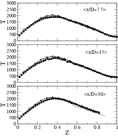
A better quantitative estimate is given in Figs 6 and 7 where temperatures

and their RMS are conditionally averaged on mixture fraction and plotted for

different downstream positions. MMC-IEM and PDF-IEM give good

predic-tions for the conditional temperatures. They are slightly overpredicted due

and 5. Small differences can be seen for the conditional mean at _x/D = 15

where MMC-IEM with _τmin =_τD gives somewhat lower temperature

predic-tion due to the decreased mixing, the increased scatter and therefore increase

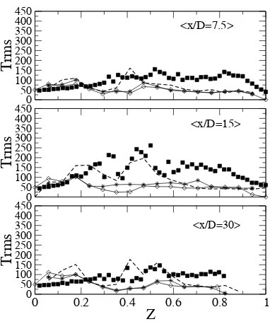
local extinction. Differences are more pronounced in Fig.7. It is apparent that

PDF-IEM and MMC-IEM with a small minimum dissipation time scale does

not allow for the correct level of conditional fluctuations and the mixing

implic-itly oppresses variations in conditional temperature. Longer time scales yield a

relatively accurate level of conditional fluctuations, in particular at_x/D = 15

and possibly _x/D = 30. It is not yet quite clear why conditional fluctuations

remain relatively low at_x/D = 7_.5, but improvements to conventional mixing

models are clear.

6 Conclusion

The current work is one of the first implementions of stochastic MMC coupled

to a RANS solver for the computation of mixing and reaction in a turbulent

jet flame. A single Markovian reference variable with Gaussian distribution

is selected and mapped to the mixture fraction space. The advantage of the

method is that despite the use of a very simple mixing model such as IEM, the

localness in composition space can be enforced and the conditional fluctuations

can be modelled more accurately and be better controlled. MMC can capture

parts of the physical behaviour of moderately complex phenomena such as

extinction and ignition and can provide accurate levels of fluctuations if a

suitable estimate of _τmin is found. It has been shown that for a turbulent jet

flame such as Sandia Flame D, the appropriate time scale needs to be close

to the integral turbulence time scale and good predictions of all quantities of

scalars and their fluctuations can be achieved. Further studies, however, would

need to establish the dependence of _τmin on Reynolds number and/or flow

geometries.

7 Acknowledgments

The authors would like to thank Dr M.J. Cleary for many helpful discussions.

SNM acknowledges the financial support by The Royal Society.

References

[1] S. Pope, Prog. Energy Combust. Sci.11 (2) (1985) 119 – 192.

[2] S. Subramaniam, S. Pope,Combust. Flame 115 (4) (1998) 487–514.

[3] A. Norris, S. Pope,Combust. Flame 83 (1-2) (1991) 27–42.

[4] S. Mitarai, J. Riley, G. Kosly,Phys. Fluids17 (4) (2005) 047101 – 1–047101–15.

[5] C. Dopazo, Phys. Fluids 22 (1) (1979) 20–39.

[6] E. O’Brien,Turbulent Reacting Flows, Springer-Verlang, 1980.

[7] R. Curl,AIChE Journal 9 (1963) 175–181.

[8] J. Janicka, W. Kolbe, W. Kollmann, J. Non-Equilib. Thermodyn. 4 (1) (1979)

47 – 66.

[9] A. Klimenko, S. Pope,Phys. Fluids 15 (7) (2003) 1907–1925.

[10] R. Barlow, J. Frank,Piloted methane/air flames C, D, E, and F - Release 2.0,

Tech. rep., Sandia National Laboratories (2003).

[12] S. Pope, Theor. Comput. Fluid Dyn.2 (5-6) (1991) 255–270.

[13] A. Kronenburg, M. Cleary, Combust. Flame 155 (1-2) (2008) 215–231.

[14] K. Vogiatzaki, M. Cleary, A. Kronenburg, J. Kent, Phys. Fluids 21 (2).

[15] A. Klimenko,Combust. Flame 143 (4) (2005) 369–385.

[16] M. Cleary, A. Klimenko, Flow Turb. Comb. 82 (4) (2008) 477–491.

[17] A. Wandel, A. Klimenko,Phys. Fluids 17 (12).

[18] S. Pope, Proceedings of the Sixth International Workshop on Turbulent

Non-Premixed Flames.

[19] S. Corrsin,J. Aeronaut. Sci.18 (1951) 417.

[20] R. Barlow, J. Frank, A. Karpetis, J.-Y. Chen, Combustion and Flame 143 (4)

(2005) 433 – 449.

8 Figures 0 0.2 0.4 0.6 0.8 1 0 0.2 0.4 0.6 0.8 1 Z( 

-4 -2 0 2 4

 0 0.2 0.4 0.6 0.8 1

-4 -2 0 2 4

 -4 -2 0 2 4

<x/D=3> <x/D=3> <x/D=15> <x/D=30> <x/D=3> <x/D=15> <x/D=30> <x/D=15> <x/D=30>

Fig. 1. Profiles of the mixture fraction in reference space at various axial locations and r/D= 1 for τ_min =τ_d (top row), τ_min = 0.7τ_d (middle row) andτ_min = 0.5τ_d (bottom row). Solid lines are the profiles ofZ(ξ) and symbols represent the particles.

0 0.2 0.4 0.6 0.8 1 0 0.2 0.4 0.6 0.8 1

Z [ - ]

0 1 2 3 4 5 6 r/D [ - ] 0 0.2 0.4 0.6 0.8 1

0 1 2 3 4 5 6 r/D [ - ] <x/D=01>

~

<x/D=03>

<x/D=7.5> <x/D=15>

[image:20.612.134.446.55.301.2]

<x/D=30> <x/D=45>

[image:20.612.199.384.435.594.2]

0 0.1 0.2 0.3 0.4 0 0.1 0.2 0.3 0.4

Zrms [ - ]

0 1 2 3 4 5 6 r/D [ - ] 0

0.1 0.2 0.3 0.4

0 1 2 3 4 5 6 r/D [ - ] <x/D=01> <x/D=03>

<x/D=7.5> <x/D=15>

[image:21.612.196.384.59.216.2]

<x/D=30> <x/D=45>

Fig. 3. Radial profiles of mixture fraction rms at different axial locations. Squares represent the experimental data, solid lines the predictions from conventional RANS equations, dashed lines the predictions from the MMC-IEM mixing model with τ_min = τ_D, stars the predictions from the MMC-IEM mixing model with τmin = 0.5τD and diamonds the predictions from PDF-IEM.

500 1000 1500 2000 2500

T [ K ]

0.04 0.08 0.12 0.16

CH

4

0 0.2 0.4 0.6 0.8 1 Z 0 0.04 0.08 0.12 0.16

CO

0.2 0.4 0.6 0.8 1

Z 0.2 0.4 0.6 0.8 1Z 0.2 0.4 0.6 0.8 1Z 0.2 0.4 0.6 0.8 1Z

_D

_D

0.7_D 0.5_D

Exp.

_D Exp.

Exp.

0.7_D

0.7_D

0.5_D

0.5_D

IEM

IEM

IEM

[image:21.612.95.488.378.610.2]

500 1000 1500 2000 2500

T [ K ]

0.04 0.08 0.12 0.16

CH

4

0 0.2 0.4 0.6 0.8 1 Z 0 0.04 0.08 0.12 0.16

CO

0.2 0.4 0.6 0.8 1

Z 0.2 0.4 0.6 0.8 1Z 0.2 0.4 0.6 0.8 1Z 0.2 0.4 0.6 0.8 1Z

_D

_D

0.7_D 0.5_D

Exp.

_D Exp.

Exp.

0.5_D

0.7_D

0.5_D

0.5_D

IEM

IEM

[image:22.612.93.488.50.279.2]

IEM

Fig. 5. Scatter plots of T, CH₄ and CO as functions of mixture fraction atx/D = 30.

0 500 1000 1500 2000 2500 3000 T 0 500 1000 1500 2000 2500 3000 T

0 0.2 0.4 0.6 0.8 1

Z 0 500 1000 1500 2000 2500 3000 T <x/D=7.5> <x/D=15> <x/D=30>

[image:22.612.194.384.361.581.2]

0 50 100 150 200 250 300 350 400 450

Trms

0 50 100 150 200 250 300 350 400 450

Trms

0 0.2 0.4 0.6 0.8 1

Z

0 50 100 150 200 250 300 350 400 450

Trms

<x/D=7.5>

<x/D=15>

[image:23.612.194.385.193.422.2]

<x/D=30>

List of Figures

1 Profiles of the mixture fraction in reference space at various

axial locations and _r/D = 1 for _τmin = _τd (top row),

τmin = 0.7τd (middle row) and τmin = 0.5τd (bottom row).

Solid lines are the profiles of _Z(_ξ) and symbols represent the

particles. 17

2 Radial profiles of mean mixture fraction at different axial

locations. Squares represent the experimental data, solid lines

the predictions from conventional RANS equations, dashed

lines the predictions from the MMC-IEM mixing model with

τmin =τD, stars the predictions from the MMC-IEM mixing

model with _τmin = 0_.5_τD and diamonds the predictions from

PDF-IEM. 17

3 Radial profiles of mixture fraction rms at different axial

locations. Squares represent the experimental data, solid lines

the predictions from conventional RANS equations, dashed

lines the predictions from the MMC-IEM mixing model with

τmin =τD, stars the predictions from the MMC-IEM mixing

model with _τmin = 0_.5_τD and diamonds the predictions from

PDF-IEM. 18

4 Scatter plots of T, CH₄ and CO as functions of mixture

fraction at_x/D = 15. 18

5 Scatter plots of T, CH₄ and CO as functions of mixture

6 Conditionally averaged temperature at different axial

locations. Squares represent the experimental data, dashed

lines the predictions from the MMC-IEM mixing model with

τmin =τD, stars the predictions from the MMC-IEM mixing

model with _τmin = 0_.5_τD and diamonds the predictions from

the PDF-IEM simulations. 19

7 Conditionally averaged temperature RMS at different axial

locations. Squares represent the experimental data, dashed

lines the predictions from the MMC-IEM mixing model with

τmin =τD, stars the predictions from the MMC-IEM mixing

model with _τmin = 0_.5_τD and diamonds the predictions from