Quantifying and minimising systematic and random errors in X-ray micro-tomography based volume measurements

(1)

Quantifying and minimising systematic and random errors in X-ray

micro-tomography based volume measurements

Q. Lin

a

, S.J. Neethling

a,n

, K.J. Dobson

b,c

, L. Courtois

b,c

, P.D. Lee

b,c a

Rio Tinto Centre for Advanced Mineral Recovery, Department of Earth Science and Engineering, Imperial College London, London SW7 2AZ, UK b_{Manchester X-ray Imaging Facility, School of Materials, University of Manchester, Oxford Rd., Manchester M13 9PL, UK}

c

Research Complex at Harwell, Rutherford Appleton Laboratories, Harwell, Didcot, Oxfordshire, OX11 0FA, UK

a r t i c l e i n f o

Article history: Received 23 July 2014 Received in revised form 13 November 2014 Accepted 31 December 2014 Available online 1 January 2015

Keywords: Micro-CT Grain tracking Uncertainty Error propagation

a b s t r a c t

X-ray micro-tomography (XMT) is increasingly used for the quantitative analysis of the volumes of features within the 3D images. As with any measurement, there will be error and uncertainty associated with these measurements. In this paper a method for quantifying both the systematic and random components of this error in the measured volume is presented. The systematic error is the offset between the actual and measured volume which is consistent between different measurements and can therefore be eliminated by appropriate calibration. In XMT measurements this is often caused by an inappropriate threshold value. The random error is not associated with any systematic offset in the measured volume and could be caused, for instance, by variations in the location of the speciﬁc object relative to the voxel grid. It can be eliminated by repeated measurements. It was found that both the systematic and random components of the error are a strong function of the size of the object measured relative to the voxel size. The relative error in the volume was found to follow approximately a power law relationship with the volume of the object, but with an exponent that implied, unexpectedly, that the relative error was proportional to the radius of the object for small objects, though the exponent did imply that the relative error was approximately proportional to the surface area of the object for larger objects. In an example application involving the size of mineral grains in an ore sample, the uncertainty associated with the random error in the volume is larger than the object itself for objects smaller than about 8 voxels and is greater than 10% for any object smaller than about 260 voxels. A methodology is presented for reducing the random error by combining the results from either multiple scans of the same object or scans of multiple similar objects, with an uncertainty of less than 5% requiring 12 objects of 100 voxels or 600 objects of 4 voxels. As the systematic error in a measurement cannot be eliminated by combining the results from multiple measurements, this paper introduces a procedure for using volume standards to reduce the systematic error, especially for smaller objects where the relative error is larger.

&2015 The Authors. Published by Elsevier Ltd. This is an open access article under the CC BY license (http://creativecommons.org/licenses/by/4.0/).

1. Introduction

X-ray micro-tomography (XMT) is a popular technique for the non-destructive qualitative and quantitative investigation of the internal structure of objects. It has been widely applied across material science (Puncreobutr et al., 2012; Stock, 1999), en-gineering (Aydoğan et al., 2006;Ghorbani et al., 2011;Ketcham and Carlson, 2001) and biological sciences (Yue et al., 2011) to provide quantitative data about the structure and morphology of 3D objects and features within them (crystals, pores, fractures etc.).

For the measurement of object or feature volumes from XMT images, each voxel (smallest volume element, equivalent to a 3D pixel) belonging to a feature or object is obtained using a thresholding algorithm, and the volume obtained by counting the relevant voxels. However, the boundaries of features rarely coin-cide with the boundaries of the regular voxel grid, leading to the

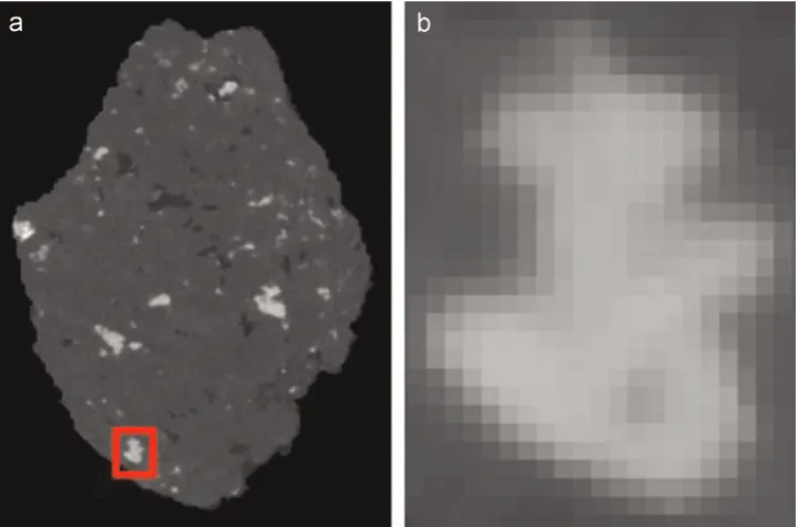
“partial volume effect”at the interface, where voxels have an in-termediate bulk composition, and there is some uncertainty in the exact boundary location (Ketcham and Carlson, 2001;Stock, 1999). Theoretically the partial volume effect should only affect a narrow (few voxel) region when the boundary is planar, smooth and sharp, but in certain systems boundaries can be uneven and dif-fuse (Fig. 1).

The choice of thresholding algorithm or threshold value will have a systematic effect on the measured volume, while variability in the exact location of the object relative to the voxel grid will Contents lists available atScienceDirect

journal homepage:www.elsevier.com/locate/cageo

Computers & Geosciences

http://dx.doi.org/10.1016/j.cageo.2014.12.008

0098-3004/&2015 The Authors. Published by Elsevier Ltd. This is an open access article under the CC BY license (http://creativecommons.org/licenses/by/4.0/). n_{Correspondence to: Department of Earth Science and Engineering, Royal School}

of Mines, Imperial College London, London SW7 2BP, UK. E-mail address:[email protected](S.J. Neethling).

(2)

cause a random variation in the measured volume. The relative impact on the measured volume of both these systematic and random errors will be strongly dependent on the size of the object relative to the voxel size, as the proportion of the volume that is within the uncertain region at the boundaries of objects will de-crease as the object size inde-creases.

In this paper we describe a procedure for quantifying both the systematic and random components of this uncertainty in volume. In particular, we describe how to ascertain how many times an object needs to be scanned (or how many similar objects in the same scan need to be combined) to achieve a given level of ac-curacy in the measured volume, assuming that any systematic error has been eliminated. Repeatability will also be inﬂuenced by both the random and systematic components of the error as the systematic error is likely to change from scan to scan, while the random component will add uncertainty to the measurement. Although the methodology presented signiﬁcantly improved re-peatability, for absolute dimensional accuracy calibration with an appropriate phantom is required.

While our methodology is applicable to a wide range of 3D image analysis applications, the results obtained will depend to some degree on the sample being studied and the specifics of the scanner used. In this paper the example used is the quantification of metal sulphide grain volumes within an ore particle/rock frag-ment. The ore particles were scanned using a Nikon Metris 225 XYTH Custom Bay with a 1 mm aluminium filter to reduce the effect of beam hardening, 89 kV energy, 0.708 s exposure time and 2001 projections. The detector size was 20002000 pixels, giving a linear resolution of approximately 17

μ

m for the magniﬁcation selected. We chose this example as there are a large number of mineral grains within the image volume and these grains are known to have a wide volume distribution. For the scan resolution used the mineral grains range from sub-voxel sizes to tens of thousands of voxels, allowing for the effect of the volume of the object to be studied over many orders of magnitude.

A key requirement of this methodology is the ability to identify the same objects in repeated scans. An algorithm developed for tracking the dissolution of mineral grains as they undergo leaching is used for this purpose. Theﬁrst section of this paper thus gives a

short description of this algorithm as the data generated from it is the source of the statistical analysis.

2. Grain tracking and identiﬁcation methodology

The procedure for the image processing was:

1. A 333 median_ﬁlter was applied to reduce the noise level. 2. The transformation matrix to align subsequent scans to the orientation and location of the reference scan was calculated and extracted (Studholme et al., 1999).

3. The threshold for distinguishing the ore particles from the air phase was obtained using the Otsu algorithm (Otsu, 1979), while the metal sulphide grains are distinguished from the ore matrix using a maximum entropy algorithm (Kapur et al., 1985). The reason for the different algorithms is that the air and rock have very distinct peaks in the intensity histogram, while the relatively small volume of metal sulphide present means that there is no distinct peak in the histogram.

4. The individual grains were then tracked across different images.

The algorithm starts by identifying all the mineral grains of interest in the reference image. The connectivity of the grains are analysed so that each isolated grain is given a unique identifier. On subsequent images voxels that are identified as mineral grains need to be given the same identifier number as they had in the original image. This is achieved by using a mask based on the reference image. This mask is rotated and translated to match the location and orientation of the ore particle in the subsequent image. This mask is then applied to the mineral grains.

[image:2.595.113.474.58.296.2]

Since the grains do not grow between images, this masking would be all that is required if the thresholding of the images and the translation and rotation of the mask were perfect. In general this is not the case and unassigned rims can remain around the masked grains. This problem is resolved by assigning these rim voxels the identi_fier of a neighbouring identi_fied voxel. This pro-cess is repeated until all voxels in the intensity range are identified

Fig. 1.(a) A 2D slice through a 3D tomography volume of example data showing mineral grains within an ore particle. (b) A region of interest demonstrating diffuse

boundaries.

(3)

or discarded.

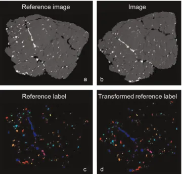
It should be noted that in this algorithm it is the mask that is rotated and translated and not the data itself. Rotating the data would have an effect on the measured volume of the grains and thus also the error associated with the volume measurement as the interpolation required to project the rotated and translated data back onto a grid will cause the boundaries to become even more diffuse. Translating and rotating the mask will cause slight changes in the size and shape of masked regions, but this will have virtually no impact on the algorithm as the rims that result from slight errors in the mask are accounted for in the algorithm.Fig. 2 shows an example of a reference and subsequent image as well as the original and transformed mask. Note that, while the ﬁgure shows a 2D slice, the rotations and translations were all 3D.

This identi_ﬁcation method has a few assumptions and limita-tions. Firstly, any objects that do not appear in the initial image but exist in a later scan are not counted. This issue can occur for ob-jects that are of a size very close to the voxel resolution or due to phantom particles caused by noise in the image, which can be ameliorated by the use of a medianﬁlter. Another potential issue with this algorithm is if the mask does not overlap any portion of the object in subsequent images. Again this is only likely for ob-jects that are approximately the same size as the voxel resolution. Objects that appear in the reference scan, but are not observed in the subsequent scan are included in the statistics, though objects that are not in the reference scan, but appear in a subsequent scan are not counted. These objects make up about 5% of the total number of objects in the subsequent scan, but as their sizes are all close to the scan resolution they account for only 0.05% of the total

volume of the identiﬁed objects.

3. Error and uncertainty in the volume of scanned objects

Before the volume data can be used with conﬁdence the sys-tematic and random errors in the measurement need to be un-derstood. Systematic errors are those in which the error is the same for all similar objects and, for volume measurement, will typically be a function of the size of that object. Correction of systematic errors is possible using appropriate standards and ca-libration. Random errors are those that are not the same for si-milar objects or between scans and thus add an uncertainty to measurements that cannot be eliminated by calibration. However, unlike systematic errors, random errors do not in_ﬂuence the average measured volume if enough volume measurements have been used. What this paper will demonstrate is a methodology for determining how many repeat measurements (or measurements of similar objects) need to be made to reduce the uncertainty caused by the random error to an appropriately small value (what is considered appropriately small will, of course, depend upon the application).

[image:3.595.123.484.57.401.2]

The systematic error in the grain volume will come about from effects such as an error in the threshold used, while the random error will come about due to effects such as the change in the partial volume effect due to the speciﬁc location of the mineral grain relative to the voxel grid, which will change from scan to scan and from grain to grain.

Fig. 2.Example of reference label transformation. (a) Reference image. (b) Image in subsequence scan. (c) Label mask for reference image. (d) Transformed reference label

after applying 44 transformation matrix. The transformation matrix is calculated using (a) and (b).

(4)

3.1. Sensitivity of measured volume to threshold changes

Global thresholding is a common method to distinguish dif-ferent phases (Gonzalez et al., 2003), and the choice of threshold used to distinguish the phases can have a large effect on the vo-lume measured. Thresholding is an important step in the image quanti_ﬁcation and it has a direct relationship with the uncertainty, especially for smaller grains. Much of this uncertainty arises from partial volume effect, where the edges of grains are blurred due to the fact that they do not necessarily align with the voxels. Typi-cally an algorithm is used to choose the threshold to reduce sub-jectivity in the identiﬁcation of the objects within the image, but this does not mean that systematic errors due to thresholding are eliminated and it might well be appropriate to adjust the thresh-old value to minimise these systematic errors if an accurate, rather than simply consistent, volume measurement is required.

Local thresholding algorithms can also be used (Gonzalez et al., 2003). While the trends in random error associated with local algorithms are likely to be similar to those associated with global methods, as these errors are largely associated with the real un-certainty in the images, the systematic errors will be very algo-rithm speciﬁc. For this reason this paper concentrates on the un-certainties and errors associated with global thresholding as these responses are the same irrespective of which algorithm is used to choose the threshold (the response in the measured volume brought about by varying the threshold value will be the same irrespective of the algorithm used to obtain the initial threshold value).

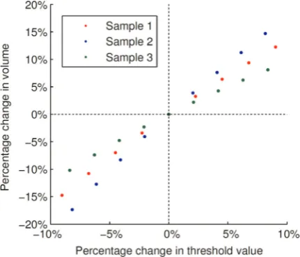
The initial threshold values used to identify the mineral grains were obtained by applying the maximum entropy global thresh-olding algorithm to each rock (Kapur et al., 1985). The threshold was then adjusted from these values and the percentage change in the measured total volume of all the mineral grains calculated (Fig. 3). The shift in threshold value is quantiﬁed using the ratio between absolute shift in the value and the difference between the rock and mineral grain phase thresholds:

T T T T % (1) shift shift grain rock = −

whereTgrainis the threshold for the sulphide grains, andTrockis the

threshold for rock phase. The reason for using the change relative to this difference is that the appropriate threshold value must lie between the intensity of the grains and the matrix.

There is an approximately linear variation in the measured

volume as the threshold value is changed (Fig. 3), though the magnitude of the variation changes somewhat from sample to sample. This variability is probably due to differences in the size distribution of the grains within the three rocks.

The sensitivity of a grain's measured volume to a change in threshold is very dependent on its size relative to the voxel re-solution. Smaller grains are more sensitive to a change in thresh-old because this is mainly a surface effect and smaller grains have a larger speciﬁc surface area. Assuming that a small change in the threshold produces a small change in the location of the boundary (this analysis does not require that the relationship between the change in the position of boundary and the threshold be a simple one, only that the change in position is approximately the same at all boundaries), the fractional change in volume can be expressed as

V V

r r

r kV r (2)

2

3

(1/3)

Δ

∝ Δ = − Δ

whereVis the volume of the grain,ris a linear dimension of the object (proportional toV1/3_{) and}_k_{is a dimensionless constant.}

_Δ

_r is the change in the position of the boundary, which mainly de-pends on the change in the threshold value, but can also depend on the shape and size of the grains. A power law exponent of1/3 implies that the relative change in volume is inversely propor-tional to the grain radius and proporpropor-tional to its speciﬁc surface area.

Plotting

Δ

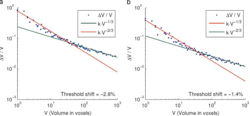
V/Vagainst grain volume for different threshold va-lues (Fig. 4) shows that the larger grains (435 voxels) follow Eq. (2), but that the smaller grains (o35 voxels) have a more ne-gative slope, with_ΔV V/ ₌kV−2/3_{(a power law exponent of} _2/3)

producing a better ﬁt. An exponent of 2/3 implies that the change in the volume upon a threshold change scales with the radius of the grain rather than its area for the smaller grains. This is somewhat unexpected, though possible explanations for this are that either the reconstruction algorithm or the imaging itself is producing more uncertainty in one of the axes than the others. Another possible explanation is that the apparent shapes of some of the objects are strong functions of the threshold value chosen. This is not much of an issue for convex objects, but is likely to be important for more complex objects. For such objects simple thresholding might not be sufﬁcient and more complex techniques may need to be applied. An example of such a method is de-convolution based on an the assumption that the blurring of the edges takes the form of a point spread function (Ketcham, 2006; Ketcham and Hildebrandt, 2014).

While the relative change in the average measured grain vo-lume is of a similar magnitude toTshift(Fig. 3), for individual grains

the difference is strongly size dependent (Fig. 4). Since the small grains are more sensitive to changes in threshold than the larger grains, it is this region of the curve that is most important.

InFig. 5, the prefactor in the bestﬁt to smaller grains (less than 100 voxels) for a power law relationship with an exponent of2/3 is plotted against the change in the threshold value. Since thek value and the magnitude of the average change in volume are directly related, there is also a near linear change ink with the change in the threshold value. This curve will be used later to correct the systematic errors (Section 4).

3.2. Estimation of grain volume uncertainty

[image:4.595.50.266.539.724.2]

While the effect of changing the threshold can be obtained from a single image, repeat scans of the same volume are required to determine the random component of the error. As the scanned volume contains a number of ore particles and each ore particle contains thousands of grains, the identiﬁcation procedure outlined

Fig. 3.The relationship between the change in mineral grain volume and the

variation in the threshold value.

(5)

inSection 2allows us to look at the variability in the measured volume of tens of thousands of individual objects. The same ana-lysis can be carried out for systems containing fewer objects, but in order to generate sufﬁcient statistics on which to base the analysis, repeated scans of the same objects may need to be carried out.

Taking two images of the same sample volume, the relative error in volume measurement for each individual grain was cal-culated. The grain volumes were then ordered according to size and the standard deviation in the relative error was calculated for sets of 500 grains of similar volume and plotted against the mean volume of the set of grains (Fig. 6).

For a single grain the uncertainty (expressed as the standard deviation of the measurement) in the size of the grain is as large as the grain itself for any grain less than approximately 8 voxels. For an uncertainty of less than 10% the grain needs to be larger than about 260 voxels in volume.Fig. 6shows that there is a power law relationship between the standard deviation in the relative error and grain volume, with an exponent of close to 2/3, which is consistent with the scaling for the systematic error1(Fig. 4). This

means that the magnitude of the random component of the error is approximately proportional to the radius of the grain, which is again surprising as the naive expectation would be that this error would be related to the surface area of the grain.

The uncertainty in the measured volume can be reduced by either repeated scans of the same object or by combining the re-sults from a number of similar objects. As the uncertainty for an individual object is a function of the object volume, the number of similar objects, N, of volume V that need to be combined to achieve an acceptable relative error,

ε

, in the measured volume can be calculated (or, alternatively,Nis the number of times that the same object needs to be scanned):

N ( V )

(3) n2

2 κ

ε

=

[image:5.595.88.520.60.261.2]

where

κ

is the prefactor in the relationship between the relative standard deviation in the measure volume of a single grain andn

Fig. 4.The plot of the relative change in grain volume as a function of the volume for two different threshold changes: (a) 2.8% and (b) 1.4%. The power law relationships for

[image:5.595.60.277.296.486.2]

large (1/3) and small grains (2/3) are also shown.

Fig. 5.Plot of prefactorkas threshold value changes.

Fig. 6.Standard deviation in the relative error in the grain volume as a function of

the grain volume.

1

While they have similar volume scalings in this system, there is no funda-mental reason why the systematic and random components of an error need to

(footnote continued) have the same dependencies.

[image:5.595.326.548.299.494.2]

(6)

is the power law exponent. For example, based on the scans used to produce Fig. 6, to reduce the random component of the uncertainty when measuring volume to less than 5% you would need to combine the measurements from approximately 600 grains with a volume of 4 voxels, approximately 12 grains with a volume of 100 voxels, or one object of 1000 voxels (seeFig. 7). This will not account for any genuine variability in the behaviour of nominally identical objects, and it is important to note that it is only the random component of the error that is reduced by averaging repeat results. By deﬁnition, combining results will have no impact on any systematic error.Fig. 7can only be used as an indication of the number of repeats required as this will depend upon the particular material and its scanning conditions.

The procedure presented is relatively straightforward, and is recommended whenever precise quantitative data for the volume or volume change is required.

4. Obtaining consistent results in the face of systematic errors

It is common practice to use intensity standards (usually

introducing the same objects of known attenuation into all scans) when carrying out XMT measurements, and this is usually suffi -cient for samples containing large features with high contrast. In these cases, variations in machine behaviour or beam energy over time (which is equivalent to variations in the threshold value) will be small. However for small objects, especially in low contrast materials or when volume changes can alter the bulk attenuation along the beam path, simple intensity calibration is unlikely to be sufficient. In this case we recommend having both volume and intensity references, especially for smaller grains. The number of reference features needs to be sufficient for suitably accurate vo-lume determination, and the features should not change between scans over a time series experiment. In our particular example of grain dissolution, an appropriate standard could consist of an unaltered particle of the ore that is present in all scans. Ideally this procedure will be carried out using a phantom containing a suf-ficient number of features for which the individual volumes are known, as this will allow not only consistent, but also accurate results. In this specific example the volumes in the reference im-age are not known and thus it is only consistency that is achieved by using this method.

The reason why the correction of systematic errors has been left to last is that it is important to know which errors or dis-crepancies can be eliminated by appropriate adjustment of the thresholds and which errors are random.

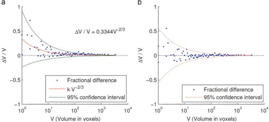
The relative difference in volume (

Δ

V/V) of the grains in two independent scans of the same volume collected under identical machine settings and analysed using the same thresholding al-gorithm (maximum entropy) should be negligible and yet plotting the

Δ

V/Vas a function of grain volume shows a systematic error in the volume, especially for smaller grains (Fig. 8a). The discrepancy between the 2 scans will contain both systematic and random components and therefore the random component is reduced by combining measurements from 100 similar sized grains. This vir-tually eliminates the random component of the error for the larger particles, but it is still signiﬁcant for the smaller particles (below about 100 voxels).

[image:6.595.51.264.58.251.2]

It is expected that much of the systematic difference between the images will be caused by a small inconsistency in the threshold value and it is the smallest grains that have the largest dis-crepancy. The same equation form thatﬁtted the smaller particles inFig. 4is thereforeﬁtted to this data, namely a power law re-lationship with an exponent of2/3.

Fig. 7.Number of repeats required to reduce the random component of the

un-certainty (relative standard deviation) in the volume measurement to a given level as function of the object volume.

Fig. 8.The discrepancy in grain volumes between: (a) a reference scan and a repeated scan of the same ore particle before and (b) after threshold correction (þ1.5% in

relative threshold value).

[image:6.595.74.510.527.724.2]

(7)

Since the expected standard deviation in the average of the 100 grains used to generate each of the points inFig. 8is known from Fig. 6, the 95% confidence interval for thefitted equation can be plotted. For the smaller grains virtually all the pointsfit within this confidence interval, which would be expected if the assumed form for the data is correct. The difference in volume for the larger grains lies outside the confidence interval, but the power law re-lationship with an exponent of 2/3 is only expected tofit the data for the smaller particles.

If there were no systematic error there should be no trend in the discrepancy and the data should be scattered around zero, with a larger scatter at smaller sizes. To try and achieve this, the correction to the threshold required to eliminate the systematic error can be estimated based on the prefactorkin theﬁtted power law (Fig. 8a). The required change in threshold that corresponds to this value ofkcan be obtained fromFig. 5. In this case an increase in the relative threshold value of about 1.5% was required.2_The power law relationship between the change in volume and the volume when the threshold is adjusted means that even this small change has quite a large effect on the smallest grains. If this change in threshold has the same relative effect on the measured volume in the subsequent image as it did on the reference image, then the systematic error should be eliminated.

Fig. 8b shows the discrepancy in the volume once this change in threshold has been applied. It can be seen from the 95% con-ﬁdence intervals that this correction has resulted in discrepancies in volume that are consistent with no systematic error in the size of the smallest grains. While the correction was not based upon the size of the largest grains, the systematic error in their size was reduced from about 2% before correction to 0.8% after correction. The correction has virtually no impact on the random compo-nent of the error, with the relationship between the standard deviation in the measured volume and volume itself for the cor-rected and uncorcor-rected data being virtually the same (seeFig. 6). This indicates that the random and systematic errors are in-dependent of one another in this system. It also means that the random error can be accurately assessed without using a size standard as this component of the error is very insensitive to the speci_ﬁc threshold value used.

5. Conclusions

This paper described methodologies for quantifying, and cor-recting for, both the systematic and random contributions to the uncertainty and error in the measurement of the volume of objects using XMT. In particular, it showed the strong dependency on volume relative to voxel size that these errors have. To achieve a desired level of uncertainty due to random errors, the results from

repeat scans or scans of similar objects need to be combined. The paper showed how many objects of a given size needed to be combined, providing a guide for future studies. For instance a single object of a thousand voxels has an uncertainty of 5% in its volume, while 12 objects of a hundred voxels would need to be combined to achieve the same level of uncertainty. A methodology for eliminating systematic errors based on knowledge of how changes in threshold affect the measured volume and its de-pendency upon size was also developed.

Acknowledgements

This study was performed in the Rio Tinto Centre for Advanced Mineral Recovery at Imperial College London, and at the Man-chester X-ray Imaging Facility, which was funded in part by the EPSRC (EP/I02249X/1). The authors gratefully acknowledge Rio Tinto for their_ﬁnancial support for this project.

References

Aydoğan, N.A., Ergün, L., Benzer, H., 2006. High pressure grinding rolls (HPGR) applications in the cement industry. Miner. Eng. 19, 130–139.

Ghorbani, Y., Becker, M., Mainza, A., Franzidis, J.-P., Petersen, J., 2011. Large particle effects in chemical/biochemical heap leach processes–a review. Miner. Eng. 24, 1172–1184.

Gonzalez, R.C., Woods, R.E., Eddins, S.L., 2003. Digital Image Processing Using MATLAB. Prentice-Hall, Inc., Upper Saddle River, NJ.

Kapur, J.N., Sahoo, P.K., Wong, A.K.C., 1985. A new method for gray-level picture thresholding using the entropy of the histogram. Comput. Vis. Graphics Image Process. 29, 273–285.

Ketcham, R.A., 2006. Accurate Three-dimensional Measurements of Features in Geological Materials from X-ray Computed Tomography Data, Advances in X-ray Tomography for Geomaterials. ISTE, 143–148.

Ketcham, R.A., Carlson, W.D., 2001. Acquisition, optimization and interpretation of X-ray computed tomographic imagery: applications to the geosciences. Com-put. Geosci. 27, 381–400.

Ketcham, R.A., Hildebrandt, J., 2014. Characterizing, measuring, and utilizing the resolution of CT imagery for improved quantiﬁcation ofﬁne-scale features. Nucl. Instrum. Methods Phys. Res. Sect. B: Beam Interact. Mater. Atoms 324, 80–87.

Otsu, N., 1979. A threshold selection method from gray-level histograms. IEEE Trans. Syst. Man Cybern. 9, 62–66.

Puncreobutr, C., Lee, P.D., Hamilton, R.W., Phillion, A.B., 2012. Quantitative 3D characterization of solidiﬁcation structure and defect evolution in Al alloys. J. Met. 64, 89–95.

Stock, S.R., 1999. X-ray microtomography of materials. Int. Mater. Rev. 44, 141–164. Studholme, C., Hill, D.L.G., Hawkes, D.J., 1999. An overlap invariant entropy measure

of 3D medical image alignment. Pattern Recognit. 32, 71–86.

Yue, S., Lee, P.D., Poologasundarampillai, G., Jones, J.R., 2011. Evaluation of 3-D bioactive glass scaffolds dissolution in a perfusionﬂow system with X-ray microtomography. Acta Biomater. 7, 2637–2643.

2

The prefactor in the power lawﬁt to the data inFig. 8(0.3344) is used to read off the required shift in threshold fromFig. 5(1.5%). Note that a positive prefactor implies that the measured volume is too large and that the threshold for the mi-neral grains must thus be increased.