delay systems. In: 2010 American Control Conference ACC 2010,
2010-06-30 - 2010-07-02. ,
This version is available at
https://strathprints.strath.ac.uk/27443/
Strathprints is designed to allow users to access the research output of the University of Strathclyde. Unless otherwise explicitly stated on the manuscript, Copyright © and Moral Rights for the papers on this site are retained by the individual authors and/or other copyright owners. Please check the manuscript for details of any other licences that may have been applied. You may not engage in further distribution of the material for any profitmaking activities or any commercial gain. You may freely distribute both the url (https://strathprints.strath.ac.uk/) and the content of this paper for research or private study, educational, or not-for-profit purposes without prior permission or charge.
Any correspondence concerning this service should be sent to the Strathprints administrator:
The Strathprints institutional repository (https://strathprints.strath.ac.uk) is a digital archive of University of Strathclyde research outputs. It has been developed to disseminate open access research outputs, expose data about those outputs, and enable the
Abstract— A control architecture is proposed for
temperature control in manufacturing applications based on the internal model principle. It is applied to a problem where the material exit temperature is to be controlled by changing the transportation speed to influence the amount of heat loss. The internal model is used to achieve a fast response with minimal overshoot. The controller tuning is carried out using constraints on the sensitivity function to map out the controller parameter region to achieve this performance. The robustness of the controller to parametric uncertainty is also considered. Results are shown from the application of this controller to the temperature controller for a hot strip rolling mill.
I. INTRODUCTION
There are many processes particularly in manufacturing systems where during production the material (metal, glass, paper etc.) is transported from the start of the process to the finish as a continuous web. During transportation the material is loosing heat and the only means to control that heat loss is by varying the speed. The focus of this paper is the control of the process exit temperature using the speed as the primary actuator to adjust the heat lost i.e. if the exit temperature is too low then increasing the speed will reduce heat loss and bring it back on target. These are distributed processes with large transport delays which make the control problem of achieving a fast response with minimal overshoot challenging. Despite the complexity of nonlinear distributed processes we are interested in using a simple linear model and design process to enable controller parameter tuning in the frequency domain.
Using a simple model of a ‘ramp function’ the paper proposes a control architecture using the internal model principle (IMC) with a proportional integral (PI) controller. It is shown how the modeled delay in the internal model can be used as an additional tuning parameter. The optimization of the PI control gains is achieved by mapping constraints on the closed-loop sensitivity function into performance regions for the controller gains. This is extended to plotting the performance regions for multiple models obtained from parametric uncertainty. Results are shown using this controller on a metal rolling mill application. The design model for this application is justified theoretically and from measured data.
G. Hearns is with Converteam Ltd., Boughton Road, Rugby, CV21 1BU, UK (e-mail: [email protected]).
M. J. Grimble is with the Industrial Control Centre, Strathcylde University, 50 George Street, Glasgow, G1 1QE, UK (e-mail: [email protected]).
II. THE RAMP FUNCTION
A simple model to describe the change in temperature with speed for material being transported through a region is the ‘ramp function’ [1]:
(
)
D sT exit
exit
sT e v T v
T − − D
∂ ∂ = ∆
∆ 1
(1)
where TDis the transport delay time and v Texit
∂ ∂
is the steady
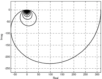
state gain. For a step change in speed the temperature will rise in a ramp of duration TDbefore it reaches steady state. The Nyquist plot of this transfer function shown in Fig. 1 has interesting characteristics. The closed loop system will have multiple poles with the least damped being at low frequency. Of course changing the speed will change the transport delay which is a fixed parameter in this model. The use of the model is limited to ‘small’ changes in speed.
-50 0 50 100 150 200 250 300 -250
-200 -150 -100 -50 0
Real
Im
a
[image:2.595.322.532.377.540.2]g
Fig. 1: Nyquist plot for ∆v to ∆Texit
III. CONTROL ARCHITECTURE
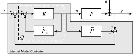
Figure 2 shows the proposed architecture using an internal model in a similar fashion to the Smith Predictor. The output of the plant P(s)is compared to a model of the plant P~(s) which is fed back to be compared with the reference. The output of the PI controller K(s) is fed back through
) ( ~
s
PA in an internal loop. For the Smith Predictor this would
be the delay free model of the plant. For the temperature controller we cannot factorize the plant into a transport delay and the remaining dynamics.
Temperature Control in Transport Delay Systems
P
P
~
K A P~ QFig. 2: Internal model control architecture.
If the internal loop has the transfer function Q
( )
s then the closed loop is:(
)
(
P P)
QrPQ d Q P P Q P y ~ 1 ~ 1 ~ 1 − + + − + −
= (2)
If P~
( )
s =P( )
s and Q( )
s =P~−1( )
s then perfect setpoint tracking and disturbance rejection are achieved. If( )
s P( )
sP~ ≠ then perfect disturbance rejection can still be
achieved, providedQ
( )
s =P~−1( )
s . The Q( )
s is related to the controller and plant model by:K P K Q A ~ 1+
= (3)
When K →∞ then Q→P~A−1. More realistically Kwould only have high gain in the frequency range where disturbance rejection is desired and for a controller with integral actionK
( )
jω →∞,ω→0. The closed loop transferfunction is now:
(
)
P K(
P P)
KrPK d K P P K P K P K P y A A A ~ ~ 1 ~ ~ 1 ~ ~ 1 − + + + − + + − +
= (4)
where:
(
sTD)
D e T s P ~ 1 ~ ~
~= θ − −
(5) and v Texit ∂ ∂ =
θ~ . If we desired the inner control loop Q
( )
s toachieve a faster response we can reduce the transport delay in P~A
( )
s :
(
sTA)
A
A e
T s
P ~ 1 ~
~
~ = θ − −
(6)
where TA TD
~ ~
< . The closed loop can now be written:
(
)
(
)
(
)
(
)
(
e)
KdT s e sT K e T s K e T s e T s y D D A D A T s D sT D T s A T s D T s A − − − + − + − − − + = − − − − − ~ ~ ~ ~ 1 ~ ~ 1 1 ~ ~ 1 1 ~ ~ 1 ~ ~ 1 θ θ θ θ θ (7)
If TA TD
~ ~
= then the internal model structure has no action. Unlike the Smith Predictor the design or tuning of the controller Kis not a delay free problem.
IV. CONTROLLER TUNING
The focus on the controller tuning is to find an appropriate amount of time advance TA
~
and to find gains kP and kI for
the controller: s k k K I P+
= (8)
such that the maximum magnitude of the closed loop sensitivity is less than a preset magnitude:
( )
( )
jw L j S + = 1 1ω (9)
S
( )
jω ≤Msω
sup . (10)
This is equivalent to ensuring that the Nyquist plot of L
( )
jωdoes not intersect with a circle of centre (-1,0) and radius 1
−
s
M [2]. If the circle is represented by a discrete number of
points then we would like to find bounds on kP and kIsuch
that L
( )
jω does not interest with these points. The active bound may be found by finding where L( )
jω is tangential to the circle. For a point u+ jvon the circle, for just a PI control the loop gain is:L
( )
j k jki(
(
P( )
)
j(
P( )
)
)
u jvp− + = +
= ω ω
ω
ω Re Im (11)
With some rearranging we can obtain:
( )
(
)
(
( )
)
( )
2Im Re ω ω ω P v P u P
kp= + (12)
( )
(
)
(
( )
)
(
)
( )
2 Im Re ω ω ω ω P u P v P kI −= (13)
A similar exercise for the IMC PI controller leads to:
( )
( ) (
ω) ( ) (
ω) ( )
ω ω j P jv u j P jv u j P jv u j G A ~ ~ + + + − += (14)
and kP =Re
(
G( )
jω)
kI =−Im(
G( )
jω)
ω (15) As the frequency is varied over the desired design range a region for the control gains is mapped such that the loop gain will not intersect with our design point. With a finite number of design points the final parameter region will be the union of all regions. The active bounds that define the final region may be found by checking the tangency conditions of( )
jωL .
Figure 3 shows the PI parameter region for just the PI control for the process with a 5 sec transport delay and the steady state gain normalized by the corresponding inverse gain in the controller. An additional 1st order lag is added to the plant to represent the dynamics of the speed control. The circle constraint has a radius of 0.8. The parameter region is shown in Fig. 4 for the IMC PI controller whenT~A=T~D 2.
0.2 0.4 0.6 0.8 1 1.2 0.1
0.2 0.3 0.4 0.5 0.6 0.7 0.8
Kp
[image:4.595.77.260.59.383.2]Ki
Fig. 3: PI controller parameter region.
0.5 1 1.5 2 2.5
0 0.5 1 1.5 2
K
p
Ki
Fig. 4: IMC PI controller parameter region.
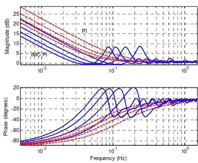
When the transport delay increases the controller parameter region deceases with the optimal integral gain decreasing linearly as shown in Fig. 6. The frequency characteristics of both controllers and the closed-loop sensitivities are compared in Figs 7 and 8 with the transport delay increasing from 5 to 14 secs. The achievable bandwidth of course decreases with the delay increase. The additional phase advance of the IMC PI controller is apparent. The price paid for the extra bandwidth with the IMC PI is the second resonant peak at a higher frequency even although it satisfies the peak constraint.
-0.6 -0.5 -0.4 -0.3 -0.2 -0.1 0 0.1 0.2 0.3 -0.7
-0.6 -0.5 -0.4 -0.3 -0.2 -0.1 0
[image:4.595.325.527.62.219.2]PI IMC PI
Fig. 5: PI and IMC PI loop gain Nyquist plot.
0 0.2 0.4 0.6 0.8 1 1.2 1.4 1.6 1.8 2 0
0.5 1 1.5 2 2.5
Kp
Ki
5 sec
[image:4.595.334.535.245.411.2]8 sec 11 sec 14 sec
Fig. 6: PI and IMC PI controller frequency response.
10-2 10-1 100
0 5 10 15 20 25
M
a
g
n
it
u
d
e
(
d
B
)
10-2 10-1 100
-80 -60 -40 -20 0 20
Frequency (Hz)
P
h
a
s
e
(
d
e
g
re
e
s
)
IMC PI
[image:4.595.330.533.447.614.2]PI
Fig. 7: PI and IMC PI controller frequency response.
10-2 10-1 100
-20 -15 -10 -5 0
Frequency (Hz)
M
a
g
n
it
u
d
e
(
d
B
)
IMC PI PI
Fig. 8: PI and IMC PI controller closed-loop sensitivity.
[image:4.595.85.276.562.712.2]0 2 4 6 8 10 12 14 16 18 20 -1
-0.5 0 0.5
Time (s)
N
o
rm
a
lis
e
d
T
e
m
p
0 2 4 6 8 10 12 14 16 18 20 0
0.5 1 1.5
Time (s)
S
p
e
e
d
(
m
/s
)
IMC PI
[image:5.595.342.522.61.207.2]PI
Fig. 9: Exit temperature and speed.
0.1 0.2 0.3 0.4 0.5 0.6 0.7 0.8 0.9 0
0.05 0.1 0.15 0.2 0.25 0.3
Kp
[image:5.595.337.522.64.384.2]Ki
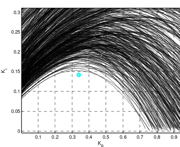
Fig. 10: PI controller parameter region with 50 models.
0.2 0.4 0.6 0.8 1 1.2 1.4
0 0.1 0.2 0.3 0.4 0.5 0.6 0.7 0.8 0.9
K
p
Ki
Fig. 11: IMC PI controller parameter region with 50 models.
The previous design is repeated but now considering 50 plant models that have a 20% variation in the three plant parameters (temperature sensitivity, time delay and speed control time constant). The controller gain region has reduced in size (Figs. 10 and 11) to accommodate the worst case plants but there is still a benefit in using the internal model as illustrated in the closed-loop sensitivity (Fig. 12) and time response (Fig. 13).
10-2 10-1 100
-18 -16 -14 -12 -10 -8 -6 -4 -2 0
Frequency (Hz)
M
a
g
n
it
u
d
e
(
d
B
[image:5.595.65.278.83.275.2])
Fig. 12: PI and IMC PI controller closed-loop sensitivity for 50 models.
0 2 4 6 8 10 12 14 16 18 20
-1 -0.5 0 0.5
Time (s)
N
o
rm
a
lis
e
d
T
e
m
p
0 2 4 6 8 10 12 14 16 18 20
0 0.5 1 1.5
Time (s)
S
p
e
e
d
(
m
/s
)
Fig 13: Exit temperature and speed for 50 models.
Figures 14 and 15 illustrate the effect of varying the time advance used inPA
( )
s~
. With a 30% advance a larger bandwidth can be obtained and with a 70% advance the allowable integral gain is larger. In both these cases the controller response has a large magnitude resulting in excessive actuator energy usage. A good compromise was to use the 50% advance. Using the peak sensitivity constraint only does not give a reliable indication on balancing performance against actuator effort.
0 0.5 1 1.5 2 2.5 3 3.5 0
0.5 1 1.5 2 2.5 3 3.5 4 4.5 5
Kp
Ki
30% Advance 50% Advance
70% Advance
[image:5.595.76.261.274.425.2] [image:5.595.78.265.459.603.2] [image:5.595.331.531.542.698.2]10-2 10-1 100 0 10 20 M a g n it u d e ( d B )
10-2 10-1 100
[image:6.595.77.265.64.216.2]-80 -60 -40 -20 0 20 40 Frequency (Hz) P h a s e ( d e g re e s ) 30% Advance 50% Advance 70% Advance
Fig. 15: IMC PI controller response, varying time advance.
V. ROLLING MILL TEMPERATURE CONTROL
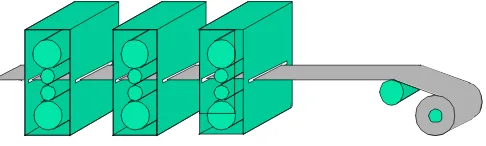
[image:6.595.312.557.428.688.2]Figure 16 illustrates a multi-stand rolling mill where the thickness of the strip (steel or aluminum) is reduced as it passes through each stand before it is coiled. The accurate control of the strip thickness and temperature is essential for profitability [3]. Since the mass flow is constant then the speed of the strip will increase as the thickness is reduced. The exit temperature of the strip from the last stand can be controlled by changing the global speed of the mill and using interstand cooling sprays [4]. Here we only consider using the mill speed as the actuator. Producing strip at the correct exit temperature is important for the metallurgical properties. Getting the strip onto target temperature (with little overshoot or undershoot) as soon as possible will maximize the saleable product.
Fig. 16: Tandem Rolling Mill.
VI. NONLINEAR MODEL
A nonlinear model for the strip temperature is a mill section with respect to time and distance from the mill entry is [4]:
[
]
[
]
in a a T t T x t T T b x t T T a x x t T V t x t T = − + − + ∂ ∂ − = ∂ ∂ ) 0 , ( ) , ( ) , ( ) , ( ) , ( 4 4 (16) Where ch K a C ρ 2 = , ch b ρ σε 2= , T(t,x) is the temperature of the
strip at position x at time t, V is the strip velocity, ρ is the density of the material, c the specific heat, h the thickness of
the material, KC the heat transfer coefficient, Ta the ambient temperature,
ε
is the emissivity andσ
is Stefan-Boltzmann constant.It includes heat loss given by conduction with the atmosphere and heat lost by blackbody radiation. In this paper the radiated heat transfer is ignored (i.e. ε=0). This simplifies the analysis though it is easily extendable to include radiation.
The system has 3 inputs: the entry temperature which is the temperature entering the section, the ambient temperature and velocity. The output is exit temperature from the section. The system has a transport process, which is due to the time it takes for the strip to move though the interstand section. This can be as large as 5-10 seconds. The assumptions made include:
•The temperature of the strip is constant throughout the cross section and only varies along the length of the strip. In reality the centre of the strip will be hotter than the outside.
•It is assumed there is no temperature diffusion along the strip width or length.
•Heat loss through the bottom and top of the strip is equal.
VII. LINEAR MODEL
By linearizing the model with respect to velocity the dependence of the exit temperature on velocity is simplified. It allows a simpler version of the model to be investigated, and analyzed. In particular it allows for frequency responses to be obtained.
The system is assumed to be in steady state initially, i.e. at the steady state temperature, TSS , given byV0, T0 and Tao. The system will remain at this temperature unless the inputs: velocity, entry temperature and ambient temperature change. These changes are given by ∆V, ∆Tand ∆Ta.Therefore the model can be lineraized about any operating point.
(
))
) , ( ) ( ) , ( 0 T T a x t x T V dx x dT V t t x T ao SS ∆ − ∆ + ∂ ∆ ∂ − ∆ − = ∂ ∆ ∂ (17)The steady state temperature, TSSis found by solving this
equation for the steady state i.e. ( , ) =0
∂ ∆ ∂ t t x T and is
(
)
0 0 0 V ax V ax a aoSS T T e T e T
− −
+ −
= (18)
This then leads to the linearized partial differential equation:
(
)
(
)
00 0 0 ) ) , ( ) , ( V ax ao ao e T T a V V T T a x t x T V t t x T − − ∆ − ∆ − ∆ + ∂ ∆ ∂ − = ∂ ∆ ∂ (19)
In this equation the transport delay depends on the steady state velocity, V0 and not the total input velocity,
V V
[image:6.595.58.301.451.524.2]reduces the accuracy for large changes in velocity away from the steady state. The transfer function of the linearized model (19) can now be obtained:
V e
e s V
T T a
T e
s a
a T e
x T
V x s a V
ax a
a V
s a
in V
x s a
∆ −
− −
∆ −
+ + ∆ =
∆
+ − −
+ − +
−
0 0
0 0
) (
0 0
) ( )
(
) (
1 )
(
(20)
where s is the Laplace variable, Xrepresents the Laplace
transform of X and
ch K
a C
ρ
2
= . The values of ∆Tin, ∆Taand
V
∆ independently affect the change in exit temperature. Note that the speed change ∆V conforms to the structure of the ‘ramp function’ in (1). Since the speed of the strip increases as it passes through each stand the transport delay used in the design model is the total transport time from mill entry to exit and the a steady-state sensitivity is calculated to reflect the global behavior.
VIII. APPLICATION RESULTS
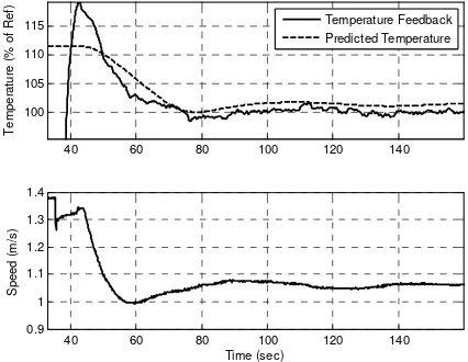
Figures 17 and 18 show some typical results from a multi-stand rolling mill. The initial exit temperature may be either to hot or too cold. When the strip starts to be coiled the temperature control can start adjusting the mill speed. The predicted temperature change due to the mill speed change is shown using the linear model (20) but with a variable transport delay. The model is certainly accurate enough to be used in the IMC PI controller to enable fast but non oscillatory closed-loop responses to be obtained. Using this control structure is also convenient to provide protection for actuator limits such as the maximum acceleration.
40 60 80 100 120 140 100
105 110 115
T
e
m
p
e
ra
tu
re
(
%
o
f
R
e
f)
Temperature Feedback Predicted Temperature
40 60 80 100 120 140 0.9
1 1.1 1.2 1.3 1.4
Time (sec)
S
p
e
e
d
(
m
/s
)
Fig. 17: Exit temperature and speed with a hot strip head.
60 80 100 120 140 160 85
90 95 100 105
T
e
m
p
e
ra
tu
re
(
%
o
f
R
e
f)
Temperature Feedback Predicted Temperature
60 80 100 120 140 160 2
2.2 2.4 2.6 2.8 3
Time (sec)
S
p
e
e
d
(
m
/s
[image:7.595.74.287.493.658.2])
Fig. 18: Exit temperature and speed with a cold strip head.
IX. CONCLUSIONS
It has been shown theoretically and from measured results that a relatively simple transfer function can be used to model the influence of speed on the temperature of a material being transported through a process (particularly a rolling mill process). While the model is simple it does contain a transport delay. An internal model control structure is proposed which uses a model with a reduced transport delay to influence the design problem. The design problem is not delay free and it is therefore convenient to carry out the controller tuning completely in the frequency domain. The bound on the peak magnitude of the closed-loop sensitivity is used to map the feasible region for the proportional and integral gains both for the conventional PI control and the PI control using the internal model. The model, control structure and gain optimization have been successful in practice, providing a simple controller that has high performance.
The effects of the changing speed can be taken into account by using multiple models during the controller design which can also be used to account for other uncertain parameters. This is of course only valid for steady state models and is not a rigorous method for accounting for transients during fast speed changes. It would be interesting for future work to look at the optimal scheduling of controller gains for large changes in speed.
REFERENCES
[1] O. J. Smith, Feedback Control Systems, New York: McGraw-Hill, 1958, pp. 321–323.
[2] K. Astrom and T. Hagglund, PID Controllers: Theory, Design, and Tuning, Instrument Society of America, 1995.
[3] M. J. Grimble and G. Hearns, “Advanced Control for Hot Strip Mills”, Advances in Control (P. M. Frank), Springer-Verlag, 1999. [4] G. Hearns, C. Fryer and P. Reeve, “Finishing Mill Predictive