Boundary layers in pressure-driven flow in smectic A liquid crystals

BOUNDARY LAYERS IN PRESSURE-DRIVEN FLOW IN SMECTIC A LIQUID CRYSTALS∗

I. W. STEWART†, M. VYNNYCKY‡, S. MCKEE†, AND M. F. TOM ´E§

Abstract. This article examines the steady flow of a smectic A liquid crystal sample that is initially aligned in a classical “bookshelf” geometry confined between parallel plates and is then subjected to a lateral pressure gradient which is perpendicular to the initial local smectic layer arrangement. The nonlinear dynamic equations are derived. These equations can be linearized and solved exactly to reveal two characteristic length scales that can be identified in terms of the material parameters and reflect the boundary layer behavior of the velocity and the director and smectic layer normal orientations. The asymptotic properties of the nonlinear equations are then investigated to find that these length scales apparently manifest themselves in various aspects of the solutions to the nonlinear steady state equations, especially in the separation between the orientations of the director and smectic layer normal. Non-Newtonian plug-like flow occurs and the solutions for the director profile and smectic layer normal share features identified elsewhere in static liquid crystal configurations. Comparisons with numerical solutions of the nonlinear equations are also made.

Key words. smectic A liquid crystals, flow dynamics, continuum theory, analytic solution

AMS subject classifications.35Gxx, 65Nxx, 76A15, 76A05, 76Dxx, 76Rxx

DOI.10.1137/140983483

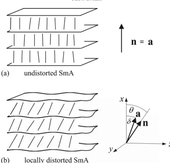
1. Introduction. Nematic liquid crystals generally consist of elongated rod-like molecules that have a preferred local average direction. A unit vector n, called the director, is introduced to describe this average direction of the molecular alignment. Smectic liquid crystals are more ordered than nematics and, for many materials, the smectic phases occur at a temperature below that for which the same material exhibits the nematic phase. The smectic A (SmA) liquid crystal phase occurs when the molecules are arranged within parallel layers where the director is commonly aligned perpendicular to the layers and parallel to the local unit layer normal, a, as shown in Figure 1(a). Further details on the physics of liquid crystals can be found in the books by Chandrasekhar [8] and de Gennes and Prost [12], while more mathematical treatments can be found in the books by Stewart [31] and Virga [35].

The aforementioned depiction of SmA liquid crystals is a rather idealized version of this phase and the model used below will allow for discrepancies between the orientation of the director and the normal to the smectic layers, as shown schematically in Figure 1(b). This is especially relevant in flow problems where the layer normal

∗_{Received by the editors August 22, 2014; accepted for publication (in revised form) June 12,}

2015; published electronically August 26, 2015. This work is part of the activities developed within the CEPID-CeMEAI FAPESP project grant 2013/07375-0.

http://www.siam.org/journals/siap/75-4/98348.html

†_{Department of Mathematics and Statistics, University of Strathclyde, Livingstone}

Tower, 26 Richmond Street, Glasgow, G1 1XH, United Kingdom ([email protected], [email protected]). The third author’s work was supported by a travel assistance grant from the Royal Society of Edinburgh.

‡_{Division of Casting of Metals, Department of Materials Science and Engineering, Royal Institute}

of Technology (KTH), Brinellv¨agen 23, SE-10044 Stockholm, Sweden ([email protected]). This au-thor’s work was supported by a visiting researcher grant within the Government of Brazil’s “Science without Borders” program.

§_{Departamento de Matem´atica Aplicada e Estat´ıstica, Instituto de Ciˆencias Matem´aticas e}

Com-puta¸c˜ao, Universidade de S˜ao Paulo, S˜ao Carlos, SP, Brazil ([email protected]). This author’s work was supported by CNPq–Conselho Nacional de Desenvolvimento Cient´ıfico e Tecnol´ogico, grant 302631/2010-0.

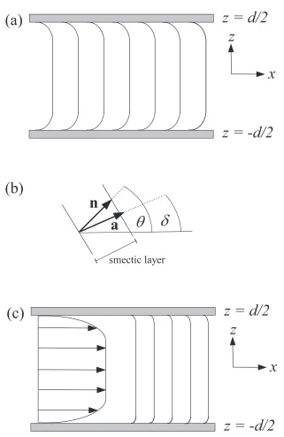
need not necessarily coincide everywhere with the director. A separation between the director and layer normal was considered by Ribotta and Durand [27] and this, together with the sources mentioned in the next section, motivated the nonlinear dynamic continuum theory introduced by Stewart [33] that will be deployed in the problem to be investigated in this article. We consider a sample of SmA liquid crystal confined by fixed parallel planar plates separated at a distancedapart in a bookshelf-type geometry, as shown in Figure 2(a). This figure depicts the anticipated steady state smectic layer structure when a constant pressure gradient is applied in the x -direction, as has been discussed by de Gennes [11] and de Gennes and Prost [12, p. 431] for linearized model equations in the case when nand a are constrained to coincide. Indeed, de Gennes sketches the flow field (see Figure 2(c) and Figure 2(a) in [11]) and argues that the velocity,u, normal to the layers is given by

(1.1) u(z) =−λ_p∂p

∂x

1−cosh(κz) sinh(κL)

,

where λ_p is the permeation coefficient, 2Lis the plate separation distance, andκ= 1/ηλ_p, where κis comparable to the smectic interlayer distance (in the range 20∼ 80 ˚A) and η is the “one-constant” approximation of the viscosity. The purpose of this paper is to clarify and quantify what exactly is happening in this pressure-driven flow when nand a are anchored at the plates. It will transpire that not only does the boundary layer anticipated by de Gennes [11] exist, but another, considerably smaller one affecting n and a also exists; furthermore, it will be shown that these phenomena are particularly sensitive to changes in the magnitudes of the material parameters. Such effects have been reported by experimentalists [5, 6] but it has not previously been possible to capture their qualitative features via previous restricted linear model equations in whichnandaalways coincide. We shall demonstrate how this can be achieved and we shall provide a comprehensive asymptotic analysis of the nonlinear equations; these will be verified and made more precise through numerical computation.

The paper is organized as follows. Section 2 summarizes the dynamic theory, pro-vides a mathematical description of the pressure-driven flow problem, and derives the governing nonlinear dynamic equations. These nonlinear equations are first linearized in section 3 in order to gain a preliminary insight into the steady state problem. It turns out that these equations can be solved exactly for all material parameters; moreover, two physically relevant length scales, given in (3.22) below, can be identi-fied precisely in terms of the material parameters. These length scales will be shown to be directly related to the magnitudes of two physically important boundary layer “distances,” which are in turn connected to the relative reorientations ofnandaand the classical boundary layer “displacement thickness” in relation to the velocity pro-file. A plug-like flow profile occurs in the solution for the velocity. The results derived from the linearized equations allow appropriate rescaled quantities to be introduced and these enable the boundary layers to be estimated when asymptotic and numeri-cal solutions to the nonlinear equations are sought in sections 4 and 5; comparisons between these results will be made and four distinct regions will be identified. The article closes in section 6 with a discussion.

Fig. 1_{. (a)A schematic diagram of locally arranged planar layers of SmA liquid crystal. In}

an undistorted configuration in the bulk, away from any boundary influences, the layers prefer to be equidistant and the local layer normalacoincides with the director n. (b)The layer and director alignments may be perturbed from their preferred undistorted orientations, in which casea andn

need no longer coincide. The orientation angles θand δ, for nand a, respectively, are measured relative to the direction of the undistorted layer normal.

two fixed parallel plates. It will be shown that there are three governing dynamic equations, given below by (2.29), (2.35), and (2.37), and it will be solutions to these equations that will be investigated subject to a symmetry requirement and suitable boundary conditions.

2.1. Dynamic theory. The dynamic theory for SmA liquid crystals formulated by Stewart [33] will be summarized briefly here. Cartesian tensor notation and the summation convention will be used so that any suffix that is repeated precisely twice in an expression is summed from 1 to 3. Partial differentiation with respect to the variablex_j is denoted by a subscriptj preceded by a comma. Following the notation introduced in Figure 1, the smectic layer normalais given by

(2.1) a_i= Φ,i

|∇Φ|, aiai= 1,

because small distortions to lamellar-like layer structures of SmA generally violate this condition.

The directornmust satisfy the constraint

(2.2) n_in_i= 1,

and the incompressibility condition is given by

(2.3) v_i,i= 0,

wherevis the velocity. The rate of strain tensorAand vorticity tensorWare defined in the usual way by

(2.4) A_ij =1₂(v_i,j+v_j,i), W_ij = 1₂(v_i,j−v_j,i),

and, following the standard notation for nematics, the co-rotational time flux N of the directornis defined by

(2.5) N= ˙n−Wn.

A superposed dot represents the usual material time derivative given by

(2.6) D

Dt = ∂ ∂t+vi

∂ ∂x_i.

The general equations that arise from the balance law for linear momentum, in the absence of external body forces and generalized external body forces, are

(2.7) ρv˙_i=−p˜_,i+ ˜g_jn_j,i+|∇Φ|a_iJ_j,j+ ˜t_ij,j,

where ρ is the density, ˜p = p+w_A, where p is the pressure and w_A is the energy density, andJis a “phase flux” term defined by

(2.8) J_i=−∂wA

∂Φ_,i + 1 |∇Φ|

∂w_A ∂a_p,k

,k −∂wA

∂a_p

(δ_pi−a_pa_i).

Note that J is a natural nonlinear extension to the versions discussed in [1, 2, 16, 11, 12]: when it is suitably linearized for small changes in the layer and director orientations, then it reduces to the explicit expressions found in [1, 2] when nand a are allowed to separate. It further reduces to the classical results in [12, 16] when n≡a. The constitutive equations for the viscous stress ˜t_ij and ˜g_i are, respectively,

˜

t_ij =α₁(n_kA_kpn_p)n_in_j+α₂N_in_j+α₃n_iN_j+α₄A_ij

+α₅(n_jA_ipn_p+n_iA_jpn_p) + (α₂+α₃)n_iA_jpn_p

+τ₁(a_kA_kpa_p)a_ia_j+τ₂(a_iA_jpa_p+a_jA_ipa_p)

+κ₁(a_iN_j+a_jN_i+n_iA_jpa_p−n_jA_ipa_p)

+κ₂(n_kA_kpa_p)(n_ia_j+a_in_j)

+κ₃[(n_kA_kpn_p)a_ia_j+ (a_kA_kpa_p)n_in_j]

+κ₄[2(n_kA_kpa_p)n_in_j+ (n_kA_kpn_p)(a_in_j+n_ia_j)]

+κ₅[2(n_kA_kpa_p)a_ia_j+ (a_kA_kpa_p)(n_ia_j+a_in_j)]

and

(2.10) g˜_i =−γ₁N_i−γ₂A_ipn_p−2κ₁A_ipa_p,

where

(2.11) γ₁=α₃−α₂ and γ₂=α₂+α₃.

The above coefficientsα₁ toα₅,τ₁,τ₂andκ₁toκ₆are dynamic viscosity coefficients. The viscosities α₁ to α₅ are nematic-like, while the three viscositiesα₄, τ₁, andτ₂ are analogous to the classical incompressible SmA viscosities [16, equation (3.33)];κ₁ to κ₆ are “coupling” viscosities that are related to the combined effects of nematic and SmA behavior. We remark here that a more extensive theory for SmC [22] has similar contributions.

The balance of angular momentum in the absence of generalized external body forces leads to the equations

(2.12)

∂w_A ∂n_i,j

,j −∂wA

∂n_i + ˜gi =μni,

where μ is a Lagrange multiplier that arises from the constraint (2.2) and can usu-ally be eliminated or evaluated by taking the scalar product of (2.12) with n. The permeation equation is

(2.13) Φ =˙ −λ_pJ_i,i,

where λ_p ≥ 0 is the permeation coefficient. This links the layer flux through a stationary medium to the relevant thermodynamic force [12, 28]. Permeation in locally planar smectics can be thought of as a weak flow of material through the smectic layers in the direction of the local layer normal [20]. This idea was first introduced in the context of liquid crystals by Helfrich [18]. Equations (2.2), (2.3), (2.7), (2.12), and (2.13) provide nine equations in the nine unknowns Φ,n_i, v_i, p, and μ; the smectic layer normalais, of course, determined by (2.1) from the solution for Φ.

One elementary candidate for an energy density is that used by Stewart [33], which has been based upon the one evidently first introduced by Ribotta and Durand [27] and other variants deployed in references [1, 2, 29, 33, 32, 30, 34, 13, 37, 38]. It is given by [33]

(2.14) w_A= 1₂K₁n(∇·n)2+1₂K₁a(∇·a)2+1₂B₀(|∇Φ|+n·a−2)2+₂1B₁1−(n·a)2.

in [1, 2, 29]. AlthoughB₁has been investigated theoretically, measurements for it are scarce in the literature. Nevertheless, Ribotta and Durand [27] have estimated that B₁ B₀. The coupling constantB₁ can alter the critical threshold for the onset of the classical Helfrich–Hurault effect (smectic layer undulations induced by a magnetic or electric field). This has been investigated by Stewart and Stewart [30], where it was shown that for small magnitudes ofB₁the critical field strength for the onset of this effect is lower than that for the classical case, which is recovered as this coupling constant increases: this is indicative of an increased coupling betweennanda. The above model does not exclude the possibility thatnandamay coincide at particular locations or regions.

The nonlinear steady state equations for pressure-driven channel flow will be derived in the next section. When this system of coupled equations is linearized, it turns out that it can be solved explicitly via the theory of linear ordinary differential equations: the most influential material parameters appear to be λ_p, K₁n, and B₁, reflecting the importance of permeation, director distortions, and coupling of the layer orientation to the director; althoughB₀appears in the nonlinear equations, this constant does not appear in the linear equations for a steady state pressure-driven flow. This is a direct consequence of the fact that the coefficient multiplyingB₀is not leading order. The linearized problem is solved in section 3. The solutions from the linear equations will be discussed in relation to known results in the literature. They can also be used for making appropriate comparisons with the asymptotic results and the numerically derived solutions to the nonlinear equations that are investigated in section 4.

2.2. Geometrical set-up and governing equations. Figure 2(a) represents a schematic diagram of a sample of SmA, bounded by planar boundary plates placed a distancedapart atz=±d/2, once a steady state has been reached under the influence of a pressure-driven flow in thex-direction. The orientations ofnandaare described by the angles θ(z) and δ(z), respectively, measured relative to the horizontalx-axis, as shown in Figure 2(b). A non-Newtonian plug-like flow profile is anticipated, based on the earlier work by de Gennes [11], and this is pictured in the notional flow profile shown relative to the local smectic layer arrangement in Figure 2(c). The standard no-slip boundary conditions apply and the SmA layers and the director are assumed to be strongly anchored to the plates, in accordance with the boundary and symmetry conditions. It is therefore supposed that the velocityvis of the form

(2.15) v= (u(z), v(z),0),

where the possibility of a transverse flow component in the y-direction is included (a common phenomenon in nematic liquid crystals [31, 10]). The no-slip boundary conditions are

(2.16) u(±d/2) =v(±d/2) = 0.

Strong anchoring of the director and the smectic layers leads to the boundary condi-tions

(2.17) θ(±d/2) =±θ₀, δ(±d/2) =±δ₀,

Fig. 2_{. (a)A schematic illustration of the anticipated alignment of the SmA layers in a steady}

increases through zero, its second derivative should change from negative to positive withδ(0) = 0 in the center of the sample, where a prime denotes differentiation with respect toz. We are then led to impose the interior symmetry condition

(2.18) δ(0) = 0.

Although this requirement may seem unusual, it proves critical since it enables the solution of the coupled equations derived below. It is also appropriate, and not unex-pected, that the third derivative ofδwill appear naturally in the permeation equation (see (3.2)); as highlighted by de Gennes and Prost [12, p. 411], it is the presence of a third-order derivative that is responsible for the highly anisotropic behavior of such a system.

The director can be set as

(2.19) n= (cosθ,0,sinθ).

Following the technique outlined by Walker [36], we can set the layer function Φ to be

(2.20) Φ(x, z) =x+

z

−d

2

tan(δ(r))dr,

from which it is seen that |∇Φ| = secδ, provided −π/2 < δ < π/2. Furthermore, from the definition in (2.1), it follows that

(2.21) a= (cosδ,0,sinδ),

and, consequently, we have

(2.22) n·a= cos(θ−δ).

Straightforward calculations reveal that N and ˜g, defined in (2.5) and (2.10), are given by

(2.23) N=1₂(usinθ, vsinθ,−ucosθ)

and

˜

g= 1₂γ₁(usinθ, vsinθ,−ucosθ)−1₂γ₂(usinθ, vsinθ, ucosθ) −κ₁(usinδ, vsinδ, ucosδ).

(2.24)

It proves convenient to first examine the equations that arise from the balance of angular momentum given in (2.12). Calculations using the above expressions show that they are

M(θ, δ) cosδ+ ˜g₁=μcosθ, (2.25)

v[ (γ₁−γ₂) sinθ−κ₁sinδ] = 0, (2.26)

M(θ, δ) sinδ+K₁n d 2

dz2sinθ+ ˜g3=μsinθ, (2.27)

where, for notational convenience, the functionM has been introduced as

Equation (2.26) cannot be satisfied for arbitrary nonzero boundary conditions im-posed on θ and δ unless v ≡0. Hence v(z) must generally be a constant and this constant must be zero by the no-slip boundary conditions. There will therefore be no transverse flow in this problem and the velocity reduces tov= (u(z),0,0,). Equation (2.26) is then satisfied automatically. The Lagrange multiplier can be eliminated from the remaining two equations by multiplying (2.25) by sinθ and (2.27) by cosθ and subtracting the resulting expressions. This final step allows the angular momentum equations to reduce to the single equation given by

(2.29)

M(θ, δ) sin(θ−δ)−K₁ncosθ d 2

dz2sinθ+ du dz

α₃cos2θ−α₂sin2θ+κ₁cos(θ−δ)= 0,

where use has been made of the relations in (2.11).

The divergence ofJappears in the linear momentum and permeation equations: however, the evaluation of this divergence will only involve the derivative of the third component ofJbecause of the assumed dependency onzand therefore onlyJ₃needs to be calculated explicitly. We have, from (2.8), that

J₃= cos2δ

K₁acosδ d 2

dz2sinδ+M(θ, δ) sin(θ−δ)

−B₀sinδ[ secδ+ cos(θ−δ)−2 ]. (2.30)

Direct calculations reveal thatρv˙ =0and therefore the linear momentum equations (2.7) become, in an obvious notation,

p_,x=J_3,3+ ˜t_13,3, (2.31)

p_,y= 0, (2.32)

p_,z =−(w_A)_,3+ ˜g_jn_j,3+J_3,3tanδ+ ˜t_33,3. (2.33)

The right-hand side of (2.33) is a function of z only and so we may abbreviate it as G(z). Under the assumption that a constant pressure gradient, a <0, is applied (so that the pressure induced flow is in the positive x-direction), we can identify the pressure from these equations as

(2.34) p(x, z) =ax+

z

−d

2

G(s)ds+p₀,

wherep₀is an arbitrary constant pressure. It is evident that this form for the pressure satisfies (2.32) and (2.33) and so these particular equations can be eliminated from the discussion. Insertion ofp(x, z) into (2.31) leads to

(2.35) a=J_3,3+ ˜t_13,3,

which is the single equation that remains from the linear momentum equations. The only component of the viscous stress that needs to be evaluated explicitly is therefore ˜

t₁₃. Insertingv,n, andainto (2.4), (2.23), and (2.9) gives

˜

t₁₃= 1₂u(α₄+α₅−α₂+τ₂) +1₄uα₁sin2(2θ) +τ₁sin2(2δ) +uκ₁cos(θ+δ) +κ₆cos(θ−δ) + (α₂+α₃) cos2θ +1₂uκ₂sin2(θ+δ) +κ₃sin(2θ) sin(2δ)

The results from (2.30) and (2.36) can be inserted into (2.35) when required for calculations.

It can be verified that the material derivative of Φ, defined in (2.20), with respect to the velocityv= (u,0,0) is ˙Φ =uand so the permeation equation (2.13) becomes

(2.37) u+λ_pJ_3,3= 0.

The three governing equations for this pressure-driven flow are given by (2.29), (2.35), and (2.37), subject to the boundary conditions (2.16), and (2.17) and the requirement (2.18). Before going on to solve these nonlinear equations, it is worth examining the linearized equations in order to identify any potential key material parameters to the problem that may be indicative of characteristic behavior on various length scales or ranges of parameters. The linear equations will be solved analytically to obtain exact solutions. This procedure will be carried out in the next section as a preliminary study prior to obtaining asymptotic and numerical solutions to the nonlinear equations that will be discussed in sections 4 and 5.

3. Linearized equations. Equations (2.29), (2.35), and (2.37) can be linearized under the assumption that the solutionsu,θ, δand their derivatives are small. This leads to the three equations

B₁(θ−δ)−K₁nθ+u(α₃+κ₁) = 0, (3.1)

K₁aδ+B₁(θ−δ) +ηu−a= 0, (3.2)

u+λ_p[K₁aδ+B₁(θ−δ) ] = 0, (3.3)

where, as an abbreviation, we have defined the viscosity coefficientη by

(3.4) 2η=α₂+α₄+α₅+τ₂+ 2 (α₃+κ₁+κ₆).

The viscosity coefficients on the right-hand side of (3.4) tend to zero as the transition to an isotropic fluid takes place, except for the coefficient α₄: the reason for this is analogous to that for the case of smectic C liquid crystals [31, section 6.3.2]. Therefore in the isotropic limit, whennand a are absent, only the usual viscosity for a New-tonian fluid remains, namely, η =α₄/2. This observation will be useful for making comparisons between the results that follow and the well-known results for isotropic fluids.

To simplify the presentation, the approximation K₁n = K₁a will be used since these elastic constants can be considered as being of the same order of magnitude (cf. Auernhammer et al. [2]): the exact solutions can still be found when this approxima-tion is not made but the results become unwieldy and tend to obscure the key roles of various material parameters. Notice also that, using (3.3), (3.2) can be rewritten as

(3.5) ηu−uλ−_p1−a= 0.

The linear system of equations consisting of (3.1), (3.3), and (3.5) can then be written as a matrix system of the form

(3.6) dx

dz =Ax+b,

where the column vectorsx(z) andbare

andAis the 7×7 constant coefficient matrix given by A= ⎡ ⎢ ⎢ ⎢ ⎢ ⎢ ⎢ ⎢ ⎢ ⎣

0 1 0 0 0 0 0

B₁/K₁a 0 −B₁/K₁a 0 0 0 (α₃+κ₁)/K₁a

0 0 0 1 0 0 0

0 0 0 0 1 0 0

0 −B₁/K₁a 0 B₁/K₁a 0 −1/K₁aλ_p 0

0 0 0 0 0 0 1

0 0 0 0 0 1/ηλ_p 0

⎤ ⎥ ⎥ ⎥ ⎥ ⎥ ⎥ ⎥ ⎥ ⎦ . (3.8)

The system (3.6) can be solved exactly. The eigenvalues ofAare±λ₁,±λ₂, and zero, this latter eigenvalue having algebraic multiplicity three, where

(3.9) λ₁= 1

ηλ_p, λ2=

2B₁ K₁a .

The general solution of such a system with a repeated eigenvalue can be determined by constructing a suitable fundamental matrixR(z) [40, p. 582]. The general solution is then

(3.10) x(z) =R(z)c+R(z) z

R−1(s)bds ,

where c = (c₁, c₂, . . . , c₇)T is a constant column vector. The seven components of this constant vector can be determined from the six boundary conditions contained in (2.16) and (2.17) and the requirement (2.18) (recall that v(z) ≡ 0). Explic-itly, we find thatR(z) = Q(z)diag(eλ1z_{, e}−λ1z_{,1, e}λ2z_{, e}−λ2z_{,1,1), where Q(z) is the} matrix

(3.11) Q(z) =

⎡ ⎢ ⎢ ⎢ ⎢ ⎢ ⎢ ⎢ ⎢ ⎣

β₁ β₁ 1 −1 −1 1₂z2+z+ 1 + 2λ−₂2 z+ 1

λ₁β₁ −λ₁β₁ 0 −λ₂ λ₂ z+ 1 1

1 1 1 1 1 1₂z2+z+ 1 z+ 1

λ₁ −λ₁ 0 λ₂ −λ₂ z+ 1 1

λ2₁ λ2₁ 0 λ2₂ λ2₂ 1 0

−λ2₁β₂ λ2₁β₂ 0 0 0 0 0

−λ3₁β₂ −λ3₁β₂ 0 0 0 0 0

⎤ ⎥ ⎥ ⎥ ⎥ ⎥ ⎥ ⎥ ⎥ ⎦ ,

and the constantsβ₁ andβ₂are defined by

β₁= [B1ηλp(α3+κ1−η)−K a

1(α3+κ1) ] η[K₁a+B₁λ_p(α₃+κ₁−η) ] , (3.12)

β₂= (K

a

1)2(λ21−λ22)

ηλ3₁[K₁a+B₁λ_p(α₃+κ₁−η) ]. (3.13)

Applying the conditions (2.16), (2.17), and (2.18) to the solution (3.10) shows that

with

c₁=−asech(λ1d/2) 2λ4₁ηβ₂ , (3.15)

c₄= cosech(λ2d/2) 16B₁K₁aηλ_p(λ2₂−λ2₁)

[ 4B₁(δ₀−θ₀) +ad]

×(2B₁ηλ_p−K₁a)−4aB₁λ32

pη12(α₃+η+κ₁) tanh(λ₁d/2)

, (3.16)

c₇=1

d(δ0+θ0)− ad2 48K₁a (3.17)

+ aλp

K₁adλ₁(η−α3−κ1)(tanh(λ1d/2)−λ1d/2).

These constants allow the solutions forθ,δ, andu, extracted from the solutionx(z), to be written as

θ(z) = 2β₁c₁sinh(λ₁z)−2c₄sinh(λ₂z) +f(z) + az 2B₁, (3.18)

δ(z) = 2c₁sinh(λ₁z) + 2c₄sinh(λ₂z) +f(z), (3.19)

u(z) =aλ_p

cosh(λ₁z) cosh(λ₁d/2)−1

, (3.20)

wheref(z) is the cubic polynomial

(3.21) f(z) =c₇z+ az 12B₁K₁a

B₁6λ_p(η−α₃−κ₁) +z2−3K₁a.

It can be verified directly that these solutions satisfy (3.1) to (3.3) and the boundary conditions (2.16) and (2.17), in addition to fulfilling the requirement (2.18). It is also evident that there are two length scales that are crucial to the behavior of the above solutions, namely,

(3.22) L₁= 1/λ₁ and L₂= 1/λ₂.

The length L₁ coincides with the form of the length scale discussed in [11, 9, 3] and [12, p. 418] and is expected to be of the order of a molecular length (or smectic interlayer distance) when the liquid crystal is in the SmA phase far away from the nematic transition temperature. In this context, we also refer the reader to the related experiments and elementary modeling of permeative flow in SmA by Walton, Stewart, and Towler [39]. The length scaleL₂ is novel and enters through the presence of the coupling constant B₁. For the typical values listed in Table 1, L₁ ∼ 2.4 nm and L₂∼0.25 nm and soL₁is expected to be an order of magnitude larger thanL₂. This discrepancy could potentially lead to the observation of two distinct boundary layer phenomena. The exact solution for ustated above coincides with that given in [11] and [12, p. 430] for a set of linearized flow equations.

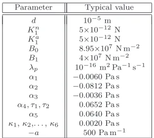
Table 1

Typical material parameters discussed in the text.

Parameter Typical value

d 10−5 m

K₁n 5×10−12N K1a 5×10−12N

B0 8.95×107N m−2

B1 4×107N m−2

λp 10−16m2_Pa−1_s−1

α1 −0.0060 Pa s

α2 −0.0812 Pa s

α3 −0.0036 Pa s

α4, τ1, τ2 0.0652 Pa s

α5 0.0640 Pa s

κ1,κ2,. . . ,κ6 0.0020 Pa s

−a 500 Pa m−1

will be absent, but the solution for u will remain valid in the isotropic limit. It is straightforward to see that taking the appropriate limit asλ_p→ ∞in (3.20) leads to

(3.23) u(z) = a

2η

z2−d 2

4

,

which is the standard parabolic profile for Poiseuille flow. This particular limiting case has also arisen in an application of linear dynamic theory for SmA when it is assumed thatnandacoincide [12, p. 432].

Illustrative examples of the above exact solutions can now be presented for the typical parameter values stated in Table 1 (cf. [12, 31, 34]). Not all of these selected parameters appear in the linearized equations; nevertheless, they will be required for the asymptotic analysis and the numerical calculation of solutions to the non-linear equations in the next two sections. A common value for the sample depth has been set at d = 10μm; experimental set-ups of bookshelf aligned samples of SmA commonly have depths that can be varied between 30μm and 200μm [6] and smectic C samples can have depths from 8μm upward [19]. The elastic constants K₁n and K₁a and the viscosities α₁ to α₅ are based on representative values for the nematic liquid crystal 5CB [31]. The viscosities τ₁, τ₂ are estimates; κ₁ to κ₆ are expected to be lower in magnitude than the other viscosity coefficients as the SmA phase approaches the nematic phase. The value for B₀ is typical for the smectic layer compression constant [31]. The coupling constant B₁ is in accord with the estimates by Ribotta and Durand [27] (B₁ B₀) for SmA and the value for the permeation constant λ_p is that estimated by Kl´eman and Lavrentovich [20, p. 328] (previous measurements forλ_p by Chan and Webb [7] for lamellar bilayers were sub-stantially smaller that this: the value chosen in Table 1 agrees with the experimental evidence reported by Kr¨uger [21], as discussed in [20]). The value for the applied pressure gradient is of the approximate magnitude used experimentally for nematics in [25, 26] when−a=−p_,x∼Δp/L, where Δpcan be of the order 20 Pa andLof the order 35 mm.

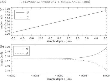
Fig. 3_{.Plots of the exact solutions forθandδprovided by(3.18)and(3.19)using the material}

parameter values stated in Table1whenθ0= 0.2rad andδ0= 0.15rad. (a)Solutions over the full

sample depth−d/2≤z≤d/2. The profile is virtually linear away from the boundaries, as explained in the text. (b) The occurrence of a boundary layer is evident near the boundary at z = d/2, with a similar effect at z = −d/2, by symmetry. The boundary layer is roughly of the order of

L2=

K₁a/2B1∼0.25nm.

represented here, the polynomialf(z) is almost indistinguishable from the orientation angles across the center of the sample and thereforef(z) is a good approximation to θ andδfar from the sample boundaries. Figure 3(b) shows the boundary layer near z=d/2. As expected from the above analysis, this boundary layer is approximately of the order of L₂ = K₁a/2B₁. These results, from the linearized equations, do not exhibit some aspects of the boundary layer behavior that have been reported elsewhere for nonlinear static equations of SmA [32, 36, 13, 14]; the length scale for the boundary layer effect closest to the boundary in the statics of SmA is known [32] to be similarly controlled by a term that is also proportional to 1/√B₁ (albeit in a different context that does not involve flow). For example, there is a greater interplay betweenθand δnear the boundaries which results in novel “competing” preferences in the relative orientations of these angles that are driven by nonlinear contributions to the governing equations (which can also include weak anchoring of the director) and are necessarily absent from the above linear analysis. Such effects were observed to occur over two different length scales in statics: one is clearly similar in form toL₂, but the other cannot be related toL₁since this length scale, which involves viscosity and permeation, can arise only when flow is present.

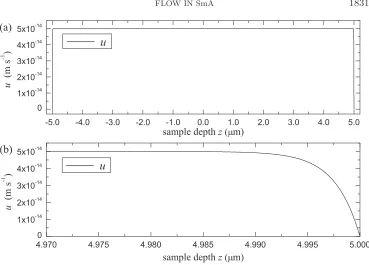
Fig. 4.Plots of the solution forugiven by(3.20), using the material parameters from Table1. (a) The velocity profile for u across the sample −d/2 ≤ z ≤d/2. (b) The boundary layer near

z=d/2; a similar effect occurs atz=−d/2, by symmetry. The boundary layer can be estimated via(3.24)and, in this example, is of the order ofL1=√ηλ∼2.4nm.

“displacement thickness” for fluids near boundaries, defined for semi-infinite samples in [4, p. 311]; such a definition is known to generally underestimate the actual bound-ary layer depth but it does nevertheless provide a rigorous and consistent method of measurement. We find that in this case we may introduce an analogous finite sample depth version as

(3.24) δ∗= 0

−d

2

1−u(z) u(0)

dz= 1

4λ₁cosech 2_(λ

1d/4) (2 sinh(λ₁d/2)−λ₁d),

where the usual upper limit of infinity in the integral version for semi-infinite samples has been replaced by zero, where the maximum value of the velocity, u(0), occurs in a finite sample. It turns out thatδ∗ ∼2.4 nm, which, in this particular example, happens to coincide withL₁=ηλ_p.

The role of L₂ as a dominant length scale for boundary effects is now evident in the solutions for the orientation angles θ and δ, whereas L₁ appears to control the displacement thickness in the velocity profile of u. Two length scales will also be expected to arise naturally when the nonlinear equations are investigated in the context of boundary layer phenomena.

symmetry requirement (2.18). We begin by noticing that (2.35) may be replaced by the equation

(4.1) d˜t13

dz =a+ u λ_p

by substituting for the derivative ofJ₃via (2.37). First, we observe that (2.29), (2.37), and (4.1) are invariant under the transformations

(4.2) u(z) =u(−z), θ(z) =−θ(−z), δ(z) =−δ(−z).

Together with the boundary conditions in (2.16), (2.17) and the interior condition (2.18), this might suggest that we can replace the problem formulated for −d/2 ≤ z≤d/2 with one formulated on 0≤z≤d/2 having the boundary conditions

du

dz = 0, θ= 0, δ= 0, d2δ

dz2 = 0, atz= 0, (4.3)

u= 0, θ=θ₀, δ=δ₀, atz=d/2. (4.4)

Nevertheless, we will not do this here; see the appendix for a discussion on this matter.

4.1. Nondimensionalization. We choose to rescale by setting

(4.5) z∼d, u∼[u],

where [u] =−λ_pa(>0), so that (2.29), (2.37), and (4.1) become, respectively,

cos (θ−δ)−B0

B₁[secδ+ cos (θ−δ)−2]

sin (θ−δ)− K n 1 B₁d2cosθ

d2 dz2sinθ

+ [u] B₁d

du dz

α₃cos2θ−α₂sin2θ+κ₁cos (θ+δ)= 0, (4.6)

B₁λ_p [u]d

d dz

cos2δ

K₁a B₁d2cosδ

d2

dz2sinδ+

cos (θ−δ)

−B0

B₁[secδ+ cos (θ−δ)−2]

sin (θ−δ)

−B0

B₁sinδ[secδ+ cos (θ−δ)−2]

+u= 0, (4.7)

[u]α₄ d2 d dz du dz 1 2

1 + α5 α₄ −

α₂ α₄ +

τ₂ α₄ +1 4 α₁ α₄sin

2_{(2θ) +} τ1 α₄sin

2_(2δ)

+κ1

α₄cos (θ+δ) + κ₆

α₄cos (θ−δ) +

α₂ α₄ +

α₃ α₄

cos2θ

+1 2

κ₂ α₄sin

2_{(θ+δ) +} κ3

α₄sin(2θ) sin(2δ)

+ sin (θ+δ)

κ₄

α₄sin(2θ) + κ₅

α₄sin(2δ) =a+ [u] λ_pu. (4.8)

Set

B= B0

B₁, α¯1= α₁

α₄, α¯2= α₂

α₄, α¯3= α₃

α₄, α¯5= α₅

α₄, ¯τ1= τ₁

α₄, τ¯2= τ₂ α₄,

¯ κ₁= κ1

α₄, κ¯2= κ₂

α₄, ¯κ3= κ₃

α₄, ¯κ4= κ₄

α₄, κ¯5= κ₅

α₄, ¯κ6= κ₆ α₄, (4.9)

where all these are O(1) constants. The parameterB is a measure of the relative influence of the coupling constantB₁ and compression constantB₀; it is known from the analysis of static configurations that a small variation in this control parameter has a high influence onθandδwithin a boundary layer [32]. Equations (4.6) to (4.8) become, respectively,

{cos (θ−δ)−B[secδ+ cos (θ−δ)−2]}sin (θ−δ)

− K1n B₁d2cosθ

d2

dz2sinθ− λ_paα₄

B₁d du dz

¯

α₃cos2θ−α¯₂sin2θ+ ¯κ₁cos (θ+δ)= 0, (4.10)

d dz

cos2δ

K₁a B₁d2cosδ

d2

dz2sinδ+ (cos (θ−δ)−B[secδ+ cos (θ−δ)−2]) sin (θ−δ)

−Bsinδ[secδ+ cos (θ−δ)−2]

− ad B₁

u= 0, (4.11)

−λpα4 d2 d dz du dz 1

2(1 + ¯α5−α¯2+ ¯τ2) + 1 4

¯

α₁sin2(2θ) + ¯τ₁sin2(2δ)

+ ¯κ₁cos (θ+δ) + ¯κ₆cos (θ−δ) + ( ¯α₂+ ¯α₃) cos2θ

+1 2

¯

κ₂sin2(θ+δ) +¯κ₃sin(2θ) sin(2δ)

+ sin (θ+δ) [¯κ₄sin(2θ)+¯κ₅sin(2δ)]

= 1−u. (4.12)

From Table 1, we have

(4.13) λpα4

d2 ∼10

−9_, K1n B₁d2 ∼10

−9_, K1a B₁d2 ∼10

−9_, ad B₁ ∼10

−10_,

which suggests that (4.10) to (4.12) will have boundary layers atz=±1/2 of thickness

(4.14) (K₁n/B₁)1/2/d, (K₁a/B₁)1/2/d, (λ_pα₄)1/2/d,

respectively, i.e., of order∼10−9/2.

4.2. The static case. Consider first the case withu= 0. Denote

(4.15) ε_a = K

a 1

B₁d2, εn= K₁n B₁d2.

Sinceε_a∼10−9, ε_n∼10−9, we choose to set

(4.16) ε_a=ε, ε_n =βε,

whereβ is anO(1) constant; in fact, from the values in Table 1,β= 1. To begin, we first examine the two equations

(4.17) {cos (θ−δ)−B[secδ+ cos (θ−δ)−2]}sin (θ−δ)−βεcosθ d 2

and

d dz

cos2δ

εcosδ d 2

dz2sinδ+ (cos (θ−δ)−B[secδ+ cos (θ−δ)−2]) sin (θ−δ)

−Bsinδ[secδ+ cos (θ−δ)−2]

= 0; (4.18)

the second of these implies that

cos2δ

εcosδ d 2

dz2sinδ+ (cos (θ−δ)−B[secδ+ cos (θ−δ)−2]) sin (θ−δ)

−Bsinδ[secδ+ cos (θ−δ)−2] =C, (4.19)

whereC is a constant that needs to be determined. In the bulk, (4.17) reduces to

(4.20) {cos (θ−δ)−B[secδ+ cos (θ−δ)−2]}sin (θ−δ) = 0,

which implies that either

(4.21) cos (θ−δ)−B[secδ+ cos (θ−δ)−2] = 0 or sin (θ−δ) = 0.

Since the full numerical results indicate thatθ≈δ, we consider the second possibility. Equation (4.19) then implies that

(4.22) −Bsinδ[secδ−1] =C.

The numerics also indicate thatδ1,which would then imply that C1. There is, however, a slight problem: the “small” term

cos2δ

εcosδd 2

dz2(sinδ) + (cos (θ−δ)−B[secδ+ cos (θ−δ)−2]) sin (θ−δ)

(4.23)

was neglected in (4.19), but all that was left were terms which are themselves “small”; in order to keep track of the size of what is being retained or neglected, formal asymptotic expansions forδandθ are therefore required.

A consistent formulation turns out to be possible if we have θ∼ε1/2; thus, we set

(4.24) θ=ε1/2(Θ₀+εΘ₁+· · ·), δ=ε1/2(Δ₀+εΔ₁+· · ·).

At leading order,ε1/2,(4.17) gives

(4.25) Θ₀= Δ₀,

and, using (4.25), atε3/2

(4.26) Θ₁−Δ₁−βd

2_Θ 0 dz2 = 0.

At leading order,ε3/2, (4.19) gives, on using (4.25),

(4.27) d

2_Δ 0

dz2 + Θ1−Δ1− 1 2BΔ

where we have now setC= ¯Cε3/2, where ¯C∼O(1), since the constantCmust be of orderε3/2. Combining (4.25) to (4.27), we have

(4.28) (1 +β)d

2_Θ 0 dz2 −

1 2BΘ

3 0= ¯C.

We will need boundary layers near z = ±1/2. Considering first the boundary layer atz= 1/2, we setz= 1/2−ε1/2Z; (4.17) and (4.18) reduce to just

(4.29) {cos (θ−δ)−B[secδ+ cos (θ−δ)−2]}sin (θ−δ)−βcosθ d 2

dZ2(sinθ) = 0,

cos2δ

cosδ d 2

dZ2(sinδ) + (cos (θ−δ)−B[secδ+ cos (θ−δ)−2]) sin (θ−δ)

−Bsinδ[secδ+ cos (θ−δ)−2] =C, (4.30)

respectively. In this layer,θ, δareO(1), but we need to consider how to match them to the bulk flow, i.e., asZ → ∞. Sinceθ, δ∼ε1/2 in the bulk, we might be tempted just to set

(4.31) θ, δ→0 as Z→ ∞;

however, we should first consider the behavior of Θ₀,Δ₀ asz→1/2. Returning to (4.28), consider the possibility that

(4.32) (1 +β)d

2_Θ0

dz2 ∼ 1 2BΘ

3 0 when

1

2 −z1.

This would imply that

(4.33) Θ₀∼ A

1/2−z,

whereAsatisfies

(4.34) A4 (1 +β)−BA2= 0 ;

the appropriate root for A, which is consistent with the boundary conditions for θ andδin (2.17), is then

(4.35) A=

4 (1 +β) B

1/2 .

Notice also that the form obtained in (4.33) is consistent with the leading-order bal-ance that was assumed in going from (4.28) to (4.32). Next, for the purposes of matching the bulk to the boundary layer flow, we write the bulk solution in terms of the boundary layer variables; thus, at leading order, we have

(4.36) θ=ε1/2Θ₀= A

Z.

limit as Z → ∞, implies that C = 0. In turn, this implies that ¯C = 0; more-over, the fact that d2δ/dz2 = 0 at z = 0 implies that d2Θ₀/dz2 = 0 at z = 0, and hence that Θ₀(0) = 0. With this result, we have shown that, at this order, the solution in θ is antisymmetric, in the manner discussed at the beginning of section 4.

At this stage, the leading-order problem is still not entirely solved, since we have yet to determine the bulk solution completely. Integrating (4.28), we have

(4.37) 1

2(1 +β)

dΘ₀ dz

2 −1

8BΘ 4 0=D

subject to

(4.38) Θ₀(0) = 0

withDa constant to be determined; in addition, (4.33) must be satisfied. It is evident that this must be solved numerically, although solving it as an initial-value problem by starting at z = 0 will fail, because the singular behavior at z = 1/2 will not be resolved; instead, it is necessary to start atz= 1/2 and integrate back toz= 0, with D being iterated for, so as to ensure that (4.38) is satisfied. Settingz= 1/2−ζ, we have

(4.39) 1

2(1 +β)

dΘ₀ dζ

2 −1

8BΘ 4 0=D

with

(4.40) Θ₀(1/2) = 0 and Θ₀∼A

ζ as ζ→0.

Next, set Θ₀=F/ζ so that

(4.41) 1

2(1 +β)

ζdF dζ −F

2 −1

8BF

4_=Dζ4_.

Then

(4.42) ζdF

dζ =F±

BF4+ 8Dζ4 4 (1 +β)

1/2

with

(4.43) F(0) =A and F(1/2) = 0.

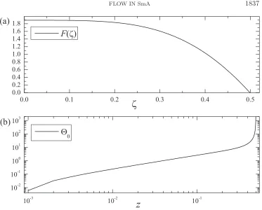
Fig. 5. (a)The dependence ofF uponζ. (b) Θ₀as a function ofz(static case). All that remains is to solve the boundary layer equations; to summarize (after all the simplifications) these satisfy

(4.44) {cos (θ−δ)−B[secδ+ cos (θ−δ)−2]}sin (θ−δ)−βcosθ d 2

dZ2(sinθ) = 0,

cos2δ

cosδ d 2

dZ2(sinδ) + (cos (θ−δ)−B[secδ+ cos (θ−δ)−2]) sin (θ−δ)

−Bsinδ[secδ+ cos (θ−δ)−2] = 0, (4.45)

sinceC≡0 has been established, subject to

(4.46) θ=θ₀, δ=δ₀, atZ= 0 with θ, δ∼ A

Z asZ→ ∞.

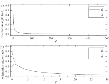
The numerical solutions (computed with COMSOL Multiphysics) for δ and θ are shown in Figure 6; the boundary values have been selected asθ₀=π/6 andδ₀=π/16, these being close to physically realistic data. Figure 6(a) shows the slow algebraic decay ofθ and δ, which is why such a large value of Z_∞, the location of the outer edge of the computational domain, is required. Figure 6(b) showsθ and δ closer to Z= 0; the characteristic hump in δis visible.

4.3. The dynamic case. We now consider what happens whenu= 0. Setting

(4.47) γ=−ad/B₁, ν =λpα4

Fig. 6. The dependence ofθand δupon Z (static case). (a)The domain0≤Z≤500. (b)

A restriction of the result in(a)to the domain0≤Z≤30, which emphasizes the boundary layer effects.

whereγ, ν1, we have

{cos (θ−δ)−B[secδ+ cos (θ−δ)−2]}sin (θ−δ)

−βεcosθ d 2

dz2sinθ+γν du dz

¯

α₃cos2θ−α¯₂sin2θ+ ¯κ₁cos (θ+δ)= 0, (4.48)

d dz

cos2δ

εcosδ d 2

dz2sinδ+ (cos (θ−δ)−B[secδ+ cos (θ−δ)−2]) sin (θ−δ)

−Bsinδ[secδ+ cos (θ−δ)−2]

=−γu, (4.49)

−ν d dz

du dz

1

2(1 + ¯α5−α¯2+ ¯τ2) + 1 4

¯

α₁sin2(2θ) + ¯τ₁sin2(2δ)

+ ¯κ₁cos (θ+δ) + ¯κ₆cos (θ−δ) + ( ¯α₂+ ¯α₃) cos2θ

+1 2

¯

κ₂sin2(θ+δ) +¯κ₃sin(2θ) sin(2δ)+ sin (θ+δ) [¯κ₄sin(2θ)+¯κ₅sin(2δ)]

= 1−u. (4.50)

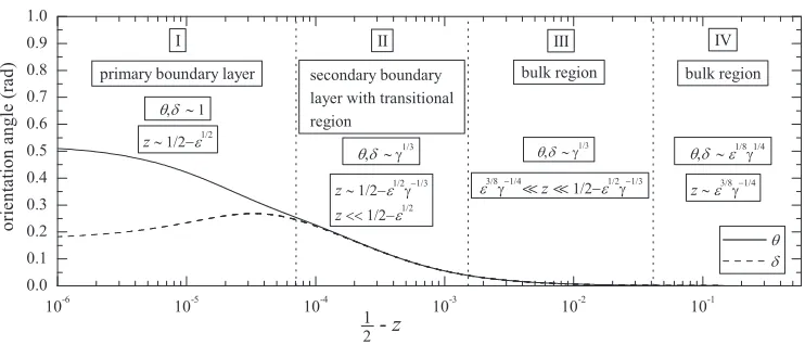
indicated schematically in Figure 9 later. It proves expedient, for calculations in the following subsections, to consider region III first, followed sequentially by regions IV, II, and I.

4.3.1. In the bulk (bulk region III). Consider the leading-order balance of terms for (4.48) to (4.50) in the bulk. Equation (4.50) implies that u ≈1. Noting that ε, γ, ν are more or less the same order of magnitude, i.e., 10−9−10−10, the leading-order balance for (4.48) gives the same result as did (4.17), i.e., θ≈δ. The major difference between the static and dynamic cases arises in (4.49). Suppose that δ∼O([δ]), where [δ] is to be determined, although clearly [δ]1. Equation (4.49) has terms with magnitudes

(4.51) ε[δ], [δ]3, γ .

Consider, in turn, the possible leading-order balances in (4.49):

1. The balance used for the static case, [δ]∼ε1/2, is no longer valid here, since ε3/2γ.

2. We cannot haveε[δ]∼γsinceγ/ε∼O(1), whereas we must have [δ]1. 3. The only remaining possibility is [δ]3 ∼γ, which implies [δ]∼γ1/3. This is

feasible sinceεγ2/3. By setting

(4.52) θ=γ1/3

Θ₀+γ1/3Θ₁+· · ·

, δ=γ1/3

Δ₀+γ1/3Δ₁+· · ·

,

(4.48) gives, at leading order, O(γ1/3) and Θ₀−Δ₀ = 0. Equation (4.49) gives, at leading order,O(γ), noting thatεγ1/3γ,

(4.53) d

dz

1 2BΘ

3 0

= 1,

whence

(4.54) Θ₀= Δ₀=

2z+A∗₊ B

_1/3

,

where A∗₊ is a constant to be determined. For z < 0, there is something similar, namely,

(4.55) Θ₀= Δ₀=

2z+A∗₋

B

_1/3

.

4.3.2. Boundary layer at z = 0 (bulk region IV). However, it is evident that Δ₀ will not satisfy the boundary condition at Δ₀(0) = 0, and so we need a boundary layer there. Suppose it is of thickness [z]. We set

(4.56) z= [z]Z, Θ₀= [Θ₀] ¯Θ₀, Δ₀= [Δ₀] ¯Δ₀,

where [z],[Θ₀], and [Δ₀] are scales to be determined, although we expect

(4.57) [z], [Θ₀], [Δ₀]1.

Assume for the moment that the leading-order balance in (4.48) leads to

which implies that [Θ₀] = [Δ₀] and

(4.59) Θ¯₀= ¯Δ₀.

Furthermore, from (4.49),

(4.60) 1

[z] d dZ

−εγ1/3[Δ0] [z]2

d2Δ¯₀ dZ2 +

γ[Δ₀]3

2 B

¯ Δ3₀

=γ .

Thus, to retain all terms in (4.60), we need

(4.61) εγ

1/3_[Δ 0]

[z]2 =γ[z] =γ[Δ0] 3_,

and hence

(4.62) [z] =ε3/8γ−1/4, [Δ₀]∼ε1/8γ−1/12

(and consequentlyθ, δ∼γ1/3[Δ₀] =γ1/3[Θ₀], i.e.,θ, δ∼1/8γ1/4). We are therefore left with

(4.63) d

dZ

−d2Δ¯0 dZ2 +

1 2B

¯ Δ3₀

= 1,

and so

(4.64) −d

2_Δ¯₀

dZ2 + 1 2B

¯

Δ3₀=Z+A,

whereA is a constant to be determined. For correct matching asZ → ±∞, we need A∗_± = 0. To see this we first observe from (4.64) that ¯Δ₀∼(2Z/B)1/3when Z 1. However,

(4.65) Δ₀= [Δ₀] ¯Δ₀= [Δ₀]

2[z]z B

1/3 =

2Z B

1/3 ,

and so we deduce thatA∗_±= 0.

Equation (4.64) now remains, subject to the requirements

(4.66) d

2_Δ¯₀

dZ2 = 0 atZ = 0, and ¯ Δ₀∼

2Z B

1/3

asZ→ ±∞,

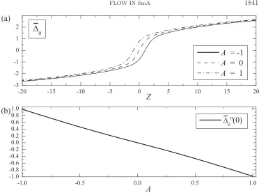
which can be solved numerically. Figure 7(a) shows ¯Δ₀ versus Z for A = −1,0,1 and Figure 7(b) shows ¯Δ₀(0) versus A; clearly, the requirement that ¯Δ₀(0) = 0 necessitates thatA= 0.

However, we should check that the assumption that led to (4.54) was correct. For this, we require that

(4.67) γ1/3[Θ₀] εγ

1/3_[Θ 0] [z]2 ,

Fig. 7. (a)The dependence ofΔ¯₀uponZforA=−1,0, and1. (b)The dependence ofΔ¯

0(0)

uponA.

4.3.3. Transition layer (secondary boundary layer II). Again, we will need boundary layers near z=±1/2. First, we will needθ, δ ∼γ1/3, so as to be able to match to the bulk. Set z= 1₂−[z]ζ. The orders of magnitude of the relevant terms in (4.49) are

(4.68) εγ

1/3

[z]3 , γ2/3

[z] , γ [z], γ .

This time, not all terms can be accommodated, since [z] 1, so the leading-order balance must be between the first and the third term; thus,

(4.69) εγ

1/3

[z]3 ∼ γ

[z] =⇒[z] =ε

1/2_γ−1/3_.

Setting

(4.70) z=1

2 −ε

1/2_γ−1/3_{ζ, δ=γ}1/3_{Δ, θ=γ}1/3_Θ,

(4.48) and (4.49) give, at leading order,

Δ = Θ, (4.71)

d dζ

d2Δ dζ2 −

1 2BΔ

respectively, with

(4.73) Δ→

1 B

_1/3

as ζ→ ∞.

Note that asζ→ ∞,Δ must tend to Δ₀ in the bulk (given by (4.58)) asz→ 1₂. Note incidentally that the first term and last terms on the left-hand side of (4.48) are of orderγ1/3andγ2/3ε−1/2ν, respectively. However, sinceεandν are of the same order of magnitude in this problem, we use the fact thatε3/2 γ to conclude that γ1/3 γ4/3ε−1/2ν, which then leads to (4.71). Also, observe that the terms that have been retained in (4.72) from the original equation (4.49) are of orderγ4/3ε−1/2, whereas the term on the right-hand side of (4.49) is of orderγ. Again, we useε3/2γ to see thatγ4/3ε−1/2γ.

Equations (4.72) and (4.73) then lead to

(4.74) d

2_Δ

dζ2 − 1 2BΔ

3₌₋1 2.

Observe the similarity between (4.74) and (4.32) in the “static” case; in particular, we can note that, forζ1, Δ∼A/ζ withA(2−1₂BA2) = 0. Selecting the positive root then implies that

(4.75) Δ∼

4 B

1/2 ₁

ζ.

Now, we have, on multiplying (4.74) by dΔ/dζ, integrating, and using (4.73),

(4.76) 1

2

dΔ dζ

2 −1

8BΔ 4₌₋1

2Δ + 3 8

1 B

1/3 .

To solve (4.76) numerically, set Δ =G/ζ so that

(4.77) ζdG

dζ =G−

1

4BG4−ζ3G+ 3 4

1 B

_1/3

ζ4,

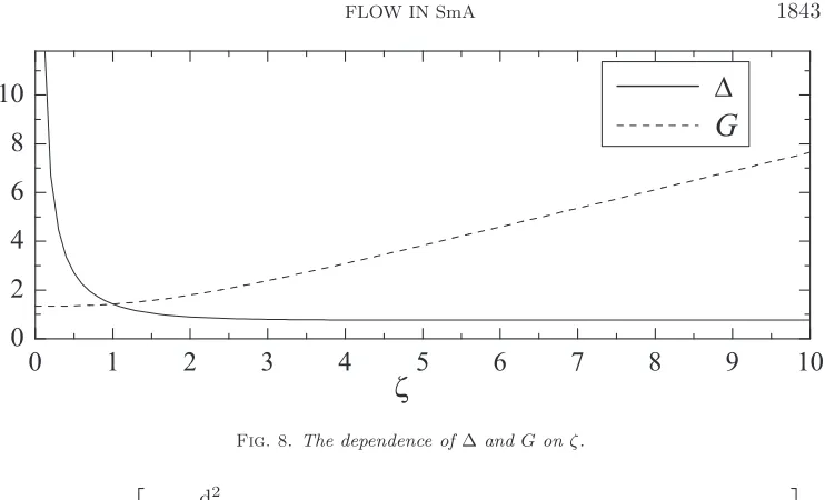
again selecting the positive root, subject to G(0) = (4/B)1/2. Solving forG numeri-cally, we obtain the profile for Δ as shown in Figure 8, which also shows the function G. Observe also that sinceν ε1/2γ−1/32, (4.50) simply reduces tou= 1 in this layer, as in the two bulk regions.

4.3.4. Boundary layer at z = 1₂ (primary boundary layer I). However, Δ (and Θ) as determined above still cannot satisfy the boundary conditions at z = 1/2. For this, we need a sublayer where θ, δ ∼ O(1) and ₂1 −z ∼ ε1/2; setting z= 1/2−ε1/2Z, (4.48) and (4.49) reduce, at leading order, to just

(4.78) {cos (θ−δ)−B[secδ+ cos (θ−δ)−2]}sin (θ−δ)−βcosθ d 2