Testing the effects of gravity and motion on quantum entanglement in space-based experiments

This content has been downloaded from IOPscience. Please scroll down to see the full text.

Download details:

IP Address: 130.159.82.88

This content was downloaded on 08/08/2014 at 10:45

Please note that terms and conditions apply.

Testing the effects of gravity and motion on quantum entanglement in space-based

experiments

View the table of contents for this issue, or go to the journal homepage for more 2014 New J. Phys. 16 053041

entanglement in space-based experiments

David Edward Bruschi1, Carlos Sabín2, Angela White3,6, Valentina Baccetti4, Daniel K L Oi5and Ivette Fuentes2

1_{School of Electronic and Electrical Engineering, University of Leeds, Woodhouse Lane, Leeds}

LS2 9JT, UK

2_{School of Mathematical Sciences, University of Nottingham, University Park, Nottingham}

NG7 2RD, UK

3_{Joint Quantum Centre (JQC) Durham-Newcastle, School of Mathematics and Statistics,}

Newcastle University, Newcastle upon Tyne NE1 7RU, UK

4_{School of Mathematics, Statistics and Operations Research, Victoria University of Wellington,}

PO Box 600, Wellington 6140, New Zealand

5_{SUPA Department of Physics, University of Strathclyde, Glasgow G4 0NG, UK}

E-mail:[email protected]

Received 22 August 2013, revised 14 April 2014 Accepted for publication 17 April 2014

Published 21 May 2014

New Journal of Physics16(2014) 053041 doi:10.1088/1367-2630/16/5/053041 Abstract

We propose an experiment to test the effects of gravity and acceleration on quantum entanglement in space-based setups. We show that the entanglement between excitations of two Bose–Einstein condensates is degraded after one of them undergoes a change in the gravitational field strength. This prediction can be tested if the condensates are initially entangled in two separate satellites while being in the same orbit and then one of them moves to a different orbit. We show that the effect is observable in a typical orbital manoeuvre of nanosatellites like CanX4 and CanX5.

Keywords: quantum entanglement, relativistic effects, space-based experiments

6

Current address: Quantum Systems Unit, Okinawa Institute of Science and Technology Graduate University, Onna-son, Okinawa 904-0495, Japan.

1. Introduction

Quantum mechanics and relativity are the two most fundamental theories of the universe known to science. Despite both working extremely well in predicting and quantifying effects in their respective regimes of application, they are commonly deemed as incompatible. On one hand, quantum mechanics predicts with great accuracy the behaviour of microscopic particles that can be in a superposition of being in two different places at once. On the other hand, general relativity provides an effective description of the universe at large length scales where time can

flow at different rates in different places. However, we do not fully understand what happens when these effects occur together. The inability to unify these theories remains one of the biggest challenges in theoretical physics today.

Understanding general relativity at small length scales where quantum effects become relevant is a highly non-trivial endeavour that has suffered from a lack of experimental guidance. An alternative approach is to study quantum effects at large scales, which promises to be experimentally achievable in the near future [1, 2]. Cutting-edge quantum experiments are reaching relativistic regimes, where the effects of gravity and motion on quantum properties can be experimentally tested. In 2012 a teleportation protocol was successfully performed across 144 km by the group lead by Zeilinger [3]. Motivated by this success and related experimental developments [4–6], major space agencies, e.g. in Europe and Canada, have invested resources for the implementation of space-based quantum technologies [7–9]. There are advanced plans to use satellites to distribute entanglement for quantum cryptography and teleportation (e.g. the Space-QUEST project) and to install quantum clocks in space (e.g. the Space Optical Clock project). Such experiments are of great interest since relativistic effects can be expected at the regimes where satellites operate. For instance, it is well-known that the global positioning system (GPS), a system of satellites used for time dissemination and navigation, requires relativistic corrections to determine time and positions accurately. Indeed previous theoretical work has addressed these fundamental questions by showing that gravity, motion and space-time dynamics can create and degrade entanglement [10]. For instance, recent work [11] shows that acceleration produces observable effects on quantum teleportation. However, current experimental space-based designs are yet to consider thesefindings. In this paper we propose a space-based experiment to test the effects of gravity and motion on quantum entanglement.

Most proposals to implement quantum technologies in space have been developed within the framework of quantum mechanics [12]. However, quantum mechanics is a non-relativistic theory where the effects of acceleration and gravity can only be addedad hoc. The correct arena in which to look for relativistic effects is quantum field theory (QFT), which describes the behaviour of quantum fields in space-time. It is a semiclassical description in the sense that mater and radiation are quantized but the space-time is treated as a classical background. However, unlike quantum mechanics, QFT naturally incorporates Lorentz invariance, as required by the postulates of relativity theory. Indeed, QFT successfully merges quantum theory and special relativity in the framework of the standard model of elementary particles. Moreover, QFT in curved spacetime provides some answers to questions about the overlap of quantum

mechanics and general relativity [13]. Very recently we have started to see some of its

correctly account for effects that take place at increasing length and shorter time scales, quantum information must be extended to a fully relativistic setting.

In this paper we use a QFT framework to show that the gravitationalfield of the Earth and accelerated motion can induce experimentally observable effects on the basic resource for

quantum information and communication tasks, namely quantum entanglement. Our findings,

on the one hand, shed light on fundamental questions about the overlap of quantum theory and relativity and, on the other hand, will enable experimentalists to correct negative gravitational effects on quantum information. Our research programme aims not only to characterize relativistic effects so that they can be corrected, but also to learn how to exploit them in order to improve the performance of quantum technologies in space.

Recently, it has been shown that the entanglement between field modes of localized

[image:4.595.135.448.115.385.2]

systems, such as cavities, is sensitive to changes in acceleration [18]. Via the equivalence principle, this means that entanglement should, therefore, be affected by changes in gravitational field strengths. We propose to demonstrate this experimentally by considering the entanglement between the excitations of two Bose–Einstein Condensates (BECs), each one of them prepared in a separate satellite. The BEC excitations we consider are known as quasiparticles or phonons. These excitations obey, under certain circumstances, a massless Klein–Gordon equation with a very slow speed of propagation [19]. Low propagation speed is the key element to enable the observation of the effect we describe below within realistic experimental regimes. We propose to entangle two BEC modes, one in each BEC, while the BECs move close to each other along the same circular Earth orbit. One of the satellites will

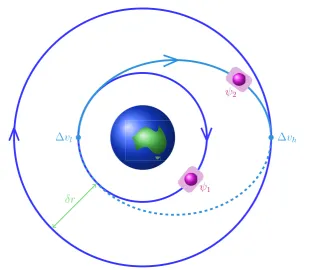
then undergo non-uniform motion to change to an orbit subject to a different gravitationalfield strength (seefigure1). Our analysis shows that the entanglement degradation between the BEC modes is a periodic function of the change in gravitationalfield strength in the orbit. This effect is already significant for typical parameters involved in microsatellite manoeuvres, which is a great advantage since experiments involving such satellites have relatively low costs.

2. Model and results

Let us explain our methods and results in more detail. In the absence of atomic collisions, a BEC can in principle reach absolute zero temperature and be described by a classical mean

field. However, collisions are always present and therefore, in the superfluid regime, the condensate is better described by a meanfield classical background plus quantumfluctuations. The fluctuations, for length scales larger than the so-called healing length, behave like a phononic quantumfield. The classical background energy density, pressure and number density play the role of an effective spacetime metric which in principle can be curved. The dependence of this metric on the BEC parameters will be presented below. ThefieldΠ ξ

( )

can be expanded in terms of the so-called Bogoliubov modesϕ ξ

( )

[19],

∑

Π ξ

( )

=

(

ϕ ξ

( )

a + ϕ*

( )

ξ a†

)

. (1)

k

k k k k

We useξto denote arbitrary coordinates. The operatorsa_kanda_k†associated with the modes are annihilation and creation operators, respectively, which obey the standard canonical commutation relations. The dispersion relation is given by ω_k = c_s k where c_s is the speed of sound.

In a homogenous condensate, the modes obey a massless Klein–Gordon equation□Π= 0

where the d’Alembertian operator □ = 1 −g ∂_a

(

−g gab∂_b

)

depends on an effective

spacetime metricg

ab, with determinant g given by (see appendix A): [20, 21]

g ⎛

⎝

⎜ ⎞

⎠ ⎟⎡

⎣ ⎢ ⎢

⎛ ⎝

⎜ ⎞

⎠

⎟ ⎤

⎦ ⎥ ⎥

ρ

=

+ + −

− n c

p g

c c V V

1 . (2)

ab

s

ab

s a b

0 2 1

0 0

2

2

Note that this metric is a function of the background meanfield properties of the BEC such as the number density n₀, the energy density ρ₀ and the pressure p₀. The effective curvature

naturally arises from decoupling the field equations of the background mean field and the

quantum fluctuations.V_a is the BEC 4-velocity with respect to the laboratory reference frame,

while g

ab is the background, real spacetime metric that in general may be curved. Strictly

suitable to describe periods of uniformly accelerated motion (see appendixB). We choose the comoving frameV_a =

(

c; 0, 0, 0

)

since we want to describe the effects in the rest frame of the BEC. Under these conditions we obtain an effective metricg

ab which is also conformally flat

(see appendixA).

For the sake of simplicity, we consider a quasi one dimensional BEC. Suitable close to hard-wall boundary conditions [22–24], this allows us to consider a spectrum similar to the well-known spectrum of an optical cavity given byω_n = 2π × n c

L

s_{, where Lis the length of the}

cylinder. Initially, two space experimentalists, Valentina and Yuri, prepared a two-mode squeezed state between two inertial BECs with squeezing parameterr > 0. Details on how to prepare such a state are discussed in appendixC. The quantum correlations of this state are fully characterized by the reduced covariance matrix of the two modesσ_kk′, a real 4 × 4 matrix that only depends on r (see appendix C). In particular, entanglement can be quantified with the negativity which for this state is given by [25]

⎡

⎣⎢ ⎤⎦⎥

=

(

−

)

N max 0, 1 e

2 1 , (3)

( )0 2r

where the condensate undergoes free evolution. After preparing the initial state, Yuri moved his BEC into an orbit subject to a different gravitational potential. This is achieved by accelerating with constant accelerationafor a proper timeτas measured by an observer at the centre of the rigid trap [26]. Once in the new orbit, the BEC moves inertially again. It is important to make sure that the motion preserves the homogeneity of the condensate. In principle, the acceleration can make the condensate become inhomogeneous. However, these effects are negligible in the regimes considered in our discussion (see appendix B). The initial covariance matrix σ of the state including all modes is transformed after the change in orbit into σ˜ = S Sσ T, where S is a symplectic matrix that encodes the time evolution of the system. The reduced covariance matrix

σ˜_kk′for the two particular modeskandk′of interest can be obtained fromσ˜. During inertial and

uniformly accelerated segments of motion, the field modes only undergo free evolution.

Therefore, the transformation in this case is simply composed of local rotations with anglesω_kt

and ω_k′t, where ω_k and ω_k′ are the angular frequencies of the modes k and k′ respectively. However, during changes from inertial to accelerated motion, the modes undergo a Bogoliubov transformation with coefficients ₀α_mn and ₀β_mn that relate the mode functions in the Minkowski and Rindler frames [27]. The coefficients ₀α_mn account for mode mixing within the moving

condensate, while β

mn

0 account for particle pair production. Therefore, the total Bogoliubov

coefficients α_mn, β_mn are functions of ₀α_mn, ₀β_mn and of phases acquired during the period of uniform acceleration. They can be computed analytically (see appendixC) using a perturbative expansion in the parameter:

= ≪

h a L c_s2 1 . (4)

We can write the coefficients as α_mn = α_mn( )0 + α_mn( )1h + O h

( )

2 _{and β = β h + β h}

mn mn mn

2 ( )1 ( )2

+O h

( )

3 . After the change of orbit, we find that the entanglement has changed and is

⎡

⎣ ⎤⎦

= − α + β − β

′ ′ ′

(

(

)

)

N max 0, N( ) 1 er f f h e f h , (5)

k k

r k

0 2 2 2 2

where α

′ f_k, β

′

f_k are functions of the Bogoliubov coefficients that depend periodically on the difference of gravitationalfield strength (see appendixC). Note thatN( )0 is the entanglement of the initial state given by equation (3). Nis always smaller than N( )0, since the entanglement is degraded by mode mixing and particle creation [14, 11]. This degradation effect becomes observable for large enough, but still perturbative, values of h, h2 ≃ 0.05 [11]. In optical cavities, these values ofhare obtained with accelerations of10 m s23 −2 (see equation (4)) while in superconducting cavities, the corresponding order of magnitude is10 m s17 −2, which can be achieved by non-mechanical means [14, 11]. In the case under study here namely, BECs, the typical valuesL ≃ 100 mμ andc_s = 1 mm s−1 give rise toa ≃ 10−3m s−2.

3. Experimental setup

We now assess the feasibility of testing the degradation of entanglement due to orbit changes with a space-based experiment using a pair of nanosatellites. Nanosatellites are fully functional spacecraft with a mass of 1–10 kg. The use of conventional off-the-shelf parts, component miniaturization, and standardized systems means that they are a comparatively low cost avenue to space. Capabilities such as power, attitude and position control, propulsion, optics, communication, and autonomous operation are under active development, which greatly expands the missions that may be undertaken within the mass and volume envelope of the nanosatellite platform. At the same time, quantum experiments have also become more compact which makes it feasible to place them on small satellites [6].

An example of the capability required for such an experiment is the pair of CanX 4 and CanX 5 [28,29] satellites due to have launched in 2013. These are built according to the generic

nanosatellite bus specification which consists of a 20 cm a side cube with a mass of

approximately 7.5 kg. Typically, such a spacecraft will have a mission payload volume of 1.8 litres and mass of 2 kg. The CanX 4/5 pair will demonstrate formation flying in orbit and are each equipped with high precision differential GPS receivers for cm relative positioning determination, and a single axis thruster allowing orbit changes. The latter consists of the Canadian Nanosatellite Advanced Propulsion System and has a rated thrust of20 mNand anI_sp

thermal state instead of the vacuum state, the amounts of initial squeezing and entanglement that can be generated will be lower [33]. In order to generate a squeezing of r = 1 2 at frequencies of100 Hz, the BEC should be cooled down to a few nK. Finally, notice that the experimental setup required to create and hold the BEC can be as small as 0.5 L [34]. Important efforts are currently taking place to load and maintain a BEC on a chip device in space. See, for example, the QUANTUS project [35] aimed at using a BEC to detect microgravity effects in space.

The effects predicted in this work arise when a satellite undergoes a change of circular orbit, determined by the difference in gravitationalfield strength between the initial and final orbits. As an example, the change of orbit can be achieved in an efficient and elegant manner by means of a Hohmann transfer orbit [36,37] (seefigure1). The procedure is the following. First a change of velocityΔv_l moves the satellite to an elliptic orbit. Then the satellite navigates half of this new orbit, beforefinally a second velocity kickΔv_h puts the satellite back into a circular orbit. The difference between the radius of the initial orbitr_l and the radius of thefinal orbitr_h

determines the magnitude of the velocity kicks through the relations

⎛ ⎝

⎜ ⎞

⎠ ⎟

⎛ ⎝

⎜ ⎞

⎠ ⎟

Δ

Δ

=

+ −

= −

+

v GM

r

r

r r

v GM

r

r

r r

2

1

1 2 , (6)

l

l

h l h

h

h

l l h

where G is Newtonʼs gravitational constant and M is the mass of the earth. In

particular, assuming a small change of altitude r_h = r_l + δ r with δ r ≪r_l, we find

Δv_l ≃ Δv_h ≃ GM δ ≃ δ ϕ ≃ 3 10 m s− −

r r r

r GM

4 4

3 1 h h

h _{for a low Earth orbit (LEO) of}

= +

r_h R_e 400 km—R_e being the radius of the Earth and δ ϕ the difference in gravitational

field strength between the initial and final orbits. Therefore, for constant acceleration, each radial distance between circular orbits is related to a different duration of the acceleration. The

whole manoeuvre takes a half-period P 2 of the elliptical transfer orbit

π

≃ ≃

P 2 r GM_h3 5000 s, which is larger than the average lifetime of a BEC. However, the degradation of the entanglement takes place immediately after thefirst change in velocity, and can be observed during the navigation of the transfer orbit. Equations (5), (6) imply that the

entanglement oscillates with the radial distance between the initial and final orbit, or

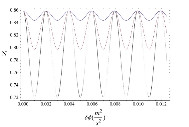
equivalently, with the difference in the gravitational strength. In figure 2 we show that, for realistic experimental parameters, oscillations have a significant amplitude and a period of around 2 m, meaning that almost any change of orbit would lead to an observable effect on the initial quantum entanglement. Note that the duration of the acceleration in the plot is of the order of 0.1 s. The maximum change of velocity is Δv_l ≃ 10−3m s−1, well within the reach of current technologies since CanX4 and CanX5 are capable of achieving maximum changes of velocities of Δv = 11.1 m s−1. Much larger changes of orbit can be considered for which the behaviour of entanglement as a function of difference in gravitational strength is shown in

The readout of the quantum correlations might be performed in a manner similar to the experiment in [15], where upon releasing the condensate trapping potential, each phonon is converted into an atom with the same momentum and velocities are measured by a position sensitive single-atom detector. Unfortunately this technique is destructive and many shots of the experiment would be necessary to achieve the required statistics. An alternative method consists in using atomic quantum dots or optical lattices coupled to each condensate to probe the reduced field states of each condensate [38]. This method enables one to perform several thousands of correlated measurements within the coherence time of the entangled state we consider. For weakly dissipative systems the coherence time is given by t = 

(

mc2

)

[39]. Considering that the speed of sounds isc_s = 1 mm s−1 (as shown in figure 2) and the mass of

He 4

is four times the mass of the proton, we obtain thatt ≃ 100 ms. On the other hand, the interaction between each dot and the condensate can be modulated through Feshbach resonances in the sub-ms regime [40] and a number of 1500 dots can be considered [38]. This results in the possibility of making105 measurements in 100 ms. An alternative method to measure the covariance matrix of a pair of phononic modes through non-destructive measurements has been recently introduced in [41]. The detection of quantum entanglement between phononic modes in BECs is currently a topic of great interest [33, 39, 41]. Important steps in this direction have already been given in [15, 42]. In particular, in [42] the authors measure quantumfluctuations of the number of phonons in a particular mode, by usingin situ

[image:9.595.140.464.109.327.2]

techniques. Since in our case entanglement is proportional to the squeezing parameter, a measurement of two-mode squeezing would also be an indirect estimator of the predicted effects. Given the accelerated rate at which state-of-the-art experiments in BECs take place, it is foreseeable that it will be possible to detect quantum correlations between phonon modes in the

Figure 2.NegativityN versus difference in gravitational field strength between initial andfinal orbitsδϕ, after thefirst change in velocity Δvl. The acceleration of the satellite is a = 10−3m s−2 (solid, blue), a= 2 10· −3m s−2 (red, dashed), a= 3 10· −3m s−2

(black, dotted) while L =100 mμ , _c = _{1 mm s}−

s

1

near future. The degradation effect that we predict can be as large as 20%(see figure2) of the initial entanglement and has a characteristic dependence on the magnitude and duration of the acceleration.

4. Conclusions

In conclusion, we have shown that changes in the gravitationalfield strength produce effects on quantum entanglement that are observable in space-based experiments. In particular, we have shown that entanglement between two BECs inside separate satellites can be degraded when one of them undergoes a change of orbit. Entanglement oscillates periodically with the difference in gravitational potential of the orbits. Therefore, by accurately controlling the satellite positions, it is possible to find a situation in which entanglement is conserved. Our results shed light on fundamental aspects in the overlap between quantum theory and relativity by working within QFT, a framework that appropriately incorporates these theories in regimes where satellites operate. These results will inform future space-based quantum technologies, including quantum key distribution and other quantum cryptographic experiments. A comprehensive understanding of relativistic effects on quantum properties will enable us not only to make the necessary corrections to the technologies they affect, but also opens up the possibility of using relativistic effects as resources.

In honour of Valentina Tereshkova and Yuri Gagarin, who were the first woman and man

to go to space.

Acknowledgments

The authors would like to acknowledge Stefano Liberati and Tim Ralph for useful discussions and comments. C S and I F acknowledge support from EPSRC (CAF grant no. EP/G00496X/2 to I F) and A W acknowledges funding from EPSRC grant no. EP/H027777/1. V B acknowledges support by a Victoria University PhD scholarship. D K L O acknowledges support from QUISCO. V B and D E B would like to thank the hospitality of the University of Nottingham.

Appendix A. Description of a Bose–Einstein condensate on an underlying spacetime

The Lagrangian density of a Bose–Einstein condensate on a spacetime metricg

abtrapped by an

external potentialV x

( )

μ is given by [21],

⎛ ⎝

⎜ ⎞

⎠ ⎟



Φ Φ Φ Φ Φ Φ λ

ˆ = − ∂ †∂ − +

( )

μ † −

(

†

)

L g gab _{a b} m c V x U ; _i . (A.1)

2 2

2

wherecis the speed of light,ℏPlanckʼs constant andg = detg_ab. The atomicfieldΦconsists of

Natoms of massmthat interact with each other throughU

(

ϕ ϕ λˆ ˆ† ; _i

)

. The interaction strengths

below the critical temperatureT_c, the atomic field can be approximated by Φ = Φ₀

(

1 + Π

)

, whereΦ₀ is a classical backgroundfield andΠ is a quantumfield corresponding tofluctuations known as phonons. In this regime, the background field obeys the non-linear Klein–Gordon equation ⎛ ⎝ ⎜ ⎞ ⎠ ⎟ 

Φ Φ ρ λ Φ

□_{g 0} − m c + V x

( )

μ − U′

(

; _i

)

= 0, (A.2)

2 2

2 0 0

where ρ:=Φ Φ₀* ₀ is the background density and □ =_g: −g−1∂_a

(

− ∂g a

)

is the dʼAlambertian operator. The superscript inU′denotes the derivatives with respect toρ. Equation (A.2) reduces to the standard Gross–Pitaevskii equation in the Newtonian limit c2 → ∞ [21]. On the other hand, the quantum fluctuations Π obey the field equation

Π Φ Π ρ ρ λ

□_g + 2gab

(

∂_aln ₀

)

∂_b − U″

(

; _i

)

= 0. (A.3)

Writing Φ₀ = ρeiθ, we define the generalized kinetic operators as



ρ

≡ − □ + ∂ ∂

ρ

(

)

T g ln

m g ab

a b

2

2

, the effective speed of the phonon propagation



ρ ρ λ

≡ ″

(

)

c U ;

m i

0 2

2

2

2 and the four velocity vectors



θ

≡ ∂

ua g

m ab

b . We can then rewrite the

equation as, ⎧ ⎨ ⎩ ⎡⎣ ⎤⎦ ⎫ ⎬ ⎭   

ρ ρ Π

∂ + ρ − ∂ + ρ − ∂ ∂ =

[

i u T

]

c i u T g

1 0, (A.4) a a b b ab a b 0 2 2 ρ

T can be neglected when the dispersion relation for the perturbations isω₋2 = c k_s2 2 and in the eikonal approximation [21]. That is when the background quantities vary slowly in space and time on scales comparable with the wavelength and the period of the perturbations, respectively

[21]. This assumption is equivalent to neglecting the quantum pressure term in the

Gross–Pitaevskii equation obtained in the Newtonian limit. In this case equation (A.4) becomes the Klein–Gordon equation

g g

gΠ Π

□ = − ∂

(

− ∂

)

= 1 0, (A.5) a a

where the effective metricg

ab is defined as

g ⎡ ⎣ ⎢ ⎢ ⎛ ⎝ ⎜ ⎞ ⎠ ⎟ ⎛ ⎝ ⎜ ⎞ ⎠ ⎟⎤ ⎦ ⎥ ⎥ ρ = − − +

u u c

g u u

c

u u c

1

1 . (A.6)

ab a a ab a a a b 0 2 0 2 0 2

By defining the four-velocity ≡

∥ ∥ va c u

u a

and the scalar speed of sound = ∥ ∥

+ ∥ ∥ c_s c c u

c u 2 1 2 0 2 2

02 2

, the

effective metric can be written as

g ⎡ ⎣ ⎢ ⎢ ⎛ ⎝ ⎜ ⎞ ⎠ ⎟ ⎤ ⎦ ⎥ ⎥ =

ϱ + + −

c c

n

p g

c c v v

1 . (A.7)

ab s ab s a b 0 0 0 2 2

Appendix B. Inertial and accelerated motion

Having a description of the BEC on a spacetime metric enables us to describe it while it undergoes inertial and uniformly accelerated motion. In the inertial case, we consider the

Minkowski coordinates (t, x), where the line element is given by

= _μν μ ν = − +

s g x x c t x

d 2 d d 2d 2 d 2. Considering that the spacetime metric g_ab is flat, we find

from inspection of equation (A.6) that the effective metric is also flat when the spatial flow velocities vanish. In this case the phonons obey a Klein–Gordon equation which takes the form of a wave equation in Minkowski coordinates with propagation velocityc_s. The solutions to the equation, denotedϕ

(

t x,

)

n withn ∈ , form an orthonormal set of modes in terms of which the

fieldΠ

(

t x,

)

can be expanded,

⎡⎣ ⎤⎦

∑

Π

(

t x,

)

= ϕ

(

t x a,

)

+ h. c. . (B.1)

n

n n

Here a a_n, _n† are the annihilation and creation operators associated to the modes ϕ_n. For

periods of uniform acceleration, Rindler coordinates

(

η χ,

)

are a convenient choice of

coordinates [13]. They are related to the Minkowski coordinates by the following

transformation

χ

η

χ η

=

= t

c x

sinh

cosh , (B.2)

s

where χ > 0 has dimension length and η∈  is the dimensionless Rindler time. The line

element in these coordinates isds2 = −χ2dη2 + dχ2. A uniformly accelerated observer follows a

trajectory of constant χ = χ_o and its proper time is given byτ = c_asη

, wherea = c_χs o

2

is its proper acceleration. When the BEC undergoes acceleration, the background density can become inhomogeneous. In this case, it is not possible to neglect the generalized kinetic operator and it is not possible to describe the condensate using quantumfield theory in a curved spacetime. In that case, thefield equation is given by equation (A.4). Fortunately, in the acceleration regimes we consider these effects are negligible. Indeed, mimicking the acceleration by an external potential of the formV x

( )

= m · a · x[43], we obtain that the term associated to the quantum pressureT_ρ

can be safely neglected as long as∂x_ρρ ≃ h_L ≪ m c_

. Using the values ofhandLthat we considered

in the main text,h L ≃ 10 m3 −1 whilem c  is larger than10 m15 −1. Therefore, when the BEC undergoes uniform acceleration, the phononic BEC field obeys again a Klein–Gordon equation which takes the form in this case of a wave equation in Rindler coordinates. The Rindler solutions are denoted byϕ η χ˜

(

,

)

n with n∈ and the field expansion is given by

⎡⎣ ⎤⎦

∑

Π η χ

(

,

)

= ϕ η χ˜

(

,

)

a˜ + h. c. . (B.3)

n

n n

The operatorsa a˜_n, ˜_n† are now the annihilation and creation operators associated to the Rindler modes ϕ˜

n. The effects of the inhomogeneity cannot be addressed with the mathematical

methods show that the effects are indeed small and can be neglected. Such numerical analysis

will be published elsewhere. Since in the context of a quench of the BEC [33] the

inhomogeneity produces mode mixing between modes other than k, k′, we anticipate that larger inhomogeneity will produce further entanglement degradation in our system.

Appendix C. Bogoliubov transformations, the covariance matrix formalism and entanglement

In our work we consider a condensate which is initially inertial, undergoes a change in the gravitational field strength as it changes into a different orbit and isfinally inertial again. The change infield strength corresponds to a period of uniform acceleration. The mode creation and annihilation operators in the initial andfinal regions denoted bya a, † anda aˆ ˆ, †respectively, are related through a Bogoliubov transformation [13],

⎜ ⎟ ⎛ ⎝ ⎞ ⎠ ⎛ ⎝ ⎜ ⎞ ⎠ ⎟ α β β α ˆ

ˆ† = * * ·

( )

† a

a

a

a , (C.1)

whereα_nm =

(

ϕ ϕ_n, ˆ_m

)

andβ_nm = −

(

ϕ ϕ_n, ˆ*_m

)

are Bogoliubov coefficients. Here

(

· ,·

)

denotes the

inner product. ϕ and ϕˆ are Minkowski mode solutions in the initial and final regions,

respectively. These Bogoliubov coefficients are functions of the Bogoliubov coefficients

between the Rindler and Minkowski modes given by ₀α_nm =

(

ϕ ϕ_n, ˜_m

)

and ₀β_nm = −

(

ϕ ϕ_n, ˜*_m

)

and of phases acquired during the period of uniform acceleration where the condensate undergoes free evolution (for more details see [18]). When h = aL c_s2 ≪ 1 is a small, it is possible to expand the Bogoliubov coefficients (C.1) in series as





α α α α

β β β

= + + +

= + +

( )

( )

h

h , (C.2)

( ) ( ) ( )

( ) ( )

mn mn mn mn

mn mn mn

0 1 2 3

1 2 3

where the superscript ( )n denotes quantities that are proportional to hn [18, 44]. In the case we consider here, the Bogoliubov coefficients to first order in h are given by [18, 44] ,

α δ β α α π β β π = = = = − + − − = = − − + Ω Δτ

Ω Ω Δτ

Ω Ω Δτ

Ω Ω Δτ

Ω Ω Δτ

− − − − − − − − −

(

)

(

)

(

)

(

)

(

)

(

)

e e e m n m n e

e m n

whereΩ_nare the frequencies of the modes as measured by a comoving accelerated observer and

Δτ is the proper time spent while accelerating.

Let us now consider the covariance matrix formalism, in which all the relevant information about the state is encoded in thefirst and second moments of thefield. In particular, the second moments are described by the covariance matrixσ_ij = X X_{i j} + X X_{j i} − 2 X_i X_j , where .

denotes the expectation value and the quadrature operatorsX_i are the generalized position and momentum operators of thefield modes given byX_2n−1= 1

(

a_n + a_n†

)

2 and = −

− †

(

)

X_2n i a_n a_n 2 .

Every unitary transformation in Hilbert space that is generated by a quadratic Hamiltonian can be represented as a symplectic matrix S in phase space. These transformations form the real symplectic group Sp

(

2 ,n 

)

, the group of real

(

2n × 2n

)

matrices that leave the symplectic formΩ invariant, i.e.,S SΩ T = Ω, where Ω= ⊕_in₌ Ω

i

1 and ⎜ ⎟ ⎛ ⎝ ⎞⎠ Ω = − 0 1 1 0

i . The time evolution

of the field, as well as the Bogoliubov transformations, can be encoded in this symplectic structure (for details see [27]). The covariance matrix after a symplectic transformation is given byσ˜ = S Sσ T. In our proposal Valentina and Yuri are initially inertial and prepare an entangled two-mode squeezed state of their phononic modeskandk′, each one of them in their respective condensate. We assume that all other modes in both condensates are in the vacuum state. Using that the trace operation over a set of modes is implemented in this formalism by deleting the rows and columns associated to those modes, wefind that the covariance matrix of the reduced state for the modes kand k′ is given by,

⎛ ⎝ ⎜⎜ ⎞_⎠⎟⎟ ⎛ ⎝ ⎜⎜ ⎞_⎠⎟⎟   σ ϕ ϕ ϕ = = − ′ ′ ′ ′

( )

( )

( )

( )

r r r r cosh 2

cosh 2 where

sinh 2 0

0 sinh 2 , (C.4)

kk kk kk kk 2 2

and r is the squeezing parameter of the state. The matrix₂ is the 2 × 2 identity matrix. The covariance matrix after Valentina remains inertial and Yuri undergoes a single period of uniform acceleration to move to a different orbit is given by

⎛ ⎝

⎜ ⎞

⎠ ⎟

σ˜ _′= ′

′ ′ ′

C C

C C , (C.5)

k k kk kk kk T k k ,

whereC_kk= cosh 2

( )

r ₂,Ckk′= ϕkk′k k′ ′ T and  

_∑

  = + ′ ′ ′ ′ ≠ ′ ′ ′ ′ ′

( )

C_{k k} cosh 2r _{k k k k}T . (C.6)

n k

k n k n T

The 2 × 2 matrices  encode the Bogoliubov coeffcients given by equation (C.3),

⎛ ⎝ ⎜ ⎜⎜ ⎞ ⎠ ⎟ ⎟⎟

 α α β α α β

α α β α α β

= + − + + − + − + +

(

)

(

)

(

)

(

)

Re Im Im Re . (C.7) ( ) ( ) ( ) ( ) ( ) ( ) ( ) ( ) ( ) ( ) ( ) ( ) nm

mn mn mn mn mn mn

mn mn mn mn mn mn

0 1 1 0 1 1

Here Re and Im denote the real and imaginary parts, respectively. A number of computable measures of entanglement exist for Gaussian states in terms of the smallest symplectic eigenvalueν₋of the partial transposition ofσ˜. Here we are interested in computing the negativity of the state σ˜kk′ to understand how entanglement is affected when Yuri has

changed his condensate into an orbit with different gravitational potential. In this case the negativity is given by

⎡ ⎣⎢

⎤ ⎦⎥

ν ν

= − −

−

N max 0, 1

2 , (C.8)

where

ν_± = Δ σ

(

˜ ′

)

± Δ σ

(

˜ ′

)

− 4detσ˜ ′

2 , (C.9)

kk kk kk

2

and Δ σ

(

˜_kk′

)

= detC_kk + detC_{k k′ ′}− 2detC_kk′. Using equations (C.2)–(C.9) we obtain our main result, which is given by equation (5) in the main text and

∑

α

∑

β

= =

α β

′ ′ ′ ′

f ( ) , f ( ) . (C.10)

k n

k n k n

k n

1 2 1 2

References

[1] Rideout Det al2012Class. Quantum Grav. 29224011

[2] Scheidl T, Wille E and Ursin R 2013New J. Phys.15043008

[3] Ursin Ret al 2007Nat. Phys3 481

[4] Yin Jet al2012Nature488185

[5] Nauerth S, Moll F, Rau M, Fuchs C, Horwath J, Frick S and Weinfurter H 2013Nat. Photonics7382

[6] Ling A and Oi D K L 2012Proc. Int. Conf. Space Opt. Systems and Applications 2012(Ajaccio, Corsica, France)

[7] Villoresi Pet al2008New J. Phys. 10033038

[8] Bonato C, Tomaello A, Deppo V D, Naletto G and Villoresi P 2009New J. Phys. 11045017

[9] Wang J-Yet al 2013Nat. Photonics 7387

[10] Alsing P M and Fuentes I 2012Class. Quantum Grav.29224001

[11] Friis N, Lee A R, Truong K, Sabín C, Solano E, Johansson G and Fuentes I 2013Phys. Rev. Lett.110113602

[12] Viola L and Onofrio R 1997Phys. Rev.D55455

[13] Birrell N D and Davies P C W 1982Quantum Fields in Curved Space(Cambridge: Cambridge University Press)

[14] Wilson C M, Johansson G, Pourkabirian A, Simoen M, Johansson J R, Duty T, Nori F and Delsing P 2011 Nature479 376

[15] Jaskula J-C, Partridge G B, Bonneau M, Lopes R, Ruaudel J, Boiron D and Westbrook C I 2012Phys. Rev. Lett.109220401

[16] Rubino E, Belgiorno F, Cacciatori S L, Clerici M, Gorini V, Ortenzi G, Rizzi L, Sala V G, Kolesik M and Faccio D 2011New J. Phys.13085005

[17] Ralph T C and Downes T G 2012Contemp. Phys.531

[19] Pethick C J and Smith H 2004 Bose–Einstein Condensation in Dilute Gases (Cambridge: Cambridge University Press)

[20] Visser M and Molina-Paris C 2010New J. Phys.12095014

[21] Fagnocchi S, Finazzi S, Liberati S, Kormos M and Trombettoni A 2010New J. Phys.12095012

[22] Hänsel W, Hommelhoff P, Hänsch T W and Reichel J 2001Nature413498

[23] Meyrath T P, Schreck F, Hanssen J L, Chuu C-S and Raizen M G 2005Phys. Rev.A71041604

[24] Gaunt A L, Schmidutz T F, Gotlibovych I, Smith R P and Hadzibabic Z 2013Phys. Rev. Lett.110200406

[25] Adesso G and Illuminati F 2005Phys. Rev.A72032334

[26] Synge J L 1959Math. Zeitschr. 7282

[27] Friis N and Fuentes I 2013J. Mod. Opti. 6022

[28] Sarda K, Eagleson S, Caillibot E, Grant C, Kekez D, Pranajaya F and Zee R E 2006Acta Astronaut.59236

[29] Armitage S E, Stras L, Bonin G R R R E and Zee R E 2013IWSCFF-2013-08-05 7th Int. Workshop on Satellite Constellations and Formation Flying (Lisbon, Portugal)

[30] Deb B and Agarwal G S 2008Phys. Rev.A78013639

[31] Kuang L-M, Chen Z-B and Pan J-W 2007Phys. Rev.A76052324

[32] Kumar T, Bhattacherjee A B, Verma P and ManMohan 2011J. Phys. B: At. Mol. Phys. 44065302

[33] Bruschi D E, Friis N, Fuentes I and Weinfurtner S 2013New J. Phys.44052324

[34] Du S, Squires M B, Imai Y, Czaia L, Saravanan R A, Bright V, Reichel J, Hänsch T W and Anderson D Z 2004Phys. Rev.A70053606

[35] Rudolph Jet al2011Microgravity Sci. Technol.23287

[36] Hohmann W 1925The Attainability of Heavenly Bodies(Washington: NASA Technical Translation) [37] Hohmann W 1925Die Erreichbarkeit der Himmelskorper(Munich: Verlag Oldenburg)

[38] Sabín C, White A, Hackermuller L and Fuentes I 2013 arXiv:1303.6208. [39] Busch X and Parentani R 2013Phys. Rev.D88045023

[40] Schneider Uet al 2012Nat. Phys.8 213

[41] Finazzi S and Carusotto I 2013 arXiv:1309.3414.

[42] Schley R, Berkovitz A, Rinott S, Shamass I, Blumkin A and Steinhauer J 2013Phys. Rev. Lett111055301

[43] Marzlin K P and Zhang W 1998Phys. Lett.A248 290