Dollar Cost Averaging - The Role of Cognitive Error

City, University of London Institutional Repository

Citation:

This is the submitted version of the paper.

This version of the publication may differ from the final published

version.

Permanent repository link:

Link to published version:

Copyright and reuse: City Research Online aims to make research

outputs of City, University of London available to a wider audience.

Copyright and Moral Rights remain with the author(s) and/or copyright

holders. URLs from City Research Online may be freely distributed and

linked to.

Dollar Cost Averaging: The Role of Cognitive Error

Simon Hayley (Cass Business School) This version: 28 January 2015

Abstract

Dollar Cost Averaging (DCA) has been shown to be mean-variance inefficient, yet it

remains a very popular strategy. Recent research has attempted to explain its popularity by

assuming more complex risk preferences. This paper rejects such explanations by

demonstrating that DCA is sub-optimal regardless of preferences over terminal wealth.

Instead, this paper identifies the cognitive error in the argument that is normally put forward

in favor of the strategy. This gives us a simpler explanation for DCA’s continued popularity:

That investors are making a mistake (a misleading comparison) when assessing the benefits

of DCA. Unlike previous explanations, this suggests that using DCA may be detrimental to

investors.

JEL Classification: G11

Dollar Cost Averaging: The Role of Cognitive Error

1. Introduction

Dollar cost averaging (DCA) is the strategy of buying assets gradually over time in equal

dollar amounts, rather than buying the desired total immediately in one lump sum. The

strategy may be used for investing or for procuring materials whose price is volatile and

unpredictable. DCA is still widely recommended even though previous research has

demonstrated that it is a mean-variance inefficient strategy.

More recent research has focused on explaining why DCA nevertheless remains so

popular. Statman (1995) argues that the answer lies in behavioral finance, but subsequent

research has tried instead to argue that DCA can be an optimal strategy for the entirely

rational agents of standard finance theory. These rationalist explanations are reviewed briefly

below, but they are unsatisfactory for three key reasons. First, explanations based on

non-variance forms of risk preference must be rejected because DCA is a sub-optimal strategy

regardless of preferences over terminal wealth (this is demonstrated in Section 5 below).

Second, other explanations rely on additional (and unverifiable) assumptions about the

individuals or the markets involved, even though proponents of DCA generally recommend

the strategy to everybody, regardless of their objectives, expectations or preferences. Finally,

most of the theories which have been advanced to explain DCA’s popularity make no

reference to the factor which is usually central to the case made by its proponents: That DCA

automatically purchases more securities when the price is lower, and so achieves an average

purchase cost which is below the average market price. The rare exceptions which argue that

this is a key attraction of the strategy (Thorley 1994; Greenhut 2006) fail to correctly

Empirical studies, discussed in the following section, clearly show that DCA’s lower

average costs do not lead to higher expected returns, but it has never been made clear why

this is so. Previous papers have argued that the fact that DCA buys at an average purchase

cost which is below the average price is irrelevant because it is generally not possible to

subsequently sell at this average price (e.g. Thorley 1994; Milevsky and Posner 2003, Dichtl

and Drobetz 2011), but this misrepresents the case put forward for DCA. If it was possible to

sell at the average price then DCA would generate guaranteed short-term profits, but this is

not what its proponents are claiming. Instead DCA is presented as a better way of building

up a portfolio. Subsequent prices are uncertain so DCA remains risky, but the argument

made in favor of DCA is almost correct in that buying any given quantity of shares at a

lower average cost must result in greater net wealth at any subsequent date than buying at a

higher average cost would have (the portfolio value is identical, but less cash was spent).

The flaw in the argument is instead that the quantity of shares bought is not fixed in advance,

and it is this that makes it systematically misleading to compare DCA’s average cost with

the average market price. This is demonstrated in Sections 3-4 below. This gives us a

simpler explanation of DCA’s continuing popularity: That those who use the strategy are

making a cognitive error in failing to recognize the flaw in the key argument presented by its

proponents.

The contribution of this paper is: (i) Demonstrating that most of the recent literature on DCA

has been chasing a false lead, since alternative risk preferences cannot explain DCA’s

continued popularity; (ii) Identifying a simpler and more robust explanation by identifying

why the key argument made by DCA’s proponents is misleading. This gives us a better

understanding of the reasons for DCA’s continued popularity, and opens up the possibility

2. Literature Review

Previous research clearly demonstrates that DCA is mean-variance inefficient.

Constantinides (1979) shows that as DCA commits the investor to continue making equal

periodic investments, it must be dominated by more flexible strategies which allow the

investor to make use of any additional information which is available in later periods. A

large number of empirical studies also find that investing the whole desired amount in one

lump sum generally gives better mean-variance performance than DCA. These include

Knight and Mandell (1992/93), Williams and Bacon (1993), Rozeff (1994) and Thorley

(1994).

Proponents sometimes claim that DCA improves diversification by making many

small purchases but, as Rozeff (1994) notes, by investing gradually DCA leaves overall

profits most sensitive to returns in later periods, when the investor is nearly fully invested.

Earlier returns have less impact because the investor then holds mainly cash. Better

diversification is achieved by investing immediately in one lump sum, and thus being fully

exposed to the returns in each period. Milevsky and Posner (2003) extend the analysis into

continuous time, and show that it is always possible to construct a constant proportions

continuously rebalanced portfolio which will stochastically dominate DCA in a

mean-variance framework. They also show that for typical levels of volatility and drift there is a

static buy and hold strategy which dominates DCA.

As the evidence became overwhelming that DCA is mean-variance inefficient,

research turned to attempts to explain why it nevertheless remains very popular. These fall

into three categories, based on: (i) Non-variance investor risk preferences; (ii) Behavioral

First, DCA’s mean-variance inefficiency led some to investigate whether DCA

outperforms on non-variance measures of risk. Leggio and Lien (2003) consider the Sortino

ratio and upside potential ratio. Their results vary between asset classes, but overall they

reject claims that DCA is superior. DCA substantially reduces shortfall risk (the risk of

falling below a target level of terminal wealth) compared to a lump sum investment (Dubil

2005; Trainor 2005), but even if investors consider this to be worth the associated reduction

in expected return, Constantinides’ critique remains potent: Less rigid strategies should be

expected to dominate, for example by allowing investors to increase their exposures if their

portfolios are safely above the required minimum value. Section 5 below demonstrates a

much more general result: That DCA is sub-optimal regardless of investors’ risk preferences,

since an alternative strategy can always be constructed which generates exactly the same

distribution of terminal wealth as DCA but requires less capital. This must be considered

preferable under any plausible set of preferences (provided only that more terminal wealth is

preferred to less). Thus hypothesizing alternative investor risk preferences is a sterile area of

research which cannot explain DCA’s continued popularity.

Statman (1995) argues instead that DCA’s popularity is explained by various

behavioral finance effects. One of these is prospect theory, but Leggio and Lien (2001) and

Fruhwirth and Mikula (2008) subsequently showed that DCA remains an inferior strategy

even when investor preferences are consistent with prospect theory. Dichtl and Drobetz

(2011) finds that DCA can generate higher cumulative prospect values than immediately

investing the whole available sum, but it remains inferior to other simple strategies such as

immediately investing only half this sum and keeping the rest in cash. These results are

consistent with the more general suboptimality result in Section 5 below. However, other

explanations within behavioral finance remain attractive. Statman argues that DCA frames

continue investing at a constant rate, DCA limits choice in the short term, which may (i)

reduce regret; (ii) reduce the impact of investor myopia (which might otherwise lead to

long-term underinvestment); and (iii) protect investors from their tendency to time their

investments on the basis of naïve extrapolation of recent price trends. These points are

considered further in section 6.

Other papers have sought to justify the use of DCA by making alternative assumptions

about investors’ forecasting of market returns. Milevsky and Posner (2003) show that if an

investor has a firm forecast of the value of a security at the end of the horizon, then as long

as volatility is sufficiently high the expected return from DCA conditional on this forecast

will exceed the corresponding expected return from investing in this security in one lump

sum. This explanation assumes that this expected terminal value remains fixed throughout

the horizon, and does not change as market prices shift. Thus, for example, a fall in market

prices increases the expected future return and so makes DCA’s purchase of additional

shares at this lower price very attractive. If instead investor expectations instead tend to shift

in line with market prices (either in response to the same underlying news that shifted market

prices, or because investor sentiment is directly affected by market price movements) then

this property is removed, and DCA becomes unattractive.

Brennan, Li and Torous (2005) investigate whether DCA’s use can be explained by

weak-form inefficiency in equity returns. They find that the degree of mean reversion in US

equity prices (1926-2003) was too small to offset the underlying inefficiency of DCA as a

strategy for building up a new portfolio, but that it was large enough to make DCA a

beneficial strategy for adding a new stock to an already well-diversified portfolio. However,

this is a new result which required detailed econometric study. For this to explain DCA’s

popularity the authors are forced to assume that this property was already known to investors

In sum, some recent research has developed progressively more complex theories to

try to explain how DCA could remain popular for the rational investors of standard finance

theory. The results have been unsatisfactory. Section 5 below shows that DCA’s popularity

cannot be explained by non-variance investor risk preferences. Other complex explanations

depend on unverifiable assumptions such as “folk finance” or constant investor price

expectations. Occam’s razor tells us that theories which do not require such assumptions

should be preferred. Such assumptions must also be reconciled with the fact that DCA is

generally recommended to investors without any detailed consideration of their goals,

expectations or risk preferences, or the properties of the market involved.

More generally, the growing literature on DCA has identified different factors which

could in principle justify investors’ use of DCA, but these theoretical justifications fail to

address the observable fact that DCA is actually recommended to investors on the grounds

that it always buys at below the average price1_{. Explaining why a lower average purchase}

price does not actually increase expected returns is thus central to understanding DCA’s

popularity. The following section derives such an explanation, and in the process provides a

simpler explanation for DCA’s popularity: That investors are making a cognitive error in

failing to identify the flaw in the key argument which is put forward by its proponents.

3. The Intuition Behind the Cognitive Error

Table 1 shows a numerical example typical of those used by proponents of DCA (the

alternative ESA strategies are not normally made explicit and will be explained later). A

1_{As an indication of this, of 25 non-academic references accessed using an internet search on “dollar}

fixed $60 each period is invested in a specific equity. The price is initially $3, allowing 20

shares to be purchased. The sharp fall to $1 allows 60 shares to be purchased for the same

dollar outlay in period two, whilst the rebound to $2 allows 30 units to be bought in the final

period. The argument usually made in favor of DCA is that it buys shares at an average cost

($180/110 = $1.64) which is lower than the average market price of the shares over the

period during which they were accumulated ($2). This is achieved because DCA

automatically buys more shares during periods when they are relatively cheap and fewer

when they are more expensive.

Table 1: Illustrative Comparison of Strategies as Share Prices Fall

The DCA strategy invests a fixed $60 per period, and is compared to strategies which buy Equal Share Amounts (ESA) of (b) 20 shares, (c) 30 shares per period. Falling prices mean that ESA1 invests a lower dollar total than DCA. ESA2 is the only ESA strategy which invests the same amount as DCA, but choosing the right number of shares in period one requires knowledge of future share prices.

Greenhut (2006) takes issue with the particular return assumptions which are often

used in such “demonstrations” of the superiority of DCA. However, there is a much more

general issue here. The average purchase cost for DCA investors gives greater weight to

periods when the price is relatively low, so price fluctuations will always mean that DCA

investors buy at less than the average price, regardless of the particular path taken by prices.

The difference is particularly large in the example above due to the large price movements,

but any price volatility favors DCA. Only when the share price remains unchanged in all

(a) DCA (b) ESA1 (c) ESA2

Period Share

price

Shares purchased

Investment Shares

purchased

Investment Shares

purchased

Investment

1 $3 20 $60 20 $60 30 $90

2 $1 60 $60 20 $20 30 $30

3 $2 30 $60 20 $40 30 $60

Total 110 $180 60 $120 90 $180

periods will the average cost equal the average price. Rather than challenging the particular

numbers used, we need to examine why a strategy which buys assets at a lower average cost

does not in fact lead to higher expected profits.

Previous studies have found that DCA is mean-variance inefficient compared to

investing the whole desired amount immediately in one lump sum, but proponents of DCA

are making a different comparison. In noting that the average cost achieved by DCA is less

than the average price they are implicitly comparing DCA with a strategy which invests the

same total dollar amount by buying a constant number of shares each period (thus achieving

an average purchase cost equal to the unweighted average price). This is the comparison that

we must make here in order to understand why the case in favor of DCA is misleading.

Table 1 compares the cashflows under DCA with two alternative strategies which buy

a constant number of shares in each period (equal share amounts: ESA1 and ESA2). The

difference between these two alternatives may appear to be a trivial matter of scale, but it is

in this difference that the false comparison lies.

ESA1 is an attempt to invest the same total amount as DCA over these three periods,

but to do so in equal share amounts. With the share price initially at $3, a reasonable

approach would be to buy 20 shares, since if prices remain at this level in periods two and

three we will end up investing exactly the $180 total that we desire. But our strategy then

requires that we buy 20 shares in each of the following periods, and when prices in periods

two and three turn out to be substantially lower, we end up investing only $120. It is only

with perfect foreknowledge of future share prices that we could have known that the only

way of investing $180 in equal share amounts is to buy 30 shares each period, as shown in

When proponents of DCA note that it buys shares at an average cost which is below

the unweighted average price during this period they are effectively comparing the DCA

strategy with a strategy which invests the same dollar total in equal share amounts (i.e. the

ESA2 strategy). But ESA2 can only achieve this if we know future share prices – otherwise

we will generally end up investing the wrong amount. Furthermore, this foresight is used in a

way which systematically reduces profitability. In this example, the ESA2 strategy reacts to

the knowledge that prices are about to fall by investing more than it otherwise would in

period one. Conversely, it would invest less in period one if prices in subsequent periods

were going to be higher. This is the only way to invest the correct amount but, of course, it

systematically reduces profits.

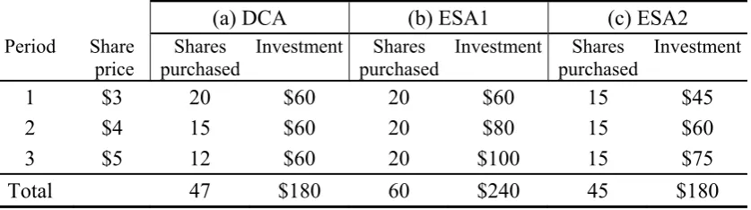
Table 2 shows the same strategies, but with the share price rising rather than falling.

The DCA strategy again invests $60 each period, but as prices rise fewer shares are

purchased in the later periods. Once again DCA achieves an average cost ($180/47=$3.83)

below the average price ($4) by buying more shares when they are relatively cheap. This

effectively compares the DCA strategy with the ESA2 strategy, which invests the same total

Table 2: Illustrative Comparison of Strategies as Share Prices Rise

DCA invests a fixed $60 per period, compared to buying Equal Share Amounts (ESA) of (b) 20 shares and (c) 15 shares per period. Rising prices mean that ESA1 invests a larger dollar total than DCA. ESA2 is the only ESA strategy which invests the same amount as DCA, but choosing the right number of shares in period one requires knowledge of future share prices.

(a) DCA (b) ESA1 (c) ESA2

Period Share

price

Shares purchased

Investment Shares

purchased

Investment Shares

purchased

Investment

1 $3 20 $60 20 $60 15 $45 2 $4 15 $60 20 $80 15 $60 3 $5 12 $60 20 $100 15 $75

Total 47 $180 60 $240 45 $180

However, as we saw earlier, the real alternative to DCA is ESA1. In practice our best

guess would again be to invest one third of our total budget in the first period, since if prices

were to stay at this level we would invest the correct amount. But when prices subsequently

rise we end up spending substantially more than this ($240). ESA2 invests the correct

amount, but it achieves this only by knowing that prices are about to rise and responding to

this knowledge by buying fewer shares than ESA1. Again, profits are reduced.

Comparing DCA’s average cost with the average price effectively compares DCA with

a strategy which uses perfect foresight in a way which systematically reduces profits and

increases losses. DCA’s proponents almost invariably refer to its lower unit costs, so this

cognitive error appears to be a key factor explaining the strategy’s continued popularity.

4. The Arithmetic of the Cognitive Error

This section demonstrates more formally that it is only by making a misleading comparison

that DCA appears to offer superior profits. We consider investing in an asset over a series of

n discrete periods. The price of the asset in each period i is pi. The alternative investment

profits at a subsequent point, after all investments have been made. If prices are then pT, the

profit made by the strategy is:





i pq

q pT

1 1

(1)

We define DCA as a strategy which invests b dollars in each period (piqi=b). This

gives us the profits that will result from following a DCA strategy:

nb

p

b

p

dca









We assume that investors who use DCA do not believe that they can forecast market

prices. In effect they assume that prices follow a random walk. As Brennan et al. (2005)

shows, mean reversion could under some limited circumstances lead DCA to outperform, but

the case that is normally made for DCA makes no claim that it is exploiting market

inefficiency − instead it is portrayed as a strategy which will outperform in any market.

Furthermore, DCA commits investors to invest the same amount no matter what price

movements they expect in the coming period. Those who (rightly or wrongly) believe that

they can forecast short-term price movements are likely to reject DCA and follow other

strategies instead.

We also assume that this random walk has zero drift.2 This assumption is generous to

DCA, since upward drift will tend to penalize the strategy for investing gradually. Investors

2 _{The assumption of zero drift need not imply a loss of generality, since drift could be incorporated}

by defining prices not as absolute market prices, but as prices relative to a numeraire which appreciates at a rate which gives a fair return for the risks inherent in this asset (pi*=pi/(1+r)i, where r

reflects the cost of capital and an appropriate risk premium). We could then assume that pi* has zero

expected drift since investors who use DCA will not believe that they can forecast short-term relative returns for assets of equal risk (those who do would choose other strategies). The results derived here

risk-presumably believe that over the medium term their chosen securities will generate an

attractive return, but they must also believe that the return over the short term (while they are

using DCA to build up their position) is likely to be small. Investors who expect significant

returns over the short term would prefer to invest immediately in one lump sum rather than

delay their investments by following a DCA strategy. Given these assumptions, investors

will assume ex ante that prices will remain flat, with E[pT /pi]=1 for all i. Substituting this

into Equation 2, we see that the ex ante expected profit from the DCA strategy is zero.

Our alternative investment strategy is to buy equal numbers of shares in each period

(qi=a). Substituting this into Equation 1 gives us:



  

 n

i i

esa anpT a p

1

1 ₍₃₎

The ex ante expected profit from this ESA strategy is also zero (this can be seen by

substituting E[pi]=E[pT] for all i, as an equivalent expression of our driftless random walk).

Thus DCA does not give superior expected returns.

This is an intuitive result. We can regard the total return as a weighted average of the

returns made on the amounts invested in each period. ESA and DCA differ only in giving

different relative weights to these individual period returns. But if prices are believed to

follow a random walk with zero drift the expected return will be zero for each period and

varying the relative weight given to different periods’ returns cannot change the expected

aggregate return.3 By contrast, DCA’s popular supporters suggest that even when investors

have no belief that they can forecast market returns they can nevertheless expect to beat the

market by using DCA.

As we saw in the previous section, the total amount invested under ESA1 (api) is

likely to differ from the amount (nb) invested under DCA. But the comparison that is usually presented by proponents of DCA assumes that the two techniques invest equal total amounts.

Thus to duplicate the conventional “proof” of the benefits of DCA, we need to rescale the

number of shares bought under ESA1 by the fixed factor (nb/api), so that an exactly equal

amount is invested by the two strategies. This gives us the expected profits resulting from

strategy ESA2:                        _n i esa esa i p a nb 1 1

2 ₍₄₎

The use of foresight can be seen in the fact that the scaling factor depends on the

average share price throughout the investment horizon. Only if this is known at the outset

would we be able to buy the correct number of shares so that we end up spending exactly the

same amounts under ESA2 and DCA. Substituting from Equation 3:

                   















_







i n i i esa i T

p

a

nb

p

a

anp

2 ₍₅₎

3 _{Expected profits can be expressed as}

_

_

_

_

_

_

_

_





Tq pq

p

1 1

. Our assumption of a random walk

implies that future price movements (pT/pi) are always independent of past values of pi and qi, so this

can be re-written as

_

_{ }

_



_{ }



                    n i i i n i i i i q p q p p p T 1 1

. But the random walk has zero drift, so E[pT/pi]=1

nb

p

p

bn







Subtracting Equation (6) from Equation (2) we find:

                             











nbp

2 1 1 ₍₇₎

The term in brackets is non-negative for positive pi, and strictly positive if they are not

all equal. This follows directly from the arithmetic mean-harmonic mean inequality.4

This achieves our objective. The analysis above shows that the expected profits from a

DCA strategy are identical to those from our ESA1 strategy (both give zero expected

profits). By contrast, DCA gives higher expected profits than our ESA2 strategy which

scales the level of investment so as to spend exactly the same total amount as DCA.

However, ESA2 is not a feasible strategy, since it uses perfect foresight to invest in a

systematically loss-making fashion. It is only on this biased comparison (DCA vs ESA2)

that DCA appears to make greater returns, yet it is exactly this comparison which is

implicitly being made when it is noted that DCA buys at an average cost which is lower than

the average price.

This biased comparison suggests that DCA makes profits of (PT – average purchase

cost) per share whereas other strategies make (PT – average price). Thus DCA appears to

shift the whole distribution of possible profits upwards by the extent of the difference

between these averages. For most investment strategies reducing the average purchase cost

4 _{The arithmetic-harmonic mean inequality is usually stated as: ( ... )/ /(1 ... 1 )}

1

1 xn n n _{x xn}

x     

for positive xi, so we have substituted

x



/

inequality that for any convex function f(.), using the function f(x) = 1/x (pi and qi

are positive for all i since DCA is a strategy for investing positive sums at positive prices).





[ ( )] [ ]

really will increase expected returns, so cost minimization is normally a useful heuristic goal

for investors. However, DCA reduces its average cost by increasing its purchases of shares

after prices have risen (and vice versa). This is a retrospective response to previous price

movements, and will boost expected profits only if asset prices systematically tend to

mean-revert. Comparing DCA’s average cost with the average market price is systematically

misleading since it implicitly compares DCA with a strategy where the amount invested

depends on foreknowledge of future prices. The error involved in this comparison has not

previously been identified5. Faced with such apparently obvious benefits, it should perhaps

not be surprising that DCA remains so popular.

5. The Sub-Optimality of DCA

A number of previous studies have attempted to explain DCA’s popularity by hypothesizing

that although inefficient in mean-variance terms, DCA could still be attractive to rational

investors whose risk preferences take alternative (non-variance) forms. This section shows

that this is an unproductive line of research, since DCA is a sub-optimal strategy regardless

of the investor’s risk preferences. For this purpose we use Dybvig’s Payoff Distribution

Pricing Model (Dybvig, 1988a and 1988b).

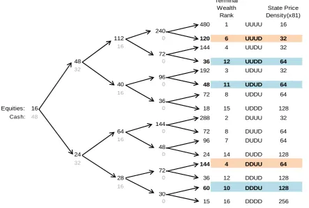
As a very simple illustration, Figure 1 shows a binomial model of a DCA strategy over

four periods. The equity element of the portfolio is assumed to double in a good outturn and

5 _{Thorley (1994) rightly argues that DCA is based on a fallacy, but does not correctly identify the}

halve in a bad outturn. At the start of the first period 16 is invested in equities, with 48 in

cash6. A further 16 of this cash is invested each period. All paths are assumed to be equally

likely. The key to this technique is comparing the terminal wealths with their corresponding

state price densities (the state price divided by the probability – in this case 16(1/3)u(2/3)d,

where u and d are the number of up and down states in the path concerned7). An efficient strategy will generate the highest terminal wealths in the paths for which these outturns are

“cheapest” (i.e. have the lowest state prices). This is generally the case in Figure 1, but there

are exceptions. DDUU results in a larger terminal wealth than UUUD despite seeing fewer

lucky outturns. Similarly, DDDU beats UUDD and UDUD. This can be loosely interpreted

as DCA making ineffective use of some comparatively lucky paths.

6 _{Investors with regular monthly income and expenditure streams may choose to save a fixed dollar}

amount each month, leaving them following a DCA strategy by default. However, proponents of DCA are not simply arguing that regular saving is desirable – they claim that it is advantageous to invest any available lump sum gradually rather than immediately. Thus we compare DCA with alternative ways of investing a lump sum.

7 _{More generally, the state price densities of one period up and down states are}

 

1 1rt

















compounded annual risk-free interest rate and the risky asset has annual expected return μ and

standard deviation σ. The corresponding one period risky asset returns are





Figure 1: Simple Model of DCA Strategy

This tree shows the value of the investor’s equity and cash holdings at the start of each period. Equity values double in a good outturn and halve in a bad outturn (for simplicity cash is assumed to earn no interest and any dividends are assumed immediately reinvested to give the total equity returns shown). Investors start with 16 invested in equities (the upper figure at each node) and 48 in cash (the lower figure). They then invest a further 16 in each subsequent period, leaving zero at the start and end of the final period. All paths are assumed to have equal real world probabilities (the corresponding risk neutral probabilities are 1/3 and 2/3). The sub-optimality of this strategy stems from the fact that in some cases (highlighted) paths with a higher state price density achieve higher terminal wealth than luckier paths with a lower state price density.

Terminal Wealth

Rank

State Price Density(x81)

480 1 UUUU 16

240

112 0 120 6 UUUD 32

16 _{144 4 UUDU 32}

72

48 0 36 12 UUDD 64

32 _{192 3 UDUU 32}

96

40 0 48 11 UDUD 64

16 _{72 8 UDDU 64}

36

Equities: 16 0 18 15 UDDD 128

Cash: 48 _{288 2 DUUU 32}

144

64 0 72 8 DUUD 64

16 _{96 7 DUDU 64}

48

24 0 24 14 DUDD 128

32 _{144 4 DDUU 64}

72

28 0 36 12 DDUD 128

16 _{60 10 DDDU 128}

30

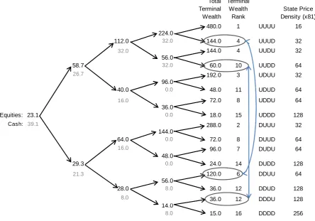
The inefficiency of DCA in this case can be demonstrated by deriving an alternative

strategy which generates exactly the same 16 outturns at lower cost. This is done by

changing our strategy to ensure that the best outturns occur in the paths which have the

lowest state price densities (i.e. the greatest number of up states), so we switch the outturns

for DDUU and UUUD in Figure 1, and those for DDDU and UUDD. The state prices can

then be used to determine the value of earlier nodes (thus determining the proportion of the

portfolio which must be held in cash at each point in order to duplicate the terminal wealth

outturns of a DCA strategy). This in turn determines the initial capital required to generate

these outturns. This alternative strategy is shown in Figure 2 and requires only 62.2 initial

capital (23.1 in equities and 39.1 in cash), compared to 64 above. This improvement is

achieved without additional borrowing, merely by making better use of existing capital. This

shows the degree to which DCA is inefficient. A key advantage of this method is that it

demonstrates DCA’s inefficiency without needing to specify the investor’s risk preferences,

since our alternative strategy generates exactly the same terminal wealth outturns as DCA at

a lower initial cost.8

8_{Earning an identical set of terminal wealth outturns at a lower initial cost (or, equivalently, greater}

Figure 2: Optimized Strategy Giving Identical Outturns to DCA

This tree shows the amounts invested in equities and in cash in each period with amount of cash held at the start of each period set to duplicate the outturns in Figure 1, but optimized so that the largest outturns occur in the paths with the lowest state price density (compared with Figure 1, the outturns for UUUD and DDUU have been switched, and the outturns for UUDD and DDDU). Returns on cash and equities are assumed the same as in Figure 1. The lower total capital (62.2) required by this optimized strategy shows the extent to which DCA is an inefficient strategy.

The amount of cash which must be held at each point is shown below the equity

holdings. We can see that the optimized strategy holds considerably less cash than DCA

during the first two periods. This supports the interpretation put forward by Rozeff (1994)

that DCA is inefficient because it takes too little exposure in the early periods, leaving

terminal wealth disproportionately sensitive to returns in later periods.

However, for volatility levels typical of developed equity markets this halving or

doubling of equity values at each step of the tree would represent a number of years between

each investment. We use this unrealistic assumption merely to allow us to show the

dynamic inefficiency in a very simple tree. For more plausible strategies we can consider 12

Total Terminal Wealth Terminal Wealth Rank State Price Density (x81)

480.0 1 UUUU 16

224.0

112.0 32.0 144.0 4 UUUD 32

32.0 144.0 4 UUDU 32

56.0

58.7 32.0 60.0 10 UUDD 64

26.7 _{192.0 3 UDUU 32}

96.0

40.0 0.0 48.0 11 UDUD 64

16.0 72.0 8 UDDU 64

36.0

Equities: 23.1 0.0 18.0 15 UDDD 128

Cash: 39.1 _{288.0 2 DUUU 32}

144.0

64.0 0.0 72.0 8 DUUD 64

16.0 _{96.0 7 DUDU 64}

48.0

29.3 0.0 24.0 14 DUDD 128

21.3 120.0 6 DDUU 64

56.0

28.0 8.0 36.0 12 DDUD 128

8.0 _{36.0 12 DDDU 128}

14.0

step trees corresponding to a DCA strategy of equal monthly investments over a one year

horizon. Such trees contains 4,096 outturns, and so are not shown here in full, but Table 3

shows that a wide range of different assumptions for the market risk premium and volatility

all result in efficiency losses. Furthermore, these losses are roughly proportional to the

assumed risk premium, which again supports the interpretation that they stem from the

returns foregone by holding excessive cash during the early periods. As a robustness check,

these calculations were replicated for an 18-step binomial tree, giving 262,144 outturns (the

maximum which was computationally practical). The resulting inefficiency estimates were

very similar to those in Table 2.3, being larger by a maximum of 0.01%.

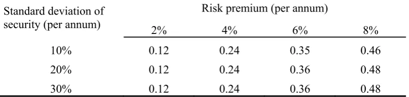
Table 3: Quantifying the Inefficiency of DCA (% of Initial Capital)

This table uses Dybvig’s PDPM model to derive the cost of an optimized strategy which generates the same set of final portfolio values as those achieved by a DCA strategy which invests one twelfth of its initial capital at the start of each month. The table shows the percentage by which the capital required by the DCA strategy is greater than that required by the optimized strategy to generate an identical set of outturns. These figures were derived using a 12 period binomial tree where returns are assumed IID with the binomial steps calibrated to give monthly returns distributed with the annualized risk premia and volatilities shown (almost identical results were found for a 18-step tree with 262,144 outturns). The risk-free rate is assumed to be 5%, but the results are not sensitive to this assumption (adjusting it to 0% or 10% alters these figures by less than 0.005%).

Standard deviation of Risk premium (per annum)

security (per annum) _{2% 4% 6% 8%}

10% 0.12 0.24 0.35 0.46

20% 0.12 0.24 0.36 0.48

30% 0.12 0.24 0.36 0.48

We have assumed that market returns have a binomial distribution, but the fact that the

level of volatility in Table 3 has very little effect on the size of the inefficiency is a

reassuring indication that these results are not sensitive to the particular distribution which is

assumed. More importantly, Rieger (2011) demonstrates formally that this inefficiency is not

specific to the binomial distribution ─ he generalizes Dybvig’s results, showing that

case) a non-monotonic relationship with market returns are sub-optimal regardless of the

distribution of market returns.

Taking the most plausible estimates of the risk premium to be around the middle of the

range shown in Table 3, the associated efficiency losses are modest, but should nevertheless

be regarded as economically significant. For example, sustained return differentials on this

scale are likely to be seen as relevant by investors when assessing the performance of

competing fund managers. Furthermore, these figures should be regarded as conservative

estimates of the actual efficiency losses. In each case the optimized strategy generates the

same outturns as DCA but uses less capital. This shows that DCA is inefficient regardless of

the form taken by investor risk preferences. This is a powerful result, but there is no reason

why in practice investors’ preferred option should be to replicate DCA’s outturns. Given

each investor’s specific preferences there are likely to be other strategies which are even

more attractive alternatives, so the efficiency losses shown in Table 3 must be regarded as

lower bounds.

In conclusion: DCA is an inefficient strategy for investing available funds, and this

result applies for all plausible forms of investor risk preference. Thus investors’ use of DCA

cannot be explained as a rational consequence of non-variance risk preferences. The

following section considers more plausible explanations for DCA’s popularity within

6. Behavioral Finance Effects

A number of papers have attempted to use standard finance theory to explain why investors

might rationally choose DCA despite its mean-variance inefficiency. These explanations

have not proved satisfactory. The previous section showed that explanations based on

non-variance investor risk preferences must be rejected and, as described above, other

explanations require unjustified assumptions about investors’ forecasts of asset returns. This

section instead considers explanations within behavioral finance. Specifically, Statman

(1995) sets out four behavioral finance effects which could help explain DCA’s popularity:

(i) Prospect theory and framing effects, (ii) Cognitive error, (iii) Aversion to regret and (iv)

Self-control problems. We consider each of these in turn.

Prospect theory has been rejected as an explanation of DCA’s popularity by

subsequent empirical studies and section 5 above demonstrates more generally that DCA is a

sub-optimal strategy regardless of the form taken by investor risk preferences. However,

Statman also suggests that DCA is attractive because it frames investment outturns in a

flattering manner, allowing investors to feel that they have already gained by buying at a

lower average cost. The cognitive error identified makes this framing effect more explicit,

and shows exactly why comparing DCA’s average cost with the average price is misleading:

Investors who frame their choice in terms of this comparison are making a specific

mathematical error. However, even though this error leads investors to choose a strategy

which is demonstrably (and measurably) inefficient in terms of the terminal wealth outturns

it generates, Statman notes that the psychological feelings of wellbeing that this misleading

framing creates could in principle offset the direct inefficiency costs of DCA.

Statman’s other points are based on indirect benefits to investors resulting from the

rigid investment timetable that DCA imposes. First, he identifies another form of cognitive

boost returns. There is plenty of evidence that investors’ market timing has tended to be poor

(e.g. Ritter 1991; Loughran and Ritter 1995), so DCA can indirectly increase expected

returns by preventing investors from trying to time the market. However, Hayley (2014)

shows that for the average US equity investor the effect of this bad timing is much smaller

than has been suggested by other recent studies, and smaller than the estimated efficiency

losses shown in Table 3. Investors with particularly bad timing may still find that the

benefits of not trying to time the market outweigh the inefficiencies of DCA, but this does

not appear to be the case for the average investor. Statman also notes that the discipline

imposed by DCA (i) prevents a myopic desire for greater current consumption from

interfering with investors’ long-term investment goals; (ii) reduces the feelings of regret

resulting from adverse market outcomes since investors feel less responsibility when DCA

restricts their choices. The strength of these explanations is that the existence of these

behavioral finance effects has been well established in other contexts. This comes in stark

contrast to the additional assumptions required by some rationalist explanations for DCA’s

popularity.

A normative case for using DCA can thus be constructed by weighing the inherent

inefficiency of DCA against the combined welfare costs of the investor regret, myopia and

bad timing associated with less disciplined investment strategies. However, the current

ill-informed analysis in the media gives little reason to suppose that such sensible reasoning is

often what leads investors to choose DCA. Instead DCA is generally recommended by its

proponents to all investors, with no reference to their specific preferences, objectives or

beliefs. Avoidance of regret is sometimes mentioned, but by far the most common rationale

given for DCA is that it boosts returns by buying at an average cost which is lower than the

Identifying the cognitive error in this argument thus gives a more straightforward

explanation for why many investors still choose DCA.

Identifying this cognitive error also brings very different welfare implications.

Previous research has argued that DCA could be welfare-improving (and hence an entirely

rational choice) for investors with specific types of non-variance risk preferences. The

analysis above rejects this argument. The wider behavioral finance benefits identified by

Statman (1995) suggest that use of DCA may nevertheless be beneficial, and in the absence

of convincing alternative explanations, it would be reasonable to presume that these effects

must be dominant in order to explain DCA’s continued popularity. By contrast, identifying

the cognitive error in the key argument used by DCA’s proponents opens up the possibility

that in failing to spot this error investors who use DCA may actually be reducing their

Conclusion

DCA has long been shown to be mean-variance inefficient, so recent research has focused on

explaining why it nevertheless remains so popular. Recent papers have attempted to derive

entirely rational explanations for DCA’s popularity, but these are not satisfactory.

Specifically, this paper demonstrates that DCA is a sub-optimal strategy regardless of

investor risk preferences, so explanations based on alternative forms of such preferences

must be rejected.

The other contribution made by this paper is to explicitly identify the error involved in

comparing DCA’s average purchase cost with the average market price. DCA’s popularity

can now be regarded as resulting from a specific and demonstrable cognitive error. This

gives us a better explanation of DCA’s popularity since – unlike most other explanations – it

addresses the argument that is normally central to the case made by proponents of DCA.

DCA’s demonstrable inefficiency could be outweighed by its wider behavioral benefits

(less regret and reduced impact from investor myopia and inappropriate attempts to time the

market). If DCA were recommended to investors on the basis of such psychological benefits

then we might be confident that on balance it is welfare-improving, but the fact that it is

generally recommended to investors on the basis of a flawed argument related to its lower

References

Brennan, M. J., F. Li, and W.N. Torous, 2005. Dollar cost averaging. Review of Finance 9, 509-535.

Constantinides, G. M., 1979. A note on the suboptimality of dollar-cost averaging as an investment policy. Journal of Financial and Quantitative Analysis14 443-450.

Dichtl, H., and W. Drobetz, 2011. Dollar-cost averaging and prospect theory investors: an explanation for a popular investment strategy. The Journal of Behavioral Finance12 41-52.

Dubil, R., 2005. Lifetime dollar-cost averaging: forget cost savings, think risk reduction. Journal of Financial Planning18 86-90.

Dybvig, P.H., 1988a. Inefficient dynamic portfolio strategies or how to throw away a million dollars in the stock market. The Review of Financial Studies 1 67-88.

Dybvig, P. H., 1988b. Distributional analysis of portfolio choice. Journal of Business, 369-393.

Greenhut, J. G., 2006. Mathematical illusion: why dollar-cost averaging does not work. Journal of

Financial Planning19 76-83.

Hayley, S., 2014. Hindsight effects in dollar-weighted returns. Journal of Financial and Quantitative Analysis, 49(1) 249 – 269.

Knight, J. R., and L. Mandell, 1992/93. Nobody gains from dollar cost averaging: analytical, numerical and empirical results. Financial Services Review2 51-61.

Fruhwirth, M., and G. Mikula, 2008. Can prospect theory explain the popularity of savings plans? Working paper, available at SSRN: http://ssrn.com/abstract=1681343.

Leggio, K., and D. Lien, 2001. Does loss aversion explain dollar-cost averaging? Financial Services

Review 10 117-127.

Leggio, K., and D. Lien, 2003. Comparing alternative investment strategies using risk-adjusted

performance measures. Journal of Financial Planning 16 82-86.

Milevsky, M. A., and S.E. Posner, 2003. A continuous-time re-examination of the inefficiency of dollar-cost averaging. International Journal of Theoretical & Applied Finance6 173-194.

Rieger, M. O., 2011. Co-monotonicity of optimal investments and the design of structured financial products. Finance and Stochastics15 27-55.

Ritter, J., 1991. The long-run performance of initial public offerings. Journal of Finance46 3-27.

Rozeff, M. S., 1994. Lump-sum investing versus dollar-averaging. Journal of Portfolio Management

20 45-50.

Statman, M., 1995. A behavioral framework for dollar-cost averaging. Journal of Portfolio

Management22 70-78.

Thorley, S. R., 1994. The fallacy of dollar cost averaging. Financial Practice and Education 4

138-143.

Trainor, William J Jr., 2005. Within-horizon exposure to loss for dollar cost averaging and lump sum investing. Financial Services Review14 319-330.

Williams, R. E. and P.W. Bacon, 1993. Lump-sum beats dollar cost averaging. Journal of Financial