City, University of London Institutional Repository
Citation
:
Faria, C. F. D. M. and Fring, A. (2007). Non-Hermitian Hamiltonians with real
eigenvalues coupled to electric fields: From the time-independent to the time-dependent
quantum mechanical formulation. Laser Physics, 17(4), pp. 424-437. doi:
10.1134/S1054660X07040196
This is the unspecified version of the paper.
This version of the publication may differ from the final published
version.
Permanent repository link:
http://openaccess.city.ac.uk/696/
Link to published version
:
http://dx.doi.org/10.1134/S1054660X07040196
Copyright and reuse:
City Research Online aims to make research
outputs of City, University of London available to a wider audience.
Copyright and Moral Rights remain with the author(s) and/or copyright
holders. URLs from City Research Online may be freely distributed and
linked to.
City Research Online:
http://openaccess.city.ac.uk/
[email protected]
arXiv:quant-ph/0609096v2 15 Jan 2007
from the time-independent to the time dependent quantum mechanical formulation
C. Figueira de Morisson Faria and A. Fring
Centre for Mathematical Science, City University, Northampton Square, London EC1V 0HB, UK
We provide a reviewlike introduction into the quantum mechanical formalism related to non-Hermitian Hamiltonian systems with real eigenvalues. Starting with the time-independent frame-work we explain how to determine an appropriate domain of a non-Hermitian Hamiltonian and pay particular attention to the role played byPT-symmetry and pseudo-Hermiticity. We discuss the time-evolution of such systems having in particular the question in mind of how to couple consis-tently an electric field to pseudo-Hermitian Hamiltonians. We illustrate the general formalism with three explicit examples: i) the generalized Swanson Hamiltonians, which constitute non-Hermitian extensions of anharmonic oscillators, ii) the spiked harmonic oscillator, which exhibits explicit super-symmetry and iii) the−x4-potential, which serves as a toy model for the quantum field theoretical
φ4
-theory.
I. INTRODUCTION
In general most physicists will almost instinctively associate a non-Hermitian Hamiltonian with unstable states, decaying wavefunctions, resonances and dissipa-tion. Such type of systems have been studied for a long time. They arise for instance when coupling channels in a system in which the wavefunctions factorize into func-tions which depend on separate sets of variables. The effective Hamiltonians resulting in this manner are non-Hermitian and have complex eigenvalues [1]. However, one should note that Hermiticity of the Hamiltonian is only a sufficient condition, which guarantees real eigen-values and the conservation of probability densities. It needs to be emphasized that it is not a necessary con-dition and there could be non-Hermitian Hamiltonians withreal discrete eigenvalue spectra, which then consti-tute potential candidates for physical applications, such as for instance atomic systems without decay.
Precisely such type of Hamiltonian systems are cur-rently under intense investigation (for a collection of re-cent results see for instance [2]). The re-central question in this context is of course how to obtain a consistent quantum mechanical framework. So far much effort has gone into the study of time-independent eigenvalue prob-lems. The main question we wish to address here is how to couple an external time-dependent electric field to a non-Hermitian Hamiltonian with real eigenvalues [3].
Our manuscript is organized as follows: For the bene-fit of the non-expert and the audience of this conference we commence in section II with a brief reviewlike intro-duction by recalling some by now well-known facts and arguments on the consistent quantum mechanical formu-lation of non-Hermitian Hamiltonian systems. In section A we review the time-independent formulation starting with a discussion of how to determine the appropriate do-main for a non-Hermitian Hamiltonian from the choice of asymptotic boundary condition. In part 2 of this section we explain the limited role played by PT-symmetry. In part 3 of section A we explain how pseudo-Hermiticity can be employed to map almost all relevant problems in
the non-Hermitian scenario to a Hermitian system in the same equivalence class. The two systems obtained in this manner are therefore isospectral. In section B we discuss how this formalism can be extended to include an evo-lution in time. We describe here gauge transformations, perturbation theory and how to compute various phys-ical quantities in the non-Hermitian setting. In section III we discuss two methods of how to solve one of the key problems in this context, namely how to compute pseudo-Hermitian Hamiltonians. Section IV contains three ex-plicit examples to which the formulation from the previ-ous sections applies: i) the generalized Swanson Hamilto-nians, which constitute non-Hermitian extensions of an-harmonic oscillators, ii) the spiked an-harmonic oscillator, which exhibits explicit supersymmetry and iii) the−x4
-potential, which serves as a toy model for the quantum field theoreticalφ4-theory. We state our conclusions and
an outlook to further problems in section V.
II. THE GENERAL FRAMEWORK
A. Time-independent quantum mechanical formulation
1. The domain of non-Hermitian Hamiltonians
The current interest in this subject was triggered eight years ago [4] by the at the time rather surprising numer-ical observation that the Hamiltonian
H=p2−g(iz)N (1)
defined on a suitable domain possesses a real positive and discrete eigenvalue spectrum for integers N ≥ 2 with positive real coupling constant g. This property holds despite it being non-HermitianH 6=H† and unbounded
from below, for N = 4n with n∈ N. Throughout this paper we use atomic units~=e=me=cα= 1.
select a meaningful domain. In [4] it was argued that the natural boundary condition, Φ(z)→0 exponentially
for |z| → ∞, requires that one continues the eigenvalue
problem into the complexz-plane. In fact, forH in (1) it was found that the wedges bounded by the Stokes lines in which this boundary condition holds are given by
WL(N) =
θ
−
8 +N
2(N+ 2)π < θ <− 4 +N
2(N+ 2)π
, (2)
WR(N) =
θ
−
N
2(N+ 2)π < θ <
4−N
2(N+ 2)π
, (3)
where θ = argz. To see this one can follow the proce-dure for an asymptotic expansion of a differential oper-ator as outlined for instance in [5]. Substituting Φ(z) = exp(ϕ(z)) into the eigenvalue equationHΦ =εΦ yields
ϕ′′+ (ϕ′)2+g(iz)N +ε= 0. For|z| → ∞ with infinity
being an irregular singular point one may assume that
ϕ′′≪(ϕ′)2. For largezwe can also neglectεin
compar-ison with the potential and obtain
ϕ(z)∼ 2
√g
N+ 2i
(1+N
2)z(1+
N
2) for |z| → ∞. (4)
In order to extract the dominating exponential factor in Φ(z) and to achieve Φ(z) →0 for |z| → ∞, we require Reϕ(z)<0. Withθ= argzthis is equivalent to
sin
πN
4 + 2 +N
2 θ
>0, (5)
which amounts to the conditions (2), (3) for the left and the right wedge WL and WR, respectively. Of course
(5) allows for many more solutions and therefore possi-ble wedges, but the selection criterion for (2), (3) is to reproduce the conventional wedge for the harmonic oscil-lator forN= 2, which is centered around the real axis.
This means the domain of integration, which makes the eigenvalue problem of the non-Hermitian Hamilto-nian operator in (1) in position space well defined for the asymptotic boundary condition Φ(z)→0 exponentially
for|z| → ∞is any path in the complexz-plane which
re-mains inside the wedgesWLandWRwhen it approaches
complex infinity. This means any path parameterized as
z(x) withx∈R, which satisfies lim
x→±∞arg[z(x)]∈ WR/L (6)
guarantees the appropriate boundary condition, namely exponential decay at infinity of the wavefunction Φ(z). For various purposes, for instance when one is concerned about a fast numerical convergence, one can also deter-mine the anti-Stokes lines, that is the domain on which the wavefunction vanishes most rapidly, see e.g. [5]. For
Hin (1) the anti-Stokes anglesθAS
L/Rare just in the centre
ofWL andWR [4].
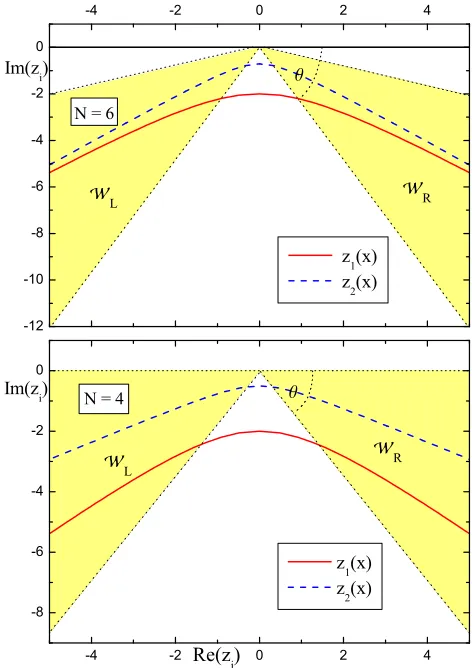
Permissible domains are therefore usually some form of parameterizations for hyperbolae. For instance a modi-fied version of a parameterization used in [6] was sug-gested in [7]
z1(x) =xcos(θASR ) +isin(θASR )
p
a2+x2 (7)
witha∈R. This clearly satisfied the required asymptotic lim
x→±∞arg[z1(x)] =θ AS
R/L(N)∈ WR/L(N). (8)
for all values ofN. However, as we shall discuss in more detail in section IV certain manipulations depend cru-cially on the suitable choice of the parameterization and one needs various alternatives. The selection procedure for what is most ”appropriate” is largely left to inspired guess work at this stage. As we shall see below, an ex-tremely useful variation of (7) was provided in [8]
z2(x) =−2i√1 +ix (9)
with
lim
x→∞arg[z2(x)] =− π
4 ∈ WR(N)
lim
x→−∞arg[z2(x)] = −3π
4 ∈ WL(N)
(10)
for N = 3,4, . . . ,9. Another permissible parameteriza-tion can be found for instance [9]. We illustrate the above discussion with some examples in figure 1:
-4 -2 0 2 4
-8 -6 -4 -2 0
R
L
N = 4 Im(z
i
)
Re(z
i
)
z
1
(x)
z
2
(x) -12
-10 -8 -6 -4 -2 0
-4 -2 0 2 4
z
1
(x)
z
2
(x)
L
R
N = 6 Im(z
i
[image:3.612.327.563.316.650.2])
Figure 1: Stoke wedges in which the eigenfunctions ofH in (1) forN= 4,6 vanish exponentially when|z| → ∞. Permis-sible pathsz1 with a=1 andz2 as parameterized in (7) and
2. PT-symmetry and real eigenvalues
So how can one explain such unconventional behaviour that a non-Hermitian Hamiltonian possesses a real eigen-value spectrum? Shortly after the above mentioned ob-servation it was suggested that the reality of the spec-trum should be attributed to unbroken PT-symmetry [10], that is the validity of thetworelations
[H,PT] = 0 and PTΦ = Φ, (11) where Φ is a square integrable eigenfunction on some domain ofH. In other words, when the Hamiltonianand
the wavefunction remain invariant under a simultaneous parity transformationP and time reversalT
P : p→ −p z→ −z
T : p→ −p z→z i→ −i
PT : p→p z→ −z i→ −i,
(12)
the eigenvalues of H are real. As an example one sees that obviously the Hamiltonian in equation (1) is PT -symmetric. What is less straightforward to see is that for N < 2 the second relation in (11) does not hold. Analytic arguments, which establish these facts for the Hamiltonian (1) may be found in [11, 12].
We shall now outline to what extend PT-symmetry can be utilized. Clearly P2 = T2 = (PT)2 = I and
the last relation in (12) implies that the PT-operator is an anti-linear operator, i.e. it acts as PT(λΦ +µΨ) =
λ∗PTΦ +µ∗PTΨ with λ, µ ∈ Cand Φ,Ψ being
eigen-functions of the Hamiltonian H with eigenenergies ε,
HΦ = εΦ. The anti-linear nature of the PT-operator serves well to establish the reality of the spectrum, i.e.ε=ε∗, whenboth relations in (11) hold. This follows
simply from
εΦ =HΦ =HPTΦ =PTHΦ =PTεΦ =ε∗PTΦ
=ε∗Φ. (13)
Unfortunately, the anti-linearity is also responsible for the possibility that only the first identity in (11) could hold, but not the second. In this situation one speaks of a brokenPT-symmetry. The argument leading to this is straightforward [13, 14]: Let us consider first a unitary operatorU for which by definition
hUΨ|UΦi=hΨ|Φi (14)
holds for all eigenfunctions Φ,Ψ of H. From equation (14) it follows thatUΨ =uΨ with|u|= 1 for all Ψ, which means that a unitary operator has only one dimensional representations. This property changes for anti-unitary operatorsA, as in that case onlyA2is a unitary operator,
which can be seen from
A2Ψ
A2Φ
=hAΦ|AΨi=hΨ|Φi. (15) Now we can only deduce from (15) thatA2Ψ =a2Ψ with
a2
= 1 for all Ψ and this means that an anti-unitary
(which is implied by anti-linearity) operator could have a two dimensional representationAΨ =a∗Φ, AΦ =aΨ.
Indeed whenais purely imaginary one can not construct a linear combination Ω =λΦ +µΨ,withλ, µ∈Cof the two so-called flipping states Φ,Ψ, which remains invari-ant under the action ofA. We see that
AΩ =λ∗aΨ +µ∗a∗Φ =λΦ +µΨ (16)
implies that µ =λ∗a, λ= µ∗a∗ and therefore a2 = 1.
This means that only for a = ±1 the two-dimensional representation is reducible and for purely complex a it is irreducible. In the latter situation the second relation in (11) does therefore not hold. From (13) we see that
PTΦ is an eigenfunction of H with eigenvalueε∗ when
Φ is an eigenfunction ofH with eigenvalueε. Thus when the second relation in (11) does not hold the eigenvalues ofH come in complex conjugate pairs.
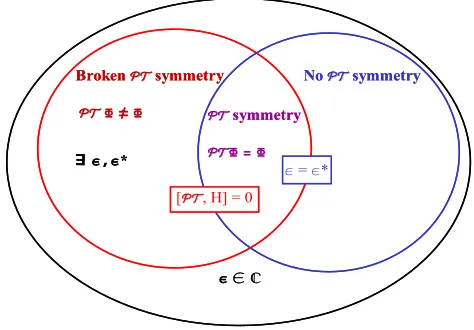
Thus PT-symmetry is merely a fairly good guiding principle and serves to identify immediately potentially interesting non-Hermitian Hamiltonian systems. How-ever, as argued above the PT-symmetry of H does not constitute a guarantee for a real eigenvalue spectrum. It remains an open question at this stage to determine under which circumstances thePT-symmetry is broken, albeit for Hamiltonians acting in a finite dimensional Hilbert space an algorithm based on stability theory has been provided [15]. In addition one should stress, that
PT-symmetry can not be regarded as the fundamental property, which explains always the reality of the spec-trum for non-Hermitian Hamiltonian systems as there ex-ist also examples with real spectra for which not even the Hamiltonian isPT-symmetric [3, 16] (see also examples below). In fact, more fundamental is the necessary and sufficient condition that the Hamiltonian must be Hermi-tian with regard tosome positive definite inner product [17] as we shall discuss next.
We summarize the role played byPT-symmetry in fig-ure 2:
No s ymmetry
B roken s ymmetr y
s ymmetry
*
E
= *
[ , H] = 0
No s ymmetry
B roken s ymmetr y
s ymmetry
*
E
= *
[image:4.612.326.563.531.696.2][ , H] = 0
3. Pseudo-Hermiticity and real eigenvalues
The formal question of how to establish a consis-tent quantum mechanical formalism for non-Hermitian Hamiltonian systems has already been discussed in [18] prior to the above mentioned numerical observation. In fact the possibility of extending a Hilbert space by a new intermediate state, which then leads to an indefinite met-ric has already preoccupied particle physicists more than half a century ago [19]. Some of these old results have recently been re-discovered and developed further. As already mentioned Hermiticity is a useful property as it guarantees the reality of the spectrum. Let us briefly re-call this standard argument and discuss how it needs to be altered for the present scenario.
Suppose we have a diagonalizable Hermitian (symmet-ric) operator h with regard to the conventional inner product
hφn|hφmi=hhφn|φmi. (17)
We use here Hermiticity in the sense that it implies self-adjointness and ignore possible subtleties, which might arise from domain issues. In general we understand here the domain to be the entire real axis. Multiplying next the eigenvalue equations
|hφmi=εm|φmi and hhφn|=ε∗nhφn|. (18)
byhφn|and|φmi, respectively, we obtain
hφn|hφmi=εmhφn|φmi (19)
hhφn|φmi=εn∗hφn|φmi. (20)
Taking the difference between (19) and (20) thus implies forn=mthat Hermiticity ofhwith regard to the stan-dard positive-definite inner producthφn|φmi, i.e. the
va-lidity of (17), is a sufficient condition for the energiesεn
to be real. Taking next n 6= m Hermiticity then also implies the orthogonality of the states|φnifor alln.
It turns out that for non-Hermitian operators we only need to change the definition for the inner prod-uct, i.e. change the metric, to draw the same conclu-sions [17, 18]. Taking now the domains as discussed in section 3, by definition we obviously no longer have
hΦn|HΦmi = hHΦn|Φmi for a non-Hermitian operator
H with Φnobeying the eigenvalue equation
H|Φni=εn|Φni. (21)
Therefore there is no guarantee for the reality of the spec-trum and neither for the orthogonality. However, assum-ing η to be a Hermitian operator with respect to the standard inner product, we can define a new inner prod-uct
hΦn|Φmiη:=hΦnη2Φm. (22)
Supposing now that H is Hermitian with regard to this new inner product
hΦn|HΦmiη=hHΦn|Φmiη, (23)
we may employ exactly the same arguments as above and ensure the reality of the spectrum as well as the orthogonalityhΦn|Φmiη =δn,m. Note that with regard
to the standard inner product one finds in general that
hΦn|Φmi 6=δn,m, see e.g. [10].
What is left is to characterize in more detail and possi-bly to determine is the metric operatorη2. Mostafazadeh
[17, 20, 21, 22] proposed to assume thatH is a pseudo-Hermitian operator satisfying
h=ηHη−1=h†=η−1H†η ⇔ H†=η2Hη−2, (24) where η is the Hermitian operator with regard to the standard inner product as introduced above. Since the Hermitian Hamiltonianhand the non-Hermitian Hamil-tonianH are related by a similarity transformation, they belong to the same similarity class and therefore have the same eigenvalues. The corresponding time-independent Schr¨odinger equations are then simply (18) and (21), where the corresponding wavefunctions are related as
Φ =η−1φ. (25)
Having real eigenvalues for the Hermitian Hamiltonian
hthen guarantees by construction the same real eigen-spectrum also forH. In fact the necessary and sufficient condition (23), which ensures the reality of the spectrum forH follows then from (17)
hΨ|HΦiη=hΨ
η2HΦ
= η−1ψ
η2Hη−1φ
=hψ
ηHη−1φ
=hψ|hφi=hhψ|φi=
ηHη−1ψ φi
=hHΨ|ηφi=hHΨ|η2Φ
=hHΨ|Φiη. (26)
Clearly, when η is Hermitian with regard to the stan-dard inner product it is also Hermitian with regard to theη-inner product (22).
A particular example for anη-inner product is the one introduced in [10]
hΨ|ΦiCPT := (CPT |Ψi)
T
· |Φi, (27)
where the new operatorC, withC2 =I, [H,C] = 0 and
[C,PT] = 0, is employed. In position space it reads
C(x, y) = P
nΦn(x)Φn(y). The operatorsC and η2 are
simply related asC=η−2P.
In addition one should stress that in fact these inner products can also be derived [23, 24] when starting from a biorthonormal basis, which is quite common to use in the study of non-Hermitian Hamiltonian systems with complex eigenvalues, that is decaying states, see e.g. [25, 26].
Crucial for a proper quantum mechanical framework is of course to clarify the nature of the physical observ-ables. In order to be suitable for a physical interpreta-tion, observablesO have to be Hermitian operators act-ing in some physical Hilbert space. From what has been outlined above with regard to the inner products, it is natural to take them to be Hermitian with respect to the newη-inner product
This implies immediately that whenois an observable in the Hermitian system, then
O=η−1oη ⇔ O=η−2O†η2 (29)
is an observable in the non-Hermitian system. This means in turn that the standard position operatorxand the momentum operators p are in general not observ-able in the Hermitian system, but rather their non-Hermitian counterparts X and P, respectively. Clearly
X andP satisfy the standard canonical commutation re-lations [X, P] =iwhen [x, p] =i. For Hamiltoniansh, H, which admit a polynomial expansion in {x, p}, {X, P}, it follows then directly from (24) that
H(x, p) =η−1h(x, p)η=h(X, P), (30)
h(x, p) =η−1H†(x, p)η=H†(X, P). (31)
These relations serve for instance as a consistency check when we start with a given non-Hermitian Hamiltonian and construct its Hermitian counterpart by means of a similarity transformation. Moreover (30) provides a sim-ple way to express the non-Hermitian Hamiltonian in terms of the canonical (X, P)-variables, which have a physical meaning for that system rather than the (x, p )-variables, which are in general meaningless in that con-text. In addition, one may use (30) as a principle to construct non-Hermitian Hamiltonians with real spectra from a given Hermitian Hamiltonian and a set of canon-ical variables and vice versa with (31). When η is PT -symmetric in the (x, p)-variables the corresponding quan-tities in the non-Hermitian system will bePT-symmetric in the (X, P)-variables.
We conclude with a final comment in regard to the uniqueness of the metric operator η2. In fact there are
various types of ambiguities arising, which we comment on in section III when we discuss how to computeη2
ex-plicitly. In [18] Scholtz, Geyer and Hahne proved that the metric operator η2 is uniquely determined on a Hilbert
space if and only if a set of observablesOiwith respect to
(28) is irreducible on this Hilbert space. The latter means that there is no bounded operator besides the identity, which commutes with all observables Oi. Taking this
result into account allows to move the nature of the am-biguities from the metric to the specification of the set of observables. As we shall see below a subset or even one observable might be enough in practise.
B. Time-dependent quantum mechanical formulation
Let us now discuss how to couple a laser field to the non-Hermitian Hamiltonians H, which have the proper-ties described above. In the simplest scenario, i.e. if the parameters involved lie within a non-relativistic regime and the dipole approximation holds, such a field can be approximated by a time-dependent electric fieldE(t). In the following, we will briefly recall our recent results on
the temporal evolution of the resulting system [3]. For simplicity, we assume thatE(t) is linearly polarized and has a finite durationτ.
Within a Hermitian framework and in the length gauge, such an evolution is described by the time-dependent Schr¨odinger equation
i∂tφ(t) =hl(t)φ(t), (32)
where
hl(t) =p
2
2 +V(x) +xE(t) =h+xE(t) (33)
is the Stark-LoSurdo Hamiltonian [27, 28]. For a pulse of finite duration,hφ(0) =εφ(0) andhφ(τ) =εφ(τ). We assume here thath possesses a non-Hermitian counter-partH which is in the same equivalence class, i.e. the validity of the first relation in (24).
1. Time-evolution operators
The central quantity of interest in this context is the time-evolution operator
u(t, t′) =Texp
−i
Z t
t′ dsh(s)
, (34)
which evolves a wavefunction from a time t′ to t, that
is φ(t) = u(t, t′)φ(t′). In (34), T denotes the time
or-dering. One should note that, in general, u(t, t′) 6=
exp [−ih(t−t′)]. In fact, such a relation only holds for
Hamiltonians which are not explicitly time-dependent, as is not the case for the scenario we have in mind.
Whenh(s) is a self-adjoint operator in some Hilbert space,u(t, t′) satisfies the relations [29, 30, 31]
i∂tu(t, t′) =h(t)u(t, t′),
u(t, t′)u(t′, t′′) =u(t, t′′) andu(t, t) =I. (35)
We will now assume that the similarity transformation
η extends to the time-dependent case. Thus, H(t) =
η−1h(t)η , with H(t) 6= H†(t). We take η to be
time-independent. This allows us to guarantee that the rela-tions
i∂tU(t, t′) =H(t)U(t, t′),
U(t, t′)U(t′, t′′) =U(t, t′′) andU(t, t) =I, (36)
for the time-evolution operatorU(t, t′) =η−1u(t, t′)η
as-sociated to the non-Hermitian Hamiltonian H(t), also hold. Then this operator fulfills the conditionU†(t, t′) =
η2U−1(t, t′)η−2,which follows from u†(t, t′) =u−1(t, t′).
guarantee that the time-dependent Schr¨odinger equation and the relations involving the time evolution operator remain valid also in the non-Hermitian case.
These conditions, however, are far more general than those normally encountered in the literature. In fact, most studies make several simplifying assumptions on the time-evolution operator, in the sense that they con-centrate on Hamiltonians which are either not explic-itly time-dependent, or which vary adiabatically and/or periodically with time. The first scenario is addressed by either solving the eigenvalue problem HΦ = εΦ,
or, at most, by employing the time-evolution operators
U(t, t′) = exp[−iH(t−t′)].
The remaining situations are widespread in the atomic physics literature, in the context of open quantum sys-tems. Roughly speaking, if a system is close to the adia-batic limit this means that it is varying so slowly that the problem can be reduced to solving eigenvalue equations of the formH(t)Φ(t) =εn(t)Φ(t). In a standard, Hermitian
framework, this implies that∂tu(t)u†(t)≪u(t)h(t)u†(t),
and that transitions between different time-dependent eigenstates of H(t) will be induced by perturbations around the adiabatic limit. Specifically for a system coupled to an external laser field, the time-dependent energies εn(t) give the field-dressed states (for a first
derivation of the adiabatic theorem and for an extension of such a theorem to non-Hermitian open quantum sys-tems, see [32] and [33], respectively). For periodic fields, such a procedure is closely related to the Floquet theory, for which there also exists time-dependent “quasiener-gies”. This approach may be problematic if the field varies abruptly with time, such as, for instance, if it is an ultrashort pulse.
2. Time-dependent physical quantities
The time-evolution operators characterized in the pre-vious subsection may then be employed to compute var-ious quantities of physical interest, such as for instance the transition probability
Pn←m=
hΦn|U(t,0) Φmiη 2
=|hφn|u(t,0)φmi|2, (37)
from an eigenstate |φmi to |φni of the Hermitian
elec-tric field-free Hamiltonian h or eigenstate |Φmi to |Φni
of the non-Hermitian electric field-free Hamiltonian H. Another physical quantity of interest is the time evolu-tion for the expectaevolu-tion value of an observable in the statenis
On(t) =hU(t,0)Φn(0)|OU(t,0)Φn(0)iη
=hu(t,0)φn(0)|ou(t,0)φn(0)iη (38)
=on(t).
In a similar way we may proceed to compute ionization rates and probabilities etc., but these examples are suf-ficient to see that, as in the time-independent scenario,
the relevant computations for the non-Hermitian system can be translated into the Hermitian one, provided the
η-operator is known.
3. Gauge transformations
Apart from employing the length-gauge Hamiltonian
hl(t), one may describe a Hermitian Hamiltonian system
coupled to an electric field in other gauges. Concrete examples are the velocity gauge, obtained by employing the minimal-coupling prescription p→ p−b(t), or the Kramers-Henneberger gauge, obtained with the shiftx→
x−c(t) in the field-free Hamiltonianhas introduced in (33). The corresponding Hamiltonians are given by
hv(t) = (p−b(t))
2
2 +V(x) =h(p−b(t)) (39) and
hKH(t) =
p2
2 +V(x−c(t)) =h(x−c(t)), (40) respectively. In equation (39) and (40),
b(t) =
Z t
0
dsE(s), c(t) =
Z t
0
dsb(s) (41)
are the momentum transferb(t) from the laser field to the system in question and the classical displacementc(t) in the system caused by the laser field.
Depending on the problem at hand, the gauge choice may considerably facilitate the computations. For in-stance, the length gauge is very appropriate for pertur-bation theory in the electric field, as the field coupling involves only one additional term, or for physical inter-pretations in the low-frequency regime, since it allows the physical picture of an effective time-dependent potential. The Kramers-Henneberger gauge is most useful in the high-frequency regime, especially if one wishes to exploit the periodicity of the field and perform Floquet expan-sions. Each formulation can be obtained from the other employing gauge transformations. The Hamiltonians in the length, velocity and Kramers-Henneberger gauge are related by
hl(p, x)−xE(t) =hv(p+b(t), x) =hKH(p, x+c(t)). (42)
We will now perform such transformations for non-Hermitian Hamiltonian systems. First, we will replace the wavefunction φ in the time-dependent Schr¨odinger equation related to the Hamiltonianhbyφ=a(t)−1φ′,
with a(t) being some unitary operator. This yields [29, 30, 31]
i∂tφ′=h′(t)φ′=a(t)h(t)a(t)−1+i∂ta(t)a(t)−1φ′. (43)
Kramers-Henneberger gauge, which are extensively used in strong-field laser physics, are given by,
al→v(t) =eib(t)x and av→KH(t) =eid(t)e−ic(t)p. (44)
respectively. In equation (44), in addition to the momen-tum transfer and classical displacement, we have also in-troduced the classical energy transferd(t) = 12Rt
0dsb(s) 2.
If the system is pseudo-Hermitian, one may employ the relationφ=ηΦ to obtain the gauge transformation
i∂tΦ′=A(t)H(t)A(t)−1+i∂tA(t)A(t)−1Φ′, (45)
where
a(t) =ηA(t)η−1 andh(t) =ηH(t)η−1, (46)
and the expression in brackets, on the right-hand-side of (45), denotes the gauge-transformed HamiltonianH′(t).
The gauge transformationsA(t), as it should be, guar-antee the invariance of the physical observables, when computed using the generalized inner product (22). Now the relations
Hl(X, P) =Hv(X, P+b(t)) +XE(t) (47)
=HKH(X+c(t), P) +XE(t),
hold for pseudo-Hermitian Hamiltonians.
4. Perturbation theory
Since, in most realistic situations, the time-dependent Schr¨odinger equation describing the evolution of a sys-tem with a binding potentialV(x) subjected to a time-dependent laser field E(t) does not possess an analytic solution, it is necessary to resort to perturbation theory. In order to construct a perturbative series in a pseudo-Hermitian framework, we will initially consider a time-dependent Hermitian Hamiltonianh(t) =h0(t) +hp(t),
where h0(t) and hp(t) are also Hermitian and satisfy
the time-dependent Schr¨odinger equation. Using the Du Hamel formula [29, 30, 31], we can express the time-evolution operatoru(t, t′) associated toh(t) as
u(t, t′) =u0(t, t′)−i
Z t
t′
u(t, s)hp(s)u0(s, t′)ds, (48)
where u0(t, t′) is the time evolution operator with
re-spect to h0(t). Equation (48) can then be solved itera-tively to an arbitrary order in hp(t), which will be the
perturbation. Roughly speaking if hp(t) ≪ h0(t), the
series obtained by such means has a great chance to con-verge. For instance, for weak laser fields and in the length gauge, a natural choice is to take hp(t) = xE(t) and
h0(t) =p2/2 +V, whereas in the strong-field regime we
takeh0(t) =p2/2 +xE(t) as the Gordon-Volkov Hamil-tonian and the perturbation is chosen ashp(t) =V.
Similarly, for the time evolution operator U(t, t′)
related to its pseudo-Hermitian counterpart H(t) =
H0(t) +Hp(t), with H0(t) = η−1h0(t)η and Hp(t) =
η−1h
p(t)η, we may also write
U(t, t′) =U0(t, t′)−i
Z t
t′
U(t, s)Hp(s)U0(s, t′)ds, (49)
whereU0(t, t′) is related to the HamiltonianH0(t), and
the perturbative series is obtained by iterating equation (49) up to the desired order.
a. The weak intensity regime As argued in the pre-vious subsection one can in general not compute the time-evolution operator exactly and has to resort to perturba-tion theory instead. We illustrate here briefly how this works more explicitly in the different intensity regimes.
We commence with the weak intensity regime and we will consider first-order perturbation theory with respect to the external laser field amplitude E0. Iterating (49) it follows that to this order the time-evolution operator can be approximated by
U(1)(t,0) =U0(t,0)−i
t
Z
0
U0(t, s)XE(s)U0(s,0)ds, (50)
whereU0(t,0) = exp[−iHt].Subsequently the transition probability (37) from a statemtonto this order becomes
Pn←m=
δnm−ihΦn|XΦmiη t
Z
0
dsei(εn−εm)sE(s)
2
. (51)
Note here the occurrence of the matrix element
hΦn|XΦmiη =hφn|xφmi,which results from taking the
non-Hermitian version of the Stark-LoSurdo Hamiltonian in (33) to beHl(t) =H+XE(t). In case we addxE(t)
instead of XE(t) the amplitude hφn|ηxη−1 φmi would
occur. With our examples below we demonstrate that the latter matrix element is very often unphysical.
b. The strong field regime Next we will address the opposite scenario, namely the situation in which the laser field is larger, or at least comparable to the atomic bind-ing forces. Such a physical framework has become of in-terest since the mid-1980’s, when intense lasers became feasible, due to the wide range of phenomena and ap-plications existing in this context. Concrete examples are high-order harmonic generation, above-threshold ion-ization, or laser-induced single and multiple ionization (for reviews we refer to [34, 35, 36]). In this case, it is a common procedure to perturb around the Gordon-Volkov Hamiltonian, which, in a non-Hermitian frame-work and in the length gauge, is given by Hl(GV)(t) =
P2/2 +XE(t). To first order, the time-evolution
opera-tor then reads
U(1)(t,0) =Ul(GV)(t,0) (52)
−i
t
Z
0
Ul(GV)(t, s)V(X)U
(GV)
where the Gordon-Volkov time-evolution operator is given by
Ul(GV)(t,0) =AKH→l(t) exp[−iP2t/2]A−KH→l1 (0). (53)
The gauge transformationAKH→l(t), from the Kramers
Henneberger to the length gauge, is written as
AKH→l(t) =η−1eic(t)peid(t)e−ib(t)xη (54)
=eic(t)Peid(t)e−ib(t)X. (55)
Obviously, one may also define a Gordon-Volkov Hamil-tonian in the velocity gauge asHl(GV)(t) = (P−b(t))2/2.
In this case, the corresponding time evolution operator isUv(GV)(t,0) =eib(t)XUl(GV)(t,0)e−ib(0)X.
III. COMPUTING PSEUDO-HERMITIAN HAMILTONIANS
Having discussed the central role played by pseudo-Hermitian Hamiltonians it is vital to have a constructive method to realize them. In other words we wish to com-pute Hamiltoniansh=h† andH 6=H† belonging to the
same equivalence class. This is a well defined problem, but in most cases very difficult to solve. Here we present two different types of methods to achieve this.
A. Similarity transformations from operator identities
Supposing that the similarity transformation (24) can be realized using a Hermitian operator of the form η = exp(q/2), the second relation in (24) implies by standard Baker-Campbell-Hausdorff commutation relations that
H†=H+ [q, H] + 1
2![q,[q, H]] + 1
3![q,[q,[q, H]]] +. . .
=
∞
X
n=0
1
n!c
(n)
q (H). (56)
For convenience we have introduced here a more compact notation for then-fold commutator of the operatorqwith some arbitrary operatorO as
c(qn)(O) := [q,[q,[q, . . .[q,O]. . .]]]. (57)
Clearly, if for some integer n the n-fold commutator
c(qn)(H) vanishes the conjugation and therefore the
sim-ilarity transformation can be computed exactly. In or-der to see this more explicitly we separate next the non-Hermitian Hamiltonian into its real and imaginary part and bring it into the form
H =h0+ih1, (58)
with h0 = h†0, h1 = h
†
1. For the case when one has
the conditionc(qℓ+1)(h0) = 0 for some finite integerℓ, we
found in [3] the closed expressions
h=h0+
[ℓ
2]
X
n=1
(−1)nE n
4n(2n)! c
(2n)
q (h0), (59)
H =h0−
[ℓ+1 2 ]
X
n=1
κ2n−1
(2n−1)!c
(2n−1)
q (h0), (60)
which are related according to the first identity in (24). Here [x] denotes the integer part of a numberx. TheEn
are Euler’s numbers
E1= 1, E2= 5, E3= 61, E4= 1385, . . . (61)
and theκ2n−1may be computed from them according to
κn= 1
2n
[(n+1)/2] X
m=1
(−1)n+m
n
2m
Em. (62)
The first examples are
κ1= 1
2, κ3=− 1
4, κ5= 1
2, κ7=− 17
8 , . . . (63)
Depending on how largeℓbecomes the explicit evalua-tion of sums in (59) and (60) can become rather compli-cated. In fact, in most cases the series does not terminate and one has to compute the expressions perturbatively. We shall not discuss such cases here and refer instead to the literature [3, 37, 38, 39, 40].
B. Similarity transformations from differential equations
Alternatively one can follow a proposal put forward by Scholtz and Geyer [41, 42] and solve (24) by means of Moyal products instead of computing commutators. The central idea is to exploit isomorphic relations between commutator relations and real valued functions multi-plied by Moyal products, which correspond to differen-tial equations. We shall demonstrate that this approach is rather practical and allows to compute pairs of isospec-tral Hamiltoniansh=h† andH 6=H†, when they are of
polynomial nature.
We use a slightly different definition for the Moyal product as in [41, 42], since then the resulting differen-tial equations become simpler [39]. Following for instance [43] we define the Moyal product of real valued functions depending on the variablesxandpas
f(x, p)⋆ g(x, p) =f(x, p)ei2(
←− ∂x
− →
∂p−
←− ∂p
− →
∂x)g(x, p) = (64)
∞
X
s=0
(−i
2 )
s
s!
s
X
t=0
(−1)t
s t
One may then use this expression to turn all operator identities into differential equations. In principle this yields differential equations of infinite order, but when
f(x, p), g(x, p) are of polynomial nature the series termi-nates and the order will be finite. For instance, if we want to compute the commutator [ˆx,pˆ] =iwe have to evaluate the corresponding Moyal product relationx⋆p−p⋆x=i. Here and in some places below we emphasize the oper-ator nature of the quantities involved by dressing them with hats. In order to keep notations simple we do not al-ways make this rigorous distinction, when it is not strictly necessary. Matters become more complicated when the resulting real valued function depends onxas well as on
p. As for a function the ordering is of course irrelevant we need a prescription of how to turn such a function back into operator valued expressions. Computing for instance
[ˆx2,pˆ2] = 4ipˆxˆ−2 ∼= x2⋆ p2−p2⋆ x2= 4ipx, (65) we observe that we obtain the correct operator valued expression for the last equality when we replace px →
(px+xp)/2. In general we have to replace each monomial
pmxn orxnpmby the totally symmetric polynomialS m,n
in themoperatorspandnoperatorsx
Sm,n=
m!n! (m+n)!
X
π
pmxn. (66)
The sum extends over the entire permutation groupπ. For our purposes we have usually a given non-Hermitian Hamiltonian H and wish to compute from the second relation in (24) the Hermitian operator η2. The
corre-sponding differential equation is then simply
H†(x, p)⋆ η2(x, p) =η2(x, p)⋆ H(x, p). (67)
Subsequently, one may compute alsoη(x, p) and h(x, p) in a similar manner.
A comment is due concerning the uniqueness of the so-lutions. Having solved various differential equations, we naturally expect some ambiguities in the general solu-tions, which mirror the possibility of different boundary conditions. However, one should emphasize that these ambiguities are not only present when using Moyal prod-ucts, but are a general feature occurring also when using commutation relations of the type (59) and (60). It is clear that in that context one may only fix the operator
q up to any operator which commutes with the Hermi-tian part ofH, that ish0. This means that, in (59) and (60), the expressions are insensitive to any replacement
q → q+ ˜q with [˜q, h0] = 0. A further type of ambigu-ity, which is always present is a multiplication ofη2 by
operators which commute withH, i.e. we could re-define
η2→η2Qfor anyQ, which satisfies [Q, H] = 0.
It should be mentioned that there are also other pos-sibilities to evaluate the similarity transformations, such as for instance suggested in [44] or directly by using prop-erties of differential equations [45].
Let us now demonstrate with some concrete examples how the above mentioned formalism can be applied.
IV. (QUASI) EXACTLY SOLVABLE MODELS
Non-Hermitian Hamiltonians may arise for various dif-ferent reasons. In the following we provide three such examples, which all arise from quite different argumen-tations and thus provide several types of motivations to study non-Hermitian Hamiltonian systems.
A. The generalized Swanson Hamiltonian
One type of non-Hermitian Hamiltonian system arises form a purely mathematical consideration simply by perturbing a Hermitian Hamiltonian by adding a non-Hermitian term. We start with a straightforward ex-ample, which results when perturbing the anharmonic oscillators
h0n(α) =
1 2p
2+α
2x
n (68)
forn= 1,2,3, . . .andα∈R. Defining now the Hermitian operatorsηm= exp(qm/2) with qm = 2g/mxmform =
1,2,3, . . .it is straightforward to compute that
c(1)qm(h
0
n(α)) =ig(pxm−1+xm−1p) (69)
c(2)qm(h
0
n(α)) =−4g2x2m−2 (70)
c(3)qm(h
0
n(α)) = 0 (71)
for alln, m≥0. With (69)-(71) the generic expressions (59) and (60) yield withℓ= 2
hGSn,m(α, g) =h0n(α) +
1 2g
2x2m−2 (72)
Hn,mGS(α, g) =h0n(α)−i
g
2(px
m−1+xm−1p), (73)
which are related according to the first relation in (24). In the special casen=m= 2, the HamiltonianHGS
2,2
be-comes the Swanson Hamiltonian discussed in [42, 46, 47] upon some change in the conventions for the coupling constants. This Hamiltonian arises in the second quanti-zationH =c1aa+c2a†a†+c3a†awhere thec
iare coupling
constants anda†= (x−ip)/√2,a= (x+ip)/√2 are the
usual creation and annihilation operators, respectively. The sequence of Hamiltonians (73) illustrates our asser-tion on the limitaasser-tions ofPT-symmetry in section II A 1, that there are non-Hermitian Hamiltonians with real en-ergy spectra which are, however, notPT-symmetric. As one easily seesHGS
n,m(α, g) is notPT-symmetric whenm
is odd, but still has a Hermitian counterpart and there-fore real eigenvalues.
Let us next assume that we had simply given the non-Hermitian Hamiltonian and we wanted to compute the
η-operator. For instance, for HGS
2,2(α, g) and H4GS,2(α, g)
the corresponding equations (67) become
0 = 4gpxη2+ 2αx∂pη2−2p∂xη2+g∂p∂xη2, (74)
0 = 4gpxη2+ 4αx3∂
respectively. Both equations are easily solved by η2 =
exp(gx2), thus confirming our previous calculation.
Having the operatorη= exp(gxm/m) at hand we
com-pute from (29) the observables which correspond to the position and momentum operator in the non-Hermitian systemsHGS
n,m(α, g) as
X =x and P =p−igxm−1, (75)
respectively. Then it is easily verified that indeed (30), (31) and (47) hold.
With regard to the uniqueness of this solution one can see that the first equation in (74) is also solved by ˜η2 = exp(−g/αp2). In fact for what has been
re-marked at the end of the last section, it is clear that there should be more solutions corresponding to ˇη2 =
exp(gxˆ2)f(h0
2(α)), withf being some arbitrary well
be-haved function restricted by the demand that Φ = ˇη−1φ
remains a bounded function. Obviously ˇη2 = ˜η2 for f(x) = exp(−2gx/α). To see that other choices forf(x) will also lead to solutions of (74) is less straightforward as we have to turn the operator valued expressions for ˇη2
first into real valued functions before we can verify (74). Let us next illustrate how to fix the ambiguities by an explicit choice of the observables in the non-Hermitian system, which is always possible for what has been said at the end of section II A. Demanding for instance that
X = x should be an observable in the non-Hermitian system, it follows immediately that the only choice for
f(x) isf(x) = 1 and therefore (75) is the corresponding set of canonical variables. In turn we could also choose
˜
P =pto be an observable, which leads to ˜η2 and ˜X = x−ig/ap. For m 6=n it is not possible choose ˜P = p
to be an observable as one can not find a function f(x) such that ˇη2 becomes a function ofponly.
B. The spiked Harmonic Oscillator
A further interesting example is the spiked harmonic oscillator as it exhibits an explicit supersymmetry [48, 49, 50] and therefore also phenomena like degeneracy of the energy eigenvalues and even level crossings. The Her-mitian version of this Hamiltonian is simply
hSHO(x, p) = 1 2p
2+λ2x2+α2−1/4
x2 . (76)
This example is very instructive as it is exactly solvable. The normalized eigenfunctions are
φαn(x) = (−1)n
s
xλα+1Γ(n+ 1)
Γ(α+n+ 1) e
−λx2
2 xαLα
n(λx2), (77)
where the Lα
n(x) denote the generalized Laguerre
poly-nomials and the eigenenergies are
εαn =λ(4n+ 2α+ 2). (78)
Clearly there is a degeneracy of the energy levels for
ε−α
n =εαn−α. The standard harmonic oscillator
Hamilto-nian results from (76) forα=±1/2. The corresponding wavefunctions are related to (77) asφ1n/2 =i2n−1φHO2n+1, φ−n1/2 = (−1)nφHO2n . The motivation here to introduce
an Hermitian counterpart for this Hamiltonian is that one wishes to regularize the singularity of the potential atx= 0, see e.g. [50].
With η = exp(−ξp) one easily produces the desired shift and with (24) one obtains
HSHO(x, p) = 1 2p
2+λ2(x
−iξ)2+ a
2−1/4
(x−iξ)2. (79)
This is an example for which the Moyal products are not very suitable for the computations as the last term in the potential of (79) is responsible for the fact that the related differential equations are of infinite order.
Nonetheless, commutators are easily evaluated in this case and for instance the canonical variables for the non-Hermitian system are computed in a rather trivial way, resulting to
X =x−iξ and P =p. (80)
Once again we verify (30) and (31) for consistency.
1.0 1.5 2.0 2.5 3.0
0.00 0.25 0.50 0.75 1.00 1.25
= 20 /
= 0 = 2 = 5 = 10
[image:11.612.329.562.362.529.2](a.u.) P( )
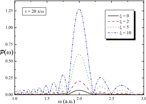
Figure 3: Transition probability for the spiked harmonic oscillator, as functions of the field frequencyω and different parametersξintroduced in (79). We consider the transition from the energy leveln= 2 tom= 3 to first-order perturba-tion theory with respect to the external laser field.The field amplitude is taken to be weakE0= 0.005 a.u. and the
cou-pling constant is chosen asλ= 0.5. The pulse lengthτ and the frequencyωare indicated in the figure.
we would havehφn|ηxη−1 φmi. Now for (80) we would
have that hφn|ηxη−1φmi=hφn|x φmiforn6=m, such
that no effect would be visible in the transition amplitude to first order.
Let us therefore take instead the transformation ˜η = exp(−ξp2). We then compute the canonical variables to
˜
X=x−i2ξp and P˜ =p. (81)
For the corresponding non-Hermitian systemH(x, p) =
hSHO( ˜X,P˜) we evaluate next the transition amplitude
for φ0.2
2 →φ03.2 withλ= 0.5, subjected to a
monochro-matic linearly polarized electric field E(t) = E0sin(ωt) and depict the result in figure 3.
As expected we obtain the main contribution for the transition atε0.2
3 −ε02.2= 2. The valueξ= 0 is perfectly
reasonable and corresponds to addingXE(t) toH, with
X given in (80) for the reasons outlined above. However, for large enough values ofξwe observe that the transition probability becomes larger than 1, which is of course in-consistent and unphysical. Therefore to addxE(t) toH
is meaningless in our framework, unless xcan be chosen to be an observable in the non-Hermitian system.
C. The -x4
potential
A further interesting Hamiltonian arises when we spec-ify in equation (1) the parameterN = 4, which involves a potential which is unbounded from below. Recently Jones and Mateo [8] established that this Hamiltonian is in fact isospectral to the Hermitian Hamiltonian
˜
H=p2+ 4g2x4−2gx for x, g∈R (82)
This Hamiltonian is of great interest as it serves as a sim-plified version for the −φ4 quantum field theory, which
may for instance be used to mimic the Higgs mechanism. To obtain the Hamiltonian (82) from (1) withN = 4 one needs to pass via two auxiliary Hamiltonians as follows
H(z)−→z(x)H(x)−→η h=h† −→F T H˜. (83)
All manipulation in (83) are spectrum preserving. In the first step the general idea [6] was used to map the con-tour from within the wedgesWLandWRback to the real
axis. As discussed in section II A 1 there are many pos-sible parameterization, which guarantee the appropriate boundary condition. Unfortunately, there is no construc-tive method to select out the most useful contour within the wedges and this choice remains a matter of inspired guess work [8]. Here the best choice is guided by the de-sire to be able to construct a similarity transformationη, which maps the non-Hermitian HamiltonianH adjointly into a Hermitian Hamiltonian h. Hitherto, this proce-dure was only successful in an exact manner for the class of Hamiltonians in (1) withN = 4, in which case η can be constructed exactly either by operator methods [8], differential-equation techniques [45] or Moyal products
[39]. Even for the next exampleN = 6 the same trans-formation used as in [8] does not yield an exact similar-ity transformation [51]. The last step in (83) in the case
N= 4 is to transformhinto the Hamiltonian ˜H(82) via a Fourier transformation.
Concretely, we exchange now the constantgbyεin (1) withN = 4 and obtainH =−d2/dz2−εz4 thereafter.
Using now the parameterizationz1(x) as defined in (7) one obtains the non-Hermitian Hamiltonian
Hx4= ˆp2−2pˆ+αxˆ2−α +ig
{x,ˆ pˆ2}
2 −2αxˆ
, (84)
The domain ofHx4
is now the entire real axis, whereα= 16εand the coupling constantg has been introduced to separate off the non-Hermitian part [8, 39]. Next we want to computeη by means of Moyal products. For this we have to convertH first into a real valued function and have to substitute the anti-commutator with the Moyal products. Thus we have to replace{x,ˆ pˆ2} by x ⋆ p2+ p2⋆ x = 2xp2. Subsequently we can use (64) and the
differential equation (67) for the Hamiltonian (84) in the unknown quantityη2(x, p) becomes
0 = 4gp2xη2−8gxαη2−4xα∂pη2 (85)
−∂xη2+ 4p∂xη2+ 2gp∂p∂xη2−gx∂x2η2.
We can solve this by
η2=eg p
3
3α−2g p, (86)
such thatη=eg p
3
6α−g p. From (24) we obtain thereafter
the Hermitian Hamiltonian
hx4 = ˆp2−pˆ
2 +α xˆ
2
−1
+g2 pˆ
2−2α2
4α . (87)
Let us compare how these expressions are obtained by means of operator identities. In principle we have to make a general ansatz to findq, but having already found
η we can simply extract it from (86)
q= g 3αp
3
−2gp (88)
and verify the corresponding expressions. From (84) we find that
hx04 = ˆp2−
ˆ
p
2 +α xˆ
2
−1
. (89)
Next we compute then-fold commutators
c(1)q (hx
4
0 ) = 4igαx−ig{x, p2} (90) c(2)q (hx
4
0 ) =−g2
2
α p
2
−2α2
(91)
c(3)q (hx
4
0 ) = 0. (92)
the generic expression (60) for the non-Hermitian Hamil-tonian gives (84).
Now the non-Hermitian system in terms of its canoni-cal variables
X =x+ ig 2a p
2
−2a
and P =p, (93)
results fromHx4
(x, p) =hx4
(X, P). In addition we verify
hx4
(x, p) = (Hx4
)†(X, P).
In this case it suffices to chooseP =pas an observable to make the metric unique. Note also that it is not possi-ble to demandX =xto be an observable as we can not find a functionf(x) such that all functional dependence onpis eliminated from the termq+f(hx4
0 ).
V. CONCLUSIONS
Given a non-Hermitian time-independent Hamiltonian
H, we argued that the analogue of the Stark-LoSurdo Hamiltonian should be
Hl(t) =H+XE(t), (94)
where X = η−1xη is the position operator in the
non-Hermitian system. As we have shown when we simply addxE(t) toH, we obtain unphysical results unlessxis an observable in the non-Hermitian system. However, we also demonstrated that this is not always possible andx
is often degraded to be a mere auxiliary variable in the non-Hermitian system.
As in the time-independent scenario we saw that once the similarity transformation is known, one can easily translate all the relevant calculations into the Hermitian system. The situation is less straightforward when the transformation η and therefore the Hermitian system is not known. In that case one may take our expressions as benchmarks and think of various different approximation schemes, such as standard perturbation theory, a pertur-bation via theC-operator, Floquet type approximations for periodic potentials etc.
From what has been said one may adopt a rather pes-simistic standpoint and conclude that in the end the non-Hermitian formulation is in most cases a mere change of metric of a well posed Hermitian problem. Nonetheless, even leaving the technical difficulty aside to establish the precise relation between these conceptually different for-mulations, it has been successfully argued that the
non-Hermitian formulation is often more natural and simpli-fies computations [52, 53]. For an atomic physicist this is of course a natural scenario when we compare these al-ternative formulations with treatments in various gauges, which are also just different ways to express the same physical quantity. It is a well established fact that differ-ent choices of gauges often drastically simplify problems in that context and allow for a more intuitive interpreta-tion. For instance, tunneling processes can be visualized and interpreted more easily in the length gauge formu-lation, since then one may picture the problem in terms of a time-dependent effective potential barrier, whereas all other gauges would obscure this intuitive physical in-terpretation. Furthermore, phenomena occurring in the context of high frequency fields are most intuitively un-derstood when viewed in a time-dependent dichotomous potential in the Kramers-Henneberger gauge
Let us conclude by commenting on some of the immedi-ate open problems, which follow from what we discussed. Concerning the time-dependent treatment it would be in-teresting to change the current set-up by allowing η to be time-dependent.
Having entirely focussed on the pseudo-Hermitian na-ture of the Hamiltonians involved, we want to conclude with a final comment on the role played byPT-symmetry in the time-dependent setting. When [PT, η] = 0 the termXE(t) is onlyPT-symmetric whenE(−t) =−E(t). This means thatPT-symmetry depends on the explicit form of the laser pulse. Taking for instance a typical pulse for a laser field with frequency ω, amplitude E0
and Gaussian enveloping function f(t), that is of the form E(t) = E0sin(ωt)f(t), the term xE(t) would be
PT-invariant. However, the perfectly legitimate replace-ment sin(ωt) → cos(ωt) in this field would break the
PT-invariance. Recall that in this context the electric field is treated classically. For a discussion of PT -symmetry for a full quantum electrodynamic setting we may refer to [54, 55]. However, for the physical appli-cations we dealt with in this manuscript,PT-invariance is not a relevant issue, since the pulse is always chosen such that HΦ(0) = εΦ(0) and HΦ(τ) = εΦ(τ). The consequences of PT-symmetry on the eigenvalue prob-lem is therefore only important when considering the full time-independent eigenvalue problem (32). To investi-gate this full solution of (32), the consequences on the non-Hermitian counterpart with its dressed states [32] would be extremely interesting [56].
[1] H. Friedrich and D. Wintgen, Interfering resonances and bound states in the continuum, Phys. Rev.A32, 3231– 3243 (1985).
[2] H. Geyer, D. Heiss, and M. Znojil (guest editors), Special issue dedicated to the physics of non-Hermitian operators (PHHQP IV) (University of Stellenbosch, South Africa,
23-25 November 2005), J. Phys.A39, 9965–10261 (2006). [3] C. Figueira de Morisson Faria and A. Fring, Time evo-lution of non-Hermitian Hamiltonian systems, J. Phys.
A39, 9269–9289 (2006).
Rev. Lett.80, 5243–5246 (1998).
[5] C. M. Bender and S. A. Orszag, Advanced Mathematical Methods for Scientists and Engineers, MacGraw-Hill, New York (1978).
[6] A. Mostafazadeh, Pseudo-Hermitian Description of PT-Symmetric Systems Defined on a Complex Contour, J. Phys.A38, 3213–3234 (2005).
[7] H. F. Jones and J. Mateo, Pseudo-Hermitian hamiltoni-ans: a tale of two potentials, Czech. J. Phys.55, 1117– 1122 (2005).
[8] H. F. Jones and J. Mateo, An Equivalent Hermitian Hamiltonian for the non-Hermitian−x4
Potential, Phys. Rev.D73, 085002(4) (2006).
[9] J. A. C. Weideman, Spectral differentiation matrices for the numerical solution of Schr¨odinger’s equation, J. Phys.
A39, 10229–10237 (2006).
[10] C. M. Bender, D. C. Brody, and H. F. Jones, Complex Extension of Quantum Mechanics, Phys. Rev. Lett.89, 270401(4) (2002).
[11] P. Dorey, C. Dunning, and R. Tateo, Spectral equiva-lences from Bethe ansatz equations, J. Phys.A34, 5679– 5704 (2001).
[12] K. C. Shin, Eigenvalues of PT-symmetric oscillators with polynomial potentials, J. Phys.A38, 6147–6166 (2005). [13] E. Wigner, Normal form of antiunitary operators, J.
Math. Phys.1, 409–413 (1960).
[14] S. Weigert, PT-symmetry and its spontaneous break-down explained by anti-linearity, J. Opt. B: Quantum Semiclass. Opt.5, S416–S419 (2003).
[15] S. Weigert, Detecting brokenPT-symmetry, J. Phys.
A39, 10239–10246 (2006).
[16] Z. Ahmed, Pseudo-Hermiticity of Hamiltonians under imaginary shift of the coordinate: real spectrum of com-plex potentials, Phys. Lett.A290, 19–22 (2001). [17] A. Mostafazadeh, Pseudo-Hermiticity versus
PT-Symmetry II: A complete characterization of non-Hermitian Hamiltonians with a real spectrum, J. Math. Phys.43, 2814–2816 (2002).
[18] F. G. Scholtz, H. B. Geyer, and F. Hahne, Quasi-Hermitian Operators in Quantum Mechanics and the Variational Principle, Ann. Phys.213, 74–101 (1992). [19] W. Heisenberg, Quantum theory of fields and elementary
particles, Rev. Mod. Phys.29, 269–278 (1957).
[20] A. Mostafazadeh, Pseudo-Hermiticity versus PT symme-try. The necessary condition for the reality of the spec-trum, J. Math. Phys.43, 205–214 (2002).
[21] A. Mostafazadeh, Pseudo-Hermiticity versus PT-Symmetry III: Equivalence of pseudo-Hermiticity and the presence of anti-linear symmetries, J. Math. Phys.43, 3944–3951 (2002).
[22] A. Mostafazadeh, Exact PT-Symmetry Is Equivalent to Hermiticity, J. Phys.A36, 7081–7092 (2003).
[23] A. Mostafazadeh, Pseudo-Hermiticity and Generalized PT- and CPT-Symmetries, J. Math. Phys.44, 974–989 (2003).
[24] S. Weigert, Completeness and orthonormality in PT -symmetric quantum systems, Phys. Rev.A68, 062111(4) (2003).
[25] I. Rotter and A. F. Sadreev, Avoided level crossing, di-abolic points in the complex plane in a double quantum dot, Phys. Rev.E71, 0362271(14) (2005).
[26] E. Persson, T. Gorin, and I. Rotter, Decay rates of res-onance states at high level density, Phys. Rev. E54, 3339–3351 (1996).
[27] M. Leone, A. Paoletti, and N. Robotti, A simultaneous discovery: The case of Johannes Stark and Antonio Lo Surdo, Phys. Perspect.6, 271–294 (2004).
[28] H. Silverstone, High-order perturbation theory and its application to atoms in strong fields, Atoms in Strong Fields, ed. C.N. Nicolaides (Plenum Press, New York) , 295–311 (1990).
[29] A. Fring, V. Kostrykin, and R. Schrader, On the absence of bound-state stabilization through short ultra-intense fields, J. Phys.B29, 5651–5671 (1996).
[30] C. Figueira de Morisson Faria, A. Fring, and R. Schrader, Analytical treatment of stabilization, Laser Physics 9, 379–387 (1999).
[31] C. Figueira de Morisson Faria, A. Fring, and R. Schrader, Existence criteria for stabilization from the scaling be-haviour of ionization probabilities, J. Phys.B33, 1675– 1685 (2000).
[32] M. Born and V. Fock, Beweis des Adiabatensatzes, Zeit. f¨ur Physik51, 165–180 (1928).
[33] A. Fleischer and N. Moiseyev, Adiabatic theorem for non-hermitian time-dependent open systems, Phys. Rev.
A72, 032103(11) (2005).
[34] M. Lewenstein, P. Salieres, A. L’Huillier, and P. Antoine, Study of the Spatial and Temporal Coherence of High Or-der Harmonics, Adv. At. Mol. Opt. Phys.41, 83 (1999). [35] W. Becker, F. Grasbon, R. Kopold, D. Milosevic, G. Paulus, and H. Walther, Above-threshold ionization: from classical features to quantum effects, Adv. At. Mol. Opt. Phys.48, 35–98 (2002).
[36] C. Joachain, M. D¨orr, and N. Kylstra, High Intensity Laser-Atom Physics, Adv. At. Mol. Opt. Phys.42, 225– 286 (2000).
[37] C. M. Bender, D. C. Brody, and H. F. Jones, Extension of PT-symmetric quantum mechanics to quantum field the-ory with cubic interaction, Phys. Rev.D70, 025001(19) (2004).
[38] A. Mostafazadeh, PT-Symmetric Cubic Anharmonic Os-cillator as a Physical Model, J. Phys.A38, 6557–6570 (2005).
[39] C. Figueira de Morisson Faria and A. Fring, Isospectral Hamiltonians from Moyal products, Czech. J. Phys.56, 899-908 (2006).
[40] E. Caliceti, F. Cannata, and S. Graffi, Perturbation theory of PT-symmetric Hamiltonians, J. Phys.A39, 10019–10027 (2006).
[41] F. G. Scholtz and H. B. Geyer, Operator equations and Moyal products – metrics in quasi-hermitian quantum mechanics, Phys. Lett.B634, 84–92 (2006).
[42] F. G. Scholtz and H. B. Geyer, Moyal products – a new perspective on quasi-hermitian quantum mechanics, J.Phys.A39, 10189–10205 (2006).
[43] D. B. Fairlie, Moyal brackets, star products and the gen-eralised Wigner function, J. of Chaos, Solitons and Frac-tals10, 365–371 (1999).
[44] A. Mostafazadeh, Differential Realization of Pseudo-Hermiticity: A quantum mechanical analog of Einstein’s field equation, J. Math. Phys.47, 072103(11) (2006). [45] C. M. Bender, D. C. Brody, J.-H. Chen, H. F. Jones,
K. A. Milton, and J. C. Ogilvie, Equivalence of a com-plex PT-symmetric quartic Hamiltonian and a Hermitian quartic Hamiltonian with an anomaly, Phys. Rev.D74, 025016(10) (2006).
(2004).
[47] H. Jones, On pseudo-Hermitian Hamiltonians and their Hermitian counterparts, J. Phys. A38, 1741–1746 (2005).
[48] E. Witten, Constraints on supersymmetry breaking, Nucl. Phys.B202, 253–316 (1982).
[49] F. Cooper, A. Khare, and U. Sukhatme, Supersymme-try and quantum mechanics, Phys. Rep. 251, 267–385 (1995).
[50] M. Znojil, PT-symmetric harmonic oscillators, Phys. Lett.A259, 220–223 (1999).
[51] C. Figueira de Morisson Faria, A. Fring, and H. Jones, unpublished notes.
[52] C. M. Bender, J.-H. Chen, and K. A. Milton, PT-symmetric versus Hermitian formulations of quantum mechanics, J. Phys.A39, 1657–1668 (2006).
[53] C. M. Bender, D. C. Brody, H. F. Jones, and B. K. Meis-ter, Faster than Hermitian Quantum Mechanics, quanth-ph/0609032 (2006).
[54] K. A. Milton, Anomalies in PT-symmetric quantum field theory, Czech. J. Phys.54, 85–91 (2004).
[55] C. M. Bender, I. Cavero-Pelaez, K. A. Milton, and K. V. Shajesh, PT-symmetric quantum electrodynam-ics, Phys. Lett.B613, 97–104 (2005).