A Variational Approach to the Evolution of Radial Basis Functions for Image Segmentation

City, University of London Institutional Repository

Citation:

Slabaugh, G. G., Dinh, Q. and Unal, G. B. (2007). A Variational Approach to the

Evolution of Radial Basis Functions for Image Segmentation. In: IEEE Conference on

Computer Vision and Pattern Recognition, 2007 (CVPR '07). (pp. 1-8). IEEE. ISBN

1424411793

This is the accepted version of the paper.

This version of the publication may differ from the final published

version.

Permanent repository link:

http://openaccess.city.ac.uk/6134/

Link to published version:

http://dx.doi.org/10.1109/CVPR.2007.383013

Copyright and reuse: City Research Online aims to make research

outputs of City, University of London available to a wider audience.

Copyright and Moral Rights remain with the author(s) and/or copyright

holders. URLs from City Research Online may be freely distributed and

linked to.

City Research Online:

http://openaccess.city.ac.uk/

[email protected]

A Variational Approach to the Evolution of Radial Basis Functions for Image

Segmentation

Greg Slabaugh

, Quynh Dinh

, Gozde Unal

1

_{Intelligent Vision and Reasoning Department}

_{Computer Science Department}

Siemens Corporate Research

Stevens Institute of Technology

Princeton, NJ USA

Hoboken, NJ USA

{greg.slabaugh, gozde.unal}@siemens.com [email protected]

Abstract

In this paper we derive differential equations for evolv-ing radial basis functions (RBFs) to solve segmentation problems. The differential equations result from applying variational calculus to energy functionals designed for im-age segmentation. Our methodology supports evolution of all parameters of each RBF, including its position, weight, orientation, and anisotropy, if present. Our framework is general and can be applied to numerous RBF interpolants. The resulting approach retains some of the ideal features of implicit active contours, like topological adaptivity, while requiring low storage overhead due to the sparsity of our representation, which is an unstructured list of RBFs. We present the theory behind our technique and demonstrate its usefulness for image segmentation.

1. Introduction

Active contours have enjoyed copious success in com-puter vision since their introduction [7], and have since been the subject of intensive research activity. These meth-ods have found application in numerous important problems such as image segmentation, 3D scene reconstruction, and object tracking. Part of their success is that they provide a structured approach (via energy minimization) to deform a contour or surface – a problem that comes up frequently in computer vision.

In the context of image segmentation, active contours de-form based on various image-based and internal forces so that the contour’s edges match object or region boundaries in the image, while maintaining smoothness. The smooth-ness, or regularization terms, provide robustness to noise while providing a measured approach to handling missing or low-confidence data. A typical application of an active contour will start with an initial contour, which is then

itera-tively deformed until it converges to a solution that balances the forces acting on the contour. Typically, these forces re-sult from analytic expressions that are derived using varia-tional calculus applied to an energy minimization problem; however, it is possible to define the forces directly without using an energy formulation.

In the active contour literature, earlier methods repre-sented the contour using a topologically fixed paramet-ric representation, such as a polyline, spline, etc., spec-ified by a fixed number of control points. Such repre-sentations are simple and efficient to implement, however, they lack straightforward mechanisms for topological con-trol. Often in segmentation problems, the topology of the problem is unknown a priori, and the contour must break apart or merge during evolution. While various au-thors have since presented methods that provide topological changes [8, 10, 5], the implementation is somewhat compli-cated and not natural to the parametric representation.

Recently there has been much interest in implicit ac-tive contours, or level set methods, which represent the sur-face as a level set of a higher dimensional embedding func-tion [1, 2, 14, 16]. The primary advantage of this repre-sentation is that topological changes occur naturally in this framework; by manipulating the embedding function, the level set that represents the contour can innately split or merge without requiring any specialized implementation to handle topological changes. However, the embedding func-tion must be updated on a dense set of points, requiring significant storage, even when using efficient narrowband techniques [9].

embedding function can be computed. These approaches then, provide a methodology to move the points (and corre-spondingly, update the embedding function) to deform the active contour to solve the segmentation problem. Such ap-proaches have been demonstrated to provide the topological flexibility of level set methods with the low storage require-ments of parametric representations, and offer much flexi-bility in terms of RBF placement and interaction.

This paper is related to such work; however, there are notable differences. These previous methods start with the force definition rather than deriving the forces through an energy formulation. We present this derivation, which pro-vides a stronger theoretical framework for the technique. In addition, from this derivation we observe how it is possi-ble to evolveallattributes of each RBF, whereas previous work only evolved the RBF positions. For example, in the case of an anisotropic Gaussian RBF interpolant, we show how to evolve the position, weight, orientation, and stan-dard deviations of each RBF, resulting in a set of coupled differential equations that drive the active contour. In ad-dition, we derive equations for region-based segmentation problems in addition to the edge-based segmentation prob-lems addressed previously. Our methodology is general, al-lowing other RBF interpolants and curve evolutions to be utilized in our framework.

The rest of this paper is organized as follows. In Sec-tion 2 we present the mathematical details of our frame-work, deriving the RBF update equations from an energy functional. Next, in Section 3 we complete the derivation by considering anisotropic radial basis functions. Then, in Section 4 we provide some implementation details, includ-ing how we add and merge RBFs durinclud-ing evolution. In Sec-tion 5 we show some initial results that demonstrate the use-fulness of our method, and offer some concluding remarks in Section 6.

2. Variational RBF Evolution

In this section we derive our RBF evolution equations, resulting in a set of coupled differential equations that drive the evolution. We begin by considering region-based image segmentation.

2.1. Region-based image segmentation

In region-based segmentation methods, the evolution of the active contour is based on the attributes of entire regions in the image. These attributes can include intensity, color, texture, probabilities, etc., but in this paper we focus on intensity. These methods model the image as being com-posed of distinct regions, each with its own statistics, which are used to deform the active contour towards the region boundaries. This is notably different than boundary-based segmentation methods, where the evolution depends on

lo-cal image gradients. In this sense, region-based segmenta-tion methods are more global and more robust to noise than edge-based methods.

Perhaps the most well-known region-based model is the Mumford-Shah functional [13], which models the image re-gions as piece-wise smooth functions. For example, in the case of two regionsRinside the contourCand the region

RC_{outside the contour,}

E(f, C) = Z

R

(I(x)−fR(x))2dx (1) +

Z

RC

(I(x)−fRC(x))2dx+

Z

Ω\C

|∇f|2_dx+γ

Z

C ds,

whereE(f, C)is the energy of the contour,I(x)is the im-age intensity at pixelx, andf is a piecewise smooth func-tion, consisting of regionsfR(x)insideCandfRC(x)

out-sideC, and the last term is a regularization term weighted by a constantγ. While there are good active contour meth-ods to solve the Mumford-Shah functional [17], the piece-wise constant model of Chan-Vese [2] is a powerful approx-imation that replaces the piecewise smooth functionf with piecewise constant functions in each region. This simplified form can be expressed as

E(C) = Z

R

(I(x)−µin)2dx+ Z

RC

(I(x)−µout)2dx+γ Z

C ds,

(2) whereµinis the average intensity inside theCandµout is

the average intensity outsideC. Many other variations of the Chan-Vese functional exist, for example, using various statistics other than or in addition to the mean.

In both the level set formulation and ours based on RBFs, the contourC∈Ωis represented by the zero level set of a Lipschitz functionφ: Ω→ <, such that

C = {x∈Ω :φ(x) = 0}, R = {x∈Ω :φ(x)<0}, RC = {x∈Ω :φ(x)>0}

Now in our case, we model the embedding functionφ(x)

usingN radial basis functionsψ(x, gi1· · ·giM)[18] as

φ(x) =P(x) + N X

i=1

wiψi(x, gi1· · ·giM), (3)

whereψi(x, gi1· · ·giM)is theith RBF parameterized by M variablesgi1· · ·giM,wi is the weight on theith RBF,

andP(x)is a polynomial term that spans the null space of the basis function.

Using the Heaviside function,

H(z) =

1, z≥0

and the Dirac delta functionδ(z) = _dzdH(z), the energy of Equation 2 can be reexpressed as

E(φ(w,g)) = Z

Ω

(I(x)−µin)2H(φ(x))dx (5) +

Z

Ω

(I(x)−µout)2(1−H(φ(x)))dx+γ Z

Ω

δ(φ(x))|∇φ(x)|dx,

where w = [w1. . . wN]T, and g = [gij], where i = 1· · ·N,j= 1· · ·M.

Under this formulation of the problem, we would like to derive the variation of the energy with respect to the RBF parametergij, as well as the RBF weight,wi. Using the

chain rule, we derive

∂E ∂gij

= Z

Ω

(I(x)−µin)2δ(φ(x)) ∂φ ∂gij dx − Z Ω

(I(x)−µout)2δ(φ(x)) ∂φ ∂gij dx +γ Z Ω div ∇φ

|∇φ|

δ(φ(x)) ∂φ

∂gij

dx, (6)

which simplifies to the contour integral,

∂gij ∂t = ∂E ∂gij = Z C

(I(x)−µin)2−(I(x)−µout)2 +γdiv

_∇φ

|∇φ|

_∂φ ∂gij dC, (7) and similarly, ∂wi ∂t = ∂E ∂wi = Z C

(I(x)−µin)2−(I(x)−µout)2 +γdiv

∇φ

|∇φ|

_∂φ

∂wi

dC. (8)

We note that these expressions take the form

R C

∂E ∂φ

∂φ

∂pdC, where p is gij or wi. This form results

from the functional composition that resulted in application of the chain rule. Conceptually, these equations state that to determine the update of a parameter of an RBF, we must traverse the contour C, accumulating gradients at each point. That is, each point on the zero level set contributes to the update of the RBF parameters, which is intuitive, given that in general, the RBF influences every point on the zero level set. Unlike standard level set update equations, the integral in Equations 7 and 8 combines measurements from all points along the contour [15], providing increased robustness to noise. We note that our formulation of the problem is notably different than [11], where the RBFs are fixed to the zero level set and the evolution of an RBF does not consider the influence of the RBF on all other points on the zero level set. Likewise, this approach differs from [12] as it is based solely on gradient descent and does not require

solving linear systems of equations for the RBF locations. Unlike [11, 12, 6], our method provides a generalized simple way to updateallparameters of the basis function, including the weights, position, orientation, anisotropy, etc. This of course depends on the functional form of φ, for which we consider for various basis functions in Section 3. We note that each iteration of all RBFs is orderO(LM N), whereLis the number of pixels on the zero level set, and

M andN are given above.

2.2. Boundary-based image segmentation

From the previous section, we observed that the energy minimization resulted in the formR

C ∂E ∂φ

∂φ

∂pdC. In general,

one can utilize this relationship to transform any level set flow or curve evolution into an RBF evolution in our frame-work. For boundary-based image segmentation, we deduce a similar expression for the geodesic flow [1],

∂gij ∂t = ∂E ∂gij = Z C

[F κ|∇φ| − ∇F· ∇φ] ∂φ

∂gij dC ∂wi ∂t = ∂E ∂wi = Z C

[F κ|∇φ| − ∇F· ∇φ] ∂φ

∂wi dC,

whereF(I(x))is a function of an edge detector response, such asF = _1+|∇1_I|2 andκis the curvature of the active

contour at pointx. We note often with boundary-based seg-mentations, it is helpful to run a GVF diffusion [20] on the vector field∇Fbefore evolving the active contour.

3. Radial Basis Functions

In the previous section, we derived the basic equations for evolution of radial basis functions to achieve either a region-based or boundary-based image segmentation. How-ever, the complete derivation depends on the RBFs cho-sen and their derivatives. In this section, we consider the use of anisotropic Gaussian RBFs. We note however, that our framework is quite general, and that any RBF with an analytic derivative can be used. We choose to work with anisotropic basis functions for two reasons: first, they can better approximate sharp corners [4], and second, they are a more general form of the isotropic basis function. Also note that in the presentation below we consider 2D RBFs, however, the method straightforwardly generalizes to 3D.

3.1. Anisotropic Gaussian RBFs

The equation for a 2D anisotropic Gaussian centered at point (cx, cy), standard deviationσx, σy, and orientation

angleθhas the functional form

ψ(x, y) = 1 2πσxσy

exp ₋₁

2σ2

xσy2

a1(x−cx)2

where

a1 = σ2xcos

2_θ+σ2

ysin

2_θ

(9)

a2 = (σy2−σ

2

x) cosθsinθ (10) a3 = σ2xsin

2_θ+σ2

ycos

2_{θ (11)}

This RBF is described by theM = 5five parameters,

gj = [cx, cy, σx, σy, θ]T. To implement our RBF flows, we

must take the derivative of the RBF with respect to these parameters. Doing so yields the equations,

∂ψ ∂cx

= ψ·

_a

1X−a2Y

σ2

xσ2y

(12)

∂ψ ∂cy

= ψ·

_−a

2X+a3Y

σ2

xσy2

(13)

∂ψ

∂θ = ψ· − X2∂a1

∂θ −2XY ∂a2

∂θ +Y

2∂a3

∂θ 2σ2

xσ2y

!

(14)

∂ψ ∂σx

= −ψ

σx +ψ·

_a

1X2−2a2XY +a3Y2

σ3

xσ2y

− 1

2σ2

xσy2

X2∂a1 ∂σx

−2XY ∂a2 ∂σx

+Y2∂a3 ∂σx

(15)

∂ψ ∂σy

= −ψ

σy +ψ·

_a

1X2−2a2XY +a3Y2

σ2

xσy3

− 1

2σ2

xσy2

X2∂a1 ∂σy

−2XY∂a2 ∂σy

+Y2∂a3 ∂σy

, (16)

where

X = (x−cx) (17)

Y = (x−cy) (18)

∂a1

∂θ = −2(σ

2

x−σ

2

y) cosθsinθ (19) ∂a2

∂θ = −(σ

2

x−σ

2

y)(cos

2_θ−sin2_{θ) (20)}

∂a3

∂θ = 2(σ

2

x−σ

2

y) cosθsinθ (21) ∂a1

∂σx

= 2σxcos2θ (22)

∂a2

∂σx

= −2σxcosθsinθ (23) ∂a3

∂σx

= 2σxsin2θ (24)

∂a1

∂σy

= 2σysin2θ (25)

∂a2

∂σy

= 2σycosθsinθ (26)

∂a3

∂σy

= 2σycos2θ (27)

(28)

Putting it all together gives the following set of cou-pled ordinary differential equations (ODEs) that drive the

ith RBF:

dcix dt =

Z

C

Dwiψi·

ai1Xi−ai2Yi σ2 ixσ 2 iy ! dC (29) dciy dt = Z C

Dwiψi·

−ai2Xi+ai3Yi σ2 ixσ 2 iy ! dC (30) dwi dt = Z C

DψidC (31)

dθi dt =

Z

C Dwi·

ψi· − X2

i ∂ai1

∂θi −2XiYi

∂ai2

∂θi +Y 2

i ∂ai3

∂θi

2σ2

ixσiy2

! dC (32) dσix dt = Z C Dwi· (

−ψi

σix +ψi·

"

ai1Xi−2ai2XiYi+ai3Yi2 σ3

ixσ2iy

− 1

2σ2

ixσ2iy

Xi2 ∂ai1

∂σix

−2XiYi ∂ai2

∂σix +Yi2

∂ai3

∂σix #) dC(33) dσiy dt = Z C Dwi· (

−ψi

σiy +ψi·

"

ai1Xi2−2ai2XiYi+ai3Yi2 σ2

ixσ3iy

− 1

2σ2

ixσ2iy

X_i2∂ai1 ∂σiy

−2XiYi ∂ai2

∂σiy

+Y_i2∂ai3 ∂σiy

#)

dC (34)

where

Xi = (x−cix) (35) Yi = (y−ciy) (36)

and for region-based segmentation,

D=

(I(x)−µin)2−(I(x)−µout)2+γdiv _∇φ

|∇φ|

(37) while for boundary-based segmentation,

D= [F κ|∇φ| − ∇F· ∇φ] (38) While these systems of equations may look complex, they contain many repeated terms and are easily imple-mented on a computer.

(a) (b) (c) (d)

(e) (f) (g) (h)

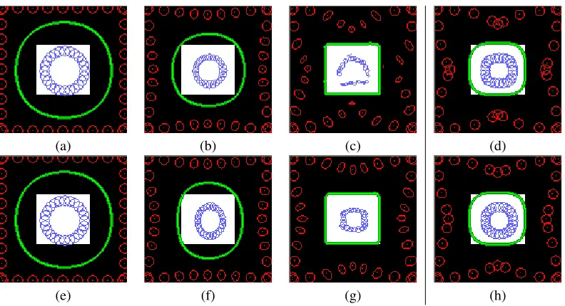
Figure 1. RBF evolution for segmentation of a white square on a black background. Top row: Chan-Vese region-based flow. Bottom row: geodesic boundary-based flow. The evolution is shown starting at initialization ((a) and (e)), at an intermediate stage ((b) and (f)), and at convergence ((c) and (g)) for the evolution of all RBF parameters, including anisotropy. For comparison, in (d) and (h) we show the isotropic RBF evolution result of evolving just the weights and RBF centers. The isotropic RBFs are unable to capture the sharp corners of the object.

figure, we show the initialization, which consists of a con-tour, shown in green, which is the zero level set of the im-plicit functionφ(x, y). The implicit function is represented as a summation of RBFs. Negative weighted RBFs are ren-dered in blue, while positive weighted RBFs are renren-dered in red. The ellipse around each RBF is a visualization of the anisotropy. Initially, the RBFs are all isotropic and are rendered as circles. In (b), we show the result at an inter-mediate stage of the segmentation after 10 iterations of the ODEs and in (c), we show the final result after convergence after 25 iterations. Note the RBFs changed their positions, weights, and anisotropy to produce the result in (c), which provides an excellent segmentation of the data. For compar-ison, in (d) we show the evolution of just the RBF weights and center positions. In this case, the isotropic RBFs are un-able to capture the sharp corners of the object. The bottom row of the figure reruns this experiment using the geodesic boundary based flow, which provides similar results.

3.2. Other Basis Functions

We note any RBF interpolant that has an analytic deriva-tive can be used in our framework, including multi-order [3] and Wendland’s [19] RBFs. Experimentally, we have ob-served best results using RBFs that decay from their cen-ter location. However, due to page constraints we do not present derivations or results for these other RBFs.

4. Implementation

In this section, we provide some implementation details regarding our RBF evolution approach to image segmenta-tion.

4.1. Overall approach

Our approach requires an initialization, which consists of a set of RBFs that define an initial contour for segmentation. The positions of these RBFs can be placed manually by the user, or automatically by placing positive-weighted RBFs on the image border or in a large ring around the image cen-ter, and negative-weighted RBFs in the center of the image, resulting in an initial contour on the image. The initializa-tion is flexible, as the initial contour can be inside, outside, or both inside and outside the object being segmented, as we will show in the examples of Section 5. Given this ini-tial contour, we then evolve the RBFs using Equations 29 to 34. These ODEs update the RBF parameters, and conse-quently update the curve as well to solve the segmentation problem. One can check for convergence of the ODEs by monitoring the energy ofE.

4.2. Merging and adding RBFs

(a) (b) (c)

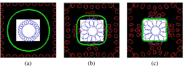
Figure 2. Adding and removing RBFs.

(a) (b) (c)

Figure 3. An example demonstrating a topological change of the contour.

the jth RBF by [cjx, cjy, σjx, σjy, θj] and weight wj, i 6= j. If the distance between two RBFs, dij = p

(cix−cjx)2+ (ciy−cjy)2becomes less than a

thresh-old TM (typically 7 pixels in our experiments), then the

RBFs are combined by deleting them and replacing them with a new RBF,[1₂(cix+cjx),1₂(ciy+cjy), σix+σjx, σiy+ σjy, θi+θj]and weightwi+wj. This new RBF is a sum of

the two RBFs being merged and centered halfway between. We add RBFs at locations where the gradient of the im-plicit function is high. However, we do not want to add an RBF too close to an already existing RBF. To satisfy these constraints, we form a functionA(x, y) = _max(∇φ_∇(_φx,y_(x,y) ₎₎ ·

S(x, y), where _max(∇φ_∇(_φx,y_(x,y) ₎₎ is the normalized gradient of the implicit function andS(x, y)is a splat buffer formed as

S(x, y) =Y i

1−e−[(cix−x)2+(ciy−y)2]/(2σ2) ₍₃₉₎

whereσis a standard deviation of a 2D Gaussian function (set to 15 for our experiments). The splat buffer is close to one where there are no RBFs, and decreases to zero near RBF centers. Therefore, the functionA(x, y)is large where there are no RBFs and the gradient of the implicit function is high. We scanA(x, y), and add an RBF at the position

(x, y)whereA(x, y)has a value above a threshold,TA

(typ-ically 0.65 in our experiments). This gives us a new RBF that is not too close to an existing RBF, yet is located at a point of high gradient in the implicit function. The thresh-oldTAprevents us from adding too many constraints where

they are not really needed. The weight of this newly added

isotropic RBF is initially zero; subsequent iterations of the ODEs will update its weight and anisotropy.

An example showing the adding and merging of RBFs is provided in Figure 2. Here, the method automatically places the RBFs where they will help the most in modeling the curve geometry, and ODEs update the RBFs to solve the segmentation problem. Using these mechanisms, topo-logical changes of the contour also come naturally in our framework. An example of this is provided in Figure 3.

5. Results

In this section we present some results demonstrating the effectiveness of our proposed method in segmentation of various images.

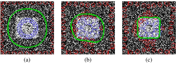
In Figure 4, we repeat the experiment of Figure 2, this time on a very noisy image corrupted by Gaussian white noise. Here the image was formed by setting the back-ground pixels to 0, the foreback-ground pixels to 200, and adding in Gaussian white noise of unit standard deviation, where the noise was then multiplied by 200. The resulting image was clipped to [0, 255], and has a very noisy appearance. The evolution of our anisotropic RBFs are shown from the initialization (a), at an intermediate stage (b), and upon con-vergence (c). The region-based active contour does an ex-cellent job of segmenting the object despite the low signal to noise ratio. In each of these examples, we setγ = 0as the basis functions themselves are already quite smooth.

(a) (b) (c)

Figure 4. Segmentation of a noisy image. In (a) through (c), we show the evolution of anisotropic RBFs at different time steps until convergence (c). Despite the noise, the RBF active contour is able to adequately segment the image.

the fetal anatomy. From the initialization shown in (a) of the figure, we evolve our active contour for 10 iterations (b), 20 iterations (c), and show the result upon convergence (25 iterations), shown in (d). The segmentation successfully delineates the anatomic fetal structure.

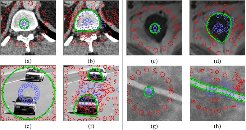
Figure 6 demonstrates our method with numerous im-ages. Starting with the upper left part of the figure, we show the segmentation of a CT image, where we would like to segment the bone in the center of the image. Placing some negative weighted constraints inside the bone, and positive constraints outside, we get an initial contour shown in (a). Using our method, we evolve the RBFs until convergence, producing the result shown in (b). In (c) we perform a sim-ilar experiment using a T1-weighted MR image of a lymph node, which appears as a darkish object in the center of the image. The converged result is shown in (d), which pro-vides an excellent segmentation of this object.

In (e) and (f) we present an example of a photographic image taken of a highway. Starting with an initial contour as depicted in (e), we evolve the RBFs until convergence, pro-ducing the result in (f). The segmentation is successful as it depicts the two cars; however, the result is not perfect as the Chan-Vese model we employ assumes that the image has a bimodal histogram with piece-wise constant regions, which is not the case for this image. A different image model, such as one based on non-parametric density estimation, would likely produce better results for this image. Any such curve evolution can be incorporated into our framework; however, this is left for future work. Also note that this example also demonstrates a topological split of the contour, which is needed to model the two separate objects. Finally, in (g) and (h) we show an example segmentation of a blood vessel from an angiography image. Starting with a small contour in the center, the contour grows outward along the vessel boundaries, providing an excellent segmentation result.

6. Conclusion

In this paper we presented a variational framework for evolving radial basis functions for active contour image seg-mentation. From an energy formulation, we derived

differ-ential equations for updating the RBF constraints so that they deform an active contour to achieve the segmenta-tion. From our derivation, we presented a simple way to evolve allof the parameters associated with the RBF, in-cluding the constraint centers, weights and anisotropy. The RBFs are not constrained to the contour location and only require minimal storage for evolution. We demonstrated the method’s effectiveness by segmenting several images.

For future work we are interested in implementing the method in 3D and comparing results obtained with differ-ent radial basis functions as well as differdiffer-ent functionals for image segmentation. Furthermore, we believe the theory underlying this paper will be useful in other applications, such as filtering, tracking, and registration; we plan on in-vestigating these topics in the future.

References

[1] V. Casselles, R. Kimmel, and G. Saprio. Geodesic Active Contours. The Intl. Journal of Computer Vision, 22(1):61– 79, 1997.

[2] T. Chan and L. Vese. Active Contours Without Edges.IEEE Trans. on Image Processing, 10(2):266–277, 2001.

[3] F. Chen and D. Suter. Multiple Order Laplacian Splines -Including Splines with Tension. Technical report, Monash University, Department of Electrical and Computer Systems Engineering, 1996.

[4] H. Q. Dinh, G. Turk, and G. Slabaugh. Reconstructing Sur-faces Using Anisotropic Basis Functions. InInternational Conference on Computer Vision (ICCV), pages 606–613, 2001.

[5] Y. Duan, L. Yang, H. Qin, and D. Samaras. Shape Re-construction from 3D and 2D Data Using PDE-Based De-formable Surfaces. InECCV, volume III, pages 238–251, 2004.

[6] H. Ho, Y. Chen, H. Liu, and P. Shi. Level Set Active Con-tours on Unstructured Point Clouds. InCVPR, pages 690– 697, 2005.

(a) (b) (c) (d)

Figure 5. Segmentation of an ultrasound image. In (a) through (d), we show the evolution of anisotropic RBFs at different time steps until convergence (d).

(a) (b) (c) (d)

(e) (f) (g) (h)

Figure 6. More examples. For each example, we show the initialization and the converged result. In (a) and (b): a CT bone image, (c) and (d): an MR lymph node image, (e) and (f): a photographic image of a highway, (g) and (h): an x-ray angiography image.

[8] J. Lachaud and J.Montanvert. Deformable Meshes with Au-tomated Topology Changes for Coarse-To-Fine 3D Surface Extraction.Medical Image Analysis, 3(2):187–207, 1999. [9] R. Malladi, J. Sethian, and B. Vemuri. Shape Modeling With

Front Propagation: A Level Set Approach. IEEE Trans. on Patt. Anal. and Machine Intelligence, 17(2):158–175, 1995. [10] T. McInerney and D. Terzopoulos. Topology Adaptive

De-formable Surfaces for Medical Image Volume Segmentation. IEEE Trans. on Medical Imaging, 18(10):840–850, 1999. [11] B. Morse, W. Liu, T. Yoo, and K. Subramanian. Active

Con-tours Using a Constraint-Based Implicit Representation. In CVPR, pages 285–292, 2005.

[12] M. Mullan, R. Whitaker, and J. Hart. Procedural Level Sets. InNSF/DARPA CARGO Meeting, 2004.

[13] D. Mumford and J. Shah. Optimal Approximation by Piece-wise Smooth Functions and Associated Variational Prob-lems.Commun. Pure Appl. Math, 42:577–685, 1989. [14] S. Osher and J. A. Sethian. Fronts Propagating

with Curvature-Dependent Speed: Algorithms Based on Hamilton–Jacobi Formulations. Journal of Computational Physics, 79:12–49, 1988.

[15] M. Rochery, I. Jermyn, and J. Zerubia. Higher Order Ac-tive Contours. International Journal of Computer Vision, 69(1):27–42, 2006.

[16] J. A. Sethian. Level Set Methods and Fast Marching Meth-ods Evolving Interfaces in Computational Geometry, Fluid Mechanics, Computer Vision, and Materials Science. Cam-bridge University Press, 1999.

[17] A. Tsai, A. Yezzi, and A. Willsky. Curve Evolution Im-plementation of the MumfordShah Functional for Image Segmentation, Denoising, Interpolation, and Magnification. IEEE Trans. Image Process., 10(8):1169–1186, 2001. [18] G. Turk and J. O’Brien. Shape Transformation using

Vari-ational Implicit Surfaces. InSIGGRAPH 99 Proceedings, pages 335–342, 1999.

[19] H. Wendland. Scattered Data Approximation. Cambridge Monographs on Applied and Computational Mathematics, 2005.