A low-complexity energy disaggregation method:
Performance and robustness
Hana Altrabalsi, Jing Liao, Lina Stankovic and Vladimir Stankovic
Department of Electronic and Electrical EngineeringUniversity of Strathclyde, Glasgow, G1 1XW, UK
Email:{h.altrabalsi, jing.liao, lina.stankovic, vladimir.stankovic}@strath.ac.uk.
Abstract—Disaggregating total household’s energy data down to individual appliances via non-intrusive appliance load mon-itoring (NALM) has generated renewed interest with ongoing large-scale smart meter deployments. Of special interest are NALM algorithms that are of low complexity and operate in real time, supporting emerging applications such as remote appliance scheduling and home automation, and use low sampling rates data from commercial smart meters. NALM methods, based on Hidden Markov Model (HMM) and its variations, have become the state of the art due to their high performance, but suffer from high computational cost. In this paper, we develop an alternative approach based on support vector machine (SVM) and k-means, where k-means is used to reduce the SVM training set size by identifying only the representative subset of the original dataset for the SVM training. The resulting scheme outperforms individual k-means and SVM classifiers and shows competitive performance to the state-of-the-art HMM-based NALM method with up to 45 times lower execution time.
I. INTRODUCTION
A large scale deployment of smart meters in households has started or it is about to start in many countries worldwide. For example, the UK Government has committed utilities to a roll out of automatic meter reading (AMR) systems by 2020. It is anticipated that by 2020 all UK households will be equipped with an AMR system that measures and displays in real time aggregate energy usage with an in-home display unit [1]. This large governmental investment promises significant improvements in energy demand via automatic, more efficient and more informed billing.
While the proposed acquisition, control, and communica-tions technologies have already been developed and agreed [1], it is still not clear how the massive amount of collected smart meter data will be utilized to ensure consumer-tailored and timely energy saving advice. One attractive solution is to provide appliance-itemized billing, which requires monitoring individual appliances, and could be more informative than current billing practices.
Since it is impractical to install and maintain individual load sensors for each and every appliance in a household, non-intrusive appliance load monitoring (NALM), i.e., disag-gregating individual appliance usage from the total, aggre-gated energy consumption captured at the energy monitor, is becoming increasingly popular. Besides appliance-itemized billing, NALM is useful to customers to determine which appliances are the most energy consuming ones, which are faulty, and when it is time to replace or service an old
appliance. NALM is also beneficial to suppliers to better plan power demand, to system operators to monitor the effect of smart grid fluctuations on the residential microgrid, to appliance manufacturers and policy makers.
NALM appeared in the research literature in 1980’s [2], and since then, many NALM algorithms have been proposed that improve the initial design of [2] and adapt to advances in sensor technology capturing energy measurands at a range of sampling rates, generally in the order of kHz. However, with large-scale smart metering deployment on the way, the increased interest is in NALM algorithms that work at lower sampling rates, in the order of seconds and minutes. It is not only the cost of the sensing technology [3], but also computational and storage cost as well as implementation efficiency that are key drivers towards the wide deployment of low-sampling smart meters. However, so far, there are no widely available efficient solutions for NALM, that offer high accuracy and low complexity at low sampling rates [4], [5].
Conventional event-based NALM algorithms consist of four steps. First, signal pre-processing is carried out, usually via data cleaning and filtering. Then, event detection is performed to isolate events when the state of an appliance has changed. After event detection, feature extraction is applied to isolate power features or signatures from the identified events, and finally, a classification method is used to classify extracted features into appliance groups. Many techniques have been applied to perform classification and optimization to design classifiers such as fuzzy logic, Naive Bayes, kNN, k-means, mean-shift, decision trees, neural networks, support vector machine, Hidden Markov Model, and many hybrid approaches (see [4]–[6] and references there in).
exponentially increases with the number of appliances, and the whole model needs to be retrained when a new appliance is added [5].
Another popular technique used for NALM is Support Vector Machine (SVM). SVM-based NALM has shown good performance especially for low frequency load features [5], it is scalable, and is a well established method for classifying noisy data. Non-linear classifiers, such as kernel SVM, that map the input feature space into a high dimensional space and find the optimal separating hyperplane between two classes to separate them, is one of the most effective classification methods, but has at least quadratic training time complexity. Thus, similarly to HMM, SVM-based approaches suffer from high computational complexity, due to necessary training on large scale data, which makes them unsuitable for real-time NALM applications.
The key problem of HMM-based and SVM-based ap-proaches is their high computational cost, that prevents their application for services that require real-time disaggregation, such as device scheduling, virtual power sensing, demand re-sponse capacity estimation, etc [6]. Motivated by increased de-mands for real-time NALM, we develop and analyze low-rate,
low-complexity NALM methods paying particular attention to
their applicability, in terms of running time, implementation issues and robustness to the size of the training set and training set labeling errors.
In particular, to benefit from high classification performance of non-linear SVMs and low computational cost of k-means clustering, we effectively combine conventional k-means and SVM obtaining a hybrid method that outperforms k-means and SVM classification alone. Inspired by [12]–[14], where k-means and SVMs are combined to reduce complexity, we use k-means to cleverly select a subset of input data used to train a linear SVM. By training the SVM only on a small set of representative samples, we are able to significantly reduce training and testing computational cost while demonstrating similar performance to that of the state-of-the-art HMM-based NALM approaches, which is demonstrated in the Section IV for 1min sampling rate and active power measurements only. The key contribution of this paper is:
• Novel real-time combined kmeans-SVM-based NALM
method for low sampling rate data;
• Innovative appliance-based selection of extracted features
that maximize performance;
• Experimental evaluation using different training sizes and
errors in labeling the training data;
• Comparison with state-of-the-art approaches using three
US households from the REDD data set [15].
The rest of the paper is organized as follows. Section II brings a brief background on NALM. Section III describes the proposed NALM algorithm. The last two sections discuss the simulation results, conclusion and future work.
II. BACKGROUND ANDLITERATUREREVIEW
Non-Intrusive Appliance Load Monitoring (NALM), also
referred to as NILM or NIALM [2], disaggregates total power
readings and identifies each appliance in use at any point in time based on the available measured total household consumption.
Traditional NALM methods consist of signal pre-processing, edge detection and feature extraction followed by classification. After acquisition, signal pre-processing can be done in the form of power normalization, filtering (for signal smoothing and getting rid of sudden peaks), and thresholding to remove small power loads that would appear as noise as well as the base-load, from appliances that are always running. Next, edge detection is done to identify events of appliances switching on and off. Edge detection is followed by extracting the features in the identified event windows. Classification is then used to group sets of extracted windows which have similar characteristics, such as power levels, time profile, reactive components etc.
In this paper, we focus on low complexity, low-rate NALM algorithms, where sampling rates are in the range of seconds and minutes. The sampling rate influences the type of features that can be used. For example, low-rate NALM approaches can use only steady-state parameters, such as active or real power [9], reactive power [2], [4], power factor [16], voltage or current waveform [17], [18].
The simplest approach, from an implementation point of view, is to use a current transformer (CT) sensor attached to the wire via a clump to measure alternating current and an AC-to-AC power adaptor with a circuit to measure voltage. This way, active and reactive power components can be calculated from the measured current and voltage. However, measuring voltage in a simple way requires additional plug points, which are often not available close to the electricity meter. Moreover, processing, communicating and storing two dimensional data (active and reactive power) is often impractical, especially because the reactive component is not needed for billing pur-poses. That is why, in this paper, we consider disaggregation using only active power values, obtained, for example, from the electric current measured via a simple CT sensor.
Based on the employed classification method, all NALM algorithms can be classified as supervised and non-supervised. Supervised NALM methods use labeled appliance events to train classifiers, and are usually based on optimization and pattern recognition approaches, such as rule-based, SVM or Bayes-based classification. Unsupervised methods do not re-quire labeled sets and are usually based on clustering [19] or HMMs [8]–[10].
disaggregates large loads such as air conditioners using very low granularity measurements, sampled every 15 mins, and extracting features such as occurrence, timing and magnitude of all large changes. Other NALM work for disaggregating large loads include [22], [23], and [24].
Recent work on NALM is mainly focused on state-based probabilistic methods. In [8] four different methods for low-rate NALM are proposed using (conditional) factorial HMM and Hidden semi-Markov models. The obtained accuracy was in the range between 72% and 99% for 3sec sampling rate in seven different houses with up to 10 appliances with an average accuracy of 83%. This method cannot disaggregate base load, such as, for example, refrigerator, it is not of low computational complexity, and is prone to converge to a local minimum.
In [9] a factorial HMM is used for disaggregation of active power load at 1min sampling rate. The method uses expert knowledge to set initial models for states of known appliances. To obtain reliable results, it is necessary to correctly set the a priori-values for each state for each appliance, which in turn is strongly dependent on the particular aggregate dataset on which NALM is being performed. Indeed, a similar factorial HMM-based approach is tested in [15], where it is shown that the disaggregation accuracy drops by up to 25% when different houses are used to set the initial models compared to the case when the same house is used for building the models (training) and testing. Results are reported for REDD dataset [15] with sampling rates of 1sec and 3sec.
In [19], [25], and [26] a decision-tree (DT) classifier is used for pattern matching. The DT-based algorithm developed in [25], is a low-complexity, supervised approach that uses only rising and falling active power edges to build a DT model that is used for classification. The method is not scalable, since re-training is needed whenever a new appliance is added, but is fast and performs well even when the training period is very short.
In [10], an unsupervised Additive Factorial Approximate Maximum A-Posteriori (AFMAP) inference algorithm is pro-posed using differential factorial HMMs. First, all snippets of active power data are extracted using a threshold and modelled by an HMM; next the k-nearest-neighbor graph is used to build nine motifs that are treated as HMMs over which AFMAP is run. The results show average accuracy of 87.2% using 7 appliances and sampling rate of 60Hz. In [11] Hierarchical Dirichlet Process Hidden Semi-Markov Model (HDP-HSMM) factorial structure is used removing some limitations of the approach of [8] at increased complexity. The results are reported for five devices using 20sec resolution with 18 24-hour segments across four houses from the REDD dataset [15] obtaining disaggregation accuracy of 81% outperforming the EM-based method of [15].
The main problem with the above state-based approaches is that they are not suitable for real-time applications due to their high computational complexity. See, for example, [6] for some examples. The low-complexity HMM-based method proposed in [27] reduced execution time 72.7 times, but still requires
11.4 seconds for disaggregating two appliances using 524,544 readings or 94 minutes for 11 appliances.
III. PROPOSED LOW-COMPLEXITYNALM
In this section, we describe the proposed NALM method. First, we discuss pre-classification steps. Then, we show that trained k-means and SVM-based classification alone are not suitable for real-time NALM application, either due to modest performance or high execution time. Finally, we propose a combined k-means/SVM classification method using different extracted power features.
The algorithm comprises two phases: a training phase and a testing phase. Training is always done on aggregate data using a labeled dataset, which is obtained from time-diaries or sub-metering. The entire disaggregation procedure includes three steps: event detection, feature extraction, and classification. In the proposed solution we use the efficient edge detection method of [25] and focus on improving the feature extraction and classification steps. In the following, we closely follow the notion of [25], which we review next.
Let M be a set of all known appliances in the house. Let p(ti) be active power measured at time instance ti. Without loss of generality, in the following we denotep(ti)asp(ti) =
p(iT) =p(i), where T =ti−ti−1 is the sampling interval.
The disaggregation task is to find pj(i)for allj, such that p(i) =PMj=1pj(i) +n(i), where pj(i)≥0 is the power load
of appliance j andn(i) is the measurement noise. Note that pj(i)is zero if the appliance is off at time instanceiT.
A. Event Detection and Feature Extraction
The task of the event detection is to detect changes in time-series aggregate load curve due to one or more appliance being switched on/off or changing its state. LetW be a set threshold. Then, if |pj(i)−pj(i−1)| ≥ W then the appliance j has
changed state at time instantiT.
Threshold W needs to be set low enough so that for all j, if |pj(i) − pj(i − 1)| ≤ W Appliance j did not change its state and, otherwise, it did change its state. W depends on the set of appliances being monitored, and is adapted automatically during the training process based on the minimum state transition that needs to be detected and the maximum variation of the active power within one appliance state across all appliances’ states, that is
W = max{min
m∈M
pm,max
m∈M|max(
pm)−min(pm)|}, (1) where pm is a vector of active power readings of appliance m. Note that the value ofW depends on the set of available appliances, and is adaptively changed as appliances are being disaggregated and removed from the aggregate load.
An event occurs whenever an appliance changes its state. Edge detection is used to detect events by comparing|p(i)− p(i−1)| with W. We say a window of the event started at timels and ended atleif an appliance changed its state at ls andle, and
where C is parameter smaller than W.
Next, from each detected event window, features are ex-tracted and stored. Exex-tracted features could be simply all active power readings in the event window, or only rising/falling edge, or maximum/minimum value, area, etc.
B. Classification
Extracted features from each detected event are matched to the pre-defined appliance classes using a trained classifier. First, we test two conventional techniques to perform classifi-cation and pattern matching: trained k-means and SVM.
Trained k-means uses the labeled dataset to find the optimal cluster heads and cluster distribution. The number of clusters is always set to the number of known appliances in the household. The aggregate load is then grouped into known appliance subsets and the centroid of each subset is set as cluster head. When a new testing sample (feature vector -active power load) is introduced, it is compared to all cluster heads, and the minimum distance determines the classification outcome.
SVM-based algorithms are optimal classifiers in the pres-ence of noise and proven to perform well for NALM ap-plications [5]. We train binary classifiers to separate one appliance at the time. After an appliance has been classified, its contribution is removed, the thresholdW in (1) is adapted, and the next appliance is considered.
As will be shown in the next section, while the trained k-means-based NALM is time efficient, it provides low dis-aggregation performance. On the other hand, the SVM-based NALM method significantly outperforms the trained k-means-based approach, but requires up to 10 times more computa-tional time.
In order to design a high-performance, low-complexity solution, we propose to use a linear SVM on a substantially reduced training set obtained using means. Combining k-means and SVM has been studied before, but not in the context of NALM. Recognizing that in a majority of cases a large portion of the input data is redundant for training, in [28], k-means is used to decrease the number of support vectors and the training set size. Similarly, in [12], [13], k-means is employed to select a subset of original data for the SVM training. In [14], a clustered SVM is proposed that, in a divide-and-conquer manner, trains a linear SVM on each of the k-means clusters.
To combine k-means and SVM, we first train k-means as explained above using the entire original dataset. As a result,k clusters each corresponding to one appliance are formed with a centroid as cluster head. All feature vectors falling in Clusteri that are at an Euclidian distance larger thanrfrom their cluster head, form a subset Ci that is used to train a linear SVM for Appliancei.ris a pre-set threshold, obtained heuristically, that is used to tradeoff complexity and performance. Algorithm 1 shows the training steps, where d(x, y)denotes the Euclidian distance between vectors xandy.
During testing, if the Euclidian distance between a tested sample and any cluster head is smaller than a pre-set threshold,
Algorithm 1 Training: Perform training on the extracted
features of the collected dataset L. function TRAIN(L,|M|)
k=|M| ⊲Number of Appliances [Cluster,c]=kmeans(k, L)
⊲ReturnsClusterdistribution and cluster headsc.
fori= 1 :kdo Ci={∅}
For∀l∈Clusterido
ifd(l, ci)≥r then Ci=CiS{l}
end if
SV M T rain(Ci) end for
end function
then the sample is classified to the closest cluster head using the trained k-means. Otherwise, the sample is input to the SVM classifier. The proposed combined method has low execution time, since many samples are going to be classified rapidly using k-means, and has good performance, since SVM improves classification for samples that would most likely be incorrectly classified using the trained k-means.
IV. RESULTS ANDDISCUSSION
In this section we present our experimental results and discuss our main findings. We use House 1, House 2 and House 6 from the publicly available REDD database [15] downsampled to 1min resolution. The training size was varied in the experiments, and testing is always performed on four weeks worth of data.
The evaluation metrics used are precision (PR), recall (RE) and F-Measure (FM) [29] defined as:
P R=T P/(T P +F P) (2)
RE=T P/(T P +F N) (3)
FM = 2∗(P R∗RE)/(P R+RE), (4) where true positive (TP) presents the correct claim the detected event was triggered by the use of the appliance, false positive (FP) represents an incorrect claim that an appliance triggered the detected event, and false negative (FN) indicates that the appliance used was not identified.
TABLE I
COMPARISON BETWEEN THE THREE METHODS USINGFMANDEXECUTION TIME USINGREDD HOUSE1.
SVM k-means Combined method
Features train(sec) test(sec) FM(%) train(sec) test(sec) FM(%) train(sec) test(sec) FM(%)
Max and duration 0.74 0.69 71.3 0.17 0.17 70.6 0.36 0.10 75.94
Max and Max/mean 0.82 0.60 76.1 0.17 0.17 70.2 0.32 0.05 73.1
Max, area and Max/mean 1.12 0.67 70.7 0.26 0.26 65.1 0.36 0.45 53.3
Min, area and Max/mean 1.29 0.7 68.8 0.19 0.19 68.7 0.56 0.41 69.6
for the best two 2D and two 3D classifiers. The results are averaged over all known appliances.
It can be seen from Table I that the SVM-based method always outperforms the trained k-means, but requires more time for both training and testing. The best SVM-based NALM result is obtained for the 2D classifier using maximum and maximum/mean factor and performs 6% better than the best k-means-based performance, but is more than 4 and 3 times slower when performing training and testing, respectively. The combined approach provides a good tradeoff reducing the training and testing time by over 2 and 6 times, respectively, compared to the SVM-based method.
Interestingly, the selection of features has a significant impact on the performance. For example, using an area as a feature together with maximum/mean factor and maximum or minimum does not lead to good results. The best com-bined method is only 0.15% worse than the best SVM-based approach, but reduces the execution time by over three times. Table II shows results per appliance for the combined method. Marked with bold typeface are the best features for each appliance. All features denote the 5D case, where max, min, max/mean, duration and area are used. One can see that for different appliances different features give the best performance. For example, only 5D classification gives non-zero disaggregation for the toaster. Since we are classifying one appliance at a time, it is possible to adapt classification features from appliance to appliance. Thus, during the training, the best features to use are identified per appliance which are then used during testing. In the following, we refer to this method, as theproposed combined method.
Table III shows the obtained results for all known appliances in House 2. In House 2, there are five known appliances listed in the first column of the table. All other appliances are considered unknown. We compare the proposed approach with the state-of-the art HMM-based method of [9], which was designed for low-sampling (1 min) rates. For each dataset, all three tested algorithms always use the same amount of data for training (7000 samples or roughly one week) and testing (four weeks). The HMM-based method [9] requires prior initialization of the model using expert knowledge (state variances, mean value for each state and state transition probabilities), which was carried out in our experiments either using the information provided by the authors of [9], or were
2000 3000 4000 5000 6000 7000
65 70 75 80 85 90 95 100
Training Size
F−measure (%)
HMM−H1 Proposed−H1 HMM−H2 Proposed−H2 HMM−H6 Proposed−H6
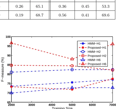
Fig. 1. Effect of varying the training size on the performance of the two NALM methods for the three REDD houses.
generated during training. The SVM-based method selects the best features to use for each appliance and then performs SVM-based classification.
It can be seen from the table that the proposed method out-performs the HMM-based approach for all appliances except the stove, which was often confused for the refrigerator, and microwave, for which SVM shows poor result. The proposed algorithm is always better than the SVM-based approach. All three algorithms struggle with the dish washer, but show very good results for the refrigerator, which was always on, so the number of event samples for training was the largest.
Table IV shows the average results for all three tested houses. It can be seen that the proposed method provides the same or better performance than HMM, while its execution time (including training and testing) is up to 240 times less. The SVM-based method requires more time than the proposed method and provides similar performance.
[image:5.595.323.552.199.415.2]TABLE II
FMRESULTS FOR THE COMBINED METHOD FOR DIFFERENT APPLIANCES AND DIFFERENT EXTRACTED FEATURES USINGREDDHOUSE1.
FM(%)
Features Ref rigerator M icrowave T oaster DishW asher W asherDryer
Max and area 89.49 20.7 0 28.7 53.7
Max, Min and Max/mean 85.68 63 0 7.27 40.75
All features 84.51 15.38 4.76 11.76 57.53
Min and Max/mean 83.35 16.21 0 35.97 29.16
Max and Duration 88.51 56 0 32.5 75.36
TABLE III
COMPARISON BETWEEN THE THREENALMMETHODS USINGREDD HOUSE2.
PR(%) RE(%) FM(%)
Appliances HM M SV M P roposed HM M SV M P roposed HM M SV M P roposed
Refrigerator 87.45 93.41 92.87 87.93 91.76 95.88 87.69 92.58 94.35
Stove 38.10 4.1 66.6 66.67 33.3 33.3 48.48 7.4 44.4
Microwave 35.71 0 15.38 58.14 0 82.05 44.25 0 25.91
Toaster 54.9 54.9 69.6 92.45 93.3 91.66 64.90 69.1 79.13
Dish Washer 33.33 33.3 22.22 7.56 21.42 42.85 12.32 26.08 29.2
TABLE IV
COMPARISON BETWEEN THE THREENALMMETHODS FOR THE THREEREDDHOUSES. ALL RESULTS ARE AVERAGED OVER ALL KNOWN APPLIANCES.
HMM SVM Proposed method
House P R(%) RE(%) FM(%) T ime(sec) P R(%) RE(%) FM(%) T ime(sec) P R(%) RE(%) FM(%) T ime(sec)
House 1 77.16 76.97 77.06 51.22 80.3 80.3 80.3 1.55 78.66 76.42 77.52 1.13
House 2 84.85 80.05 82.38 40.86 85.18 85.92 85.55 1.94 73.3 93.4 82.17 0.8
House 6 58.64 96.32 72.76 46.41 72.85 90.4 80.68 1.22 95.09 96.07 95.58 0.19
appliance is not operating alone, model generation will not be successful. Drop in the performance of the HMM as the size of the training set is reduced, is due to the fact that more appliances are not modeled properly and hence are not disaggregated. The training execution time of the proposed method slightly increases as the training set size increases but it is still significantly lower than that of the HMM-based approach for all houses and all training sizes. Indeed, the proposed method needs 32-88 and 1.43-3 times less time for testing than HMM and SVM, respectively, and 40.45-274 and 1.18-6.27 times less time for training than HMM and SVM, respectively.
Table VII present results when random labeling errors are introduced during the training process. For example, 5% means that every fifth event of one hundred events was randomly labeled during training. Note that it is possible for FM to slightly increase if the number of errors increase due to the
decrease in FN and FP. One can see that both methods show robustness to errors in the training dataset.
V. CONCLUSION
In this paper we proposed a low-complexity approach for energy disaggregation based on k-means clustering and Support Vector Machine (SVM). Experimental results using REDD data demonstrate the potential of the proposed solu-tions. Indeed, the proposed approach shows similar perfor-mance to that of HMM, with up to 88 and 274 times lower execution time for testing and training, respectively. Tests, con-ducted by reducing the training size and introducing errors in the training data, showed robustness of the proposed approach, that is capable of performing successful disaggregation using only two days of training data and up to 20% of errors in the training set.
TABLE V
EXECUTION TIME[SEC]FOR THE THREEREDDHOUSES USING THREE DIFFERENT TRAINING SIZES.
HMM k-means SVM Proposed method
House trainingsize train test train test train test train test
2000 15.18 21.29 0.18 0.18 0.37 0.57 0.19 0.32
House 1 5000 23.79 19.27 0.25 0.25 0.76 0.65 0.27 0.25
7000 28.32 22.90 0.2 0.2 0.83 0.78 0.7 0.26
2000 18.38 18.56 0.09 0.25 0.43 0.72 0.1 0.32
House 2 5000 21.13 18.03 0.06 0.2 0.84 0.72 0.3 0.34
7000 22.77 18.09 0.23 0.23 1.15 0.79 0.25 0.55
2000 20.52 10.99 0.07 0.18 0.33 0.35 0.12 0.2
House 6 5000 22.46 13.91 0.09 0.14 0.56 0.45 0.15 0.26
7000 30.22 16.19 0.24 0.24 0.69 0.53 0.11 0.28
TABLE VI
F-MEASURE(%)FOR THE TWONALMMETHODS FOR THEREDD HOUSE2USING THREE DIFFERENT TRAINING SIZES.
HMM Proposed combined method
Appliances 7000 5000 2000 7000 5000 2000
Refrigerator 87.69 83.42 83.55 94.35 91.88 90.22
Microwave 44.25 44.25 44.25 25.91 0 0
Dish Washer 12.32 12.32 0 29 0 0
Toaster 64.90 64.90 0 79.13 17.1 60
Stove 48.48 0 0 44.4 0 0
TABLE VII
F-MEASURE(%)FOR THE TWONALMMETHODS FOR THEREDD HOUSE2WHEN ERRORS ARE INTRODUCED IN THE TRAINING SET DATA.
HMM Proposed combined method
Appliances 0% 5% 15% 20% 0% 5% 15% 20%
Refrigerator 87.69 83.42 83.42 83.55 94.35 91.88 93.32 91.9
Microwave 44.25 44.25 44.25 0 25.91 0 0 0
Dish Washer 12.32 12.32 12.32 12.32 29.2 28.57 33.33 21.4
Toaster 64.90 64.90 46.97 46.97 79.13 11.42 11.94 8.9
Stove 48.48 48.48 18.65 18.65 44.4 0 0.00 0.00
real-time applications of NALM for emerging services such as home automation and intelligent appliance scheduling as well as forming home area networks of virtual power sensor nodes facilitating demand side management. A downside of the proposed approach is that it requires re-training whenever a new appliance is introduced. A part of the future work is developing efficient training methods and detailed evaluation
of the system in a real-world environment.
ACKNOWLEDGMENT
Innovation (BuildTEDDI) funding programme. The authors would like to thank O. Parson for sharing his code, and J. Kolter and M. Johnson for making the REDD database available.
REFERENCES
[1] Government response to the consultation on the second version of the Smart Metering Equipment Technical Specifications: Part 2, Department of Energy & Climate Change UK, December 2013.
[2] G. W. Hart, “Nonintrusive Appliance Load Data Acquisition Method”, MIT Energy Laboratory Technical Report, Sept. 1984.
[3] K.C. Armel, A. Gupta, G. Shrimali, and A. Albert, “Is disaggregation the holy grail of energy efficiency? The case of electricity,” Energy Policy, vol. 52, pp. 213–234, 2013.
[4] M. Zeifman and K. Roth, “Nonintrusive appliance load monitoring: Review and outlook,” IEEE Trans. Consumer Electronics, vol. 57, no. 1, pp. 76–84, Feb. 2011.
[5] A. Zoha, A. Gluhak, M.A. Imran, and S. Rajasegarar, “Non-intrusive load monitoring approaches for disaggregated energy sensing: A survey,” Sensors, vol. 12, pp. 16838–16866, Dec. 2012.
[6] S. Barker, S. Kalra, D. Irwin, and P. Shenoy, ”NILM redux: The case for emphasizing applications over accuracy,” NILM-2014 Workshop, Austin, TX, June 2014.
[7] T. Zia, D. Bruckner, and A. Zaidi, “A Hidden Markov Model based procedure for identifying household electric loads,” In Proc. IECON-2011 37th Annual Conf. IEEE Industrial Electronics Society, Melbourne, Australia, Nov. 2011.
[8] H. Kim, M. Marwah, M. Arlitt, G. Lyon, and J. Han, “Unsupervised disaggregation of low frequency power measurements,” in Proc. 11th SIAM Int. Conf. Data Mining, Mesa, AZ, April 2011.
[9] O. Parson, S. Ghosh, M. Weal, and A. Rogers, “Non-intrusive load monitoring using prior models of general appliance types,” in Proc. the 26th Conf. Artificial Intelligence (AAAI-12), Toronto, CA, pp. 356–362, July 2012.
[10] J. Kolter, and T. Jaakkola, “Approximate inference in additive factorial HMMs with application to energy disaggregation,” in J. Machine Learning, vol. 22, pp. 1472–1482, 2012.
[11] M.J. Johnson and A.S. Willsky, “Bayesian nonparametric Hidden Semi-Markov Models,” J. Machine Learning Research (JMLR), vol. 14, pp. 673701, Feb. 2013.
[12] J. Wang, X. Wu, and C. Zhang, ”Support vector machines based on K-means clustering for real-time business intelligence systems,” Int. J. Business Intelligence and Data Mining, vol. 1, no. 1, pp.54-64, 2005. [13] Y. Yao, Y. Liu, Y. Yu, H. Xu, W. Lv, Z. Li, and X. Chen, ”K-SVM: An
Effective SVM Algorithm Based on K-means Clustering,” J. Computers, vol. 8, Oct. 2013.
[14] Q. Gu and J. Jan, ”Clustered Support Vector Machines,” in Proc. AISTATS-2013 16th Int. Conf. Artifical Intelligenece and Statistics, Scotts-dale, AZ, 2013.
[15] J. Kolter, and M. Johnson, “REDD: A public data set for energy disaggregation research,” in Workshop on Data Mining Applications in Sustainability (SIGKDD), San Diego, CA, 2011.
[16] A. G. Ruzzelli, C. Nicolas, A. Schoofs, and G.M.P. O’Hare, “Real-time recognition and profiling of appliances through a single electricity sensor, ”IEEE SECON-2010 7th Annual Conf. Sensor Mesh and Ad Hoc Communications and Networks , pp.1–9, Boston, June 2010.
[17] C. Laughman, K. Lee, R. Cox, S. Shaw, S. Leeb, L. Norford, and P. Armstrong, “Power signature analysis,” IEEE Power and Energy Magazine, vol. 1, pp 56–63, Mar-Apr 2003.
[18] J. Liang, S. K. K. Ng, G. Kendall, J. W. M. Cheng, “Load signature study part I: Basic concept, structure, and methodology,” IEEE Trans. Power Delivery, vol. 25, no. 2, pp. 551–560, Apr. 2010.
[19] M. Berges, E. Goldman, H. S. Matthews, and L. Soibelman, “Learning systems for electric consumption of buildings,” in Proc. 2009 ASCE Int. Workshop Computing in Civil Engineering, Austin, TX, 2009. [20] Electric Power Research Institute, Low-cost NIALMS technology.
Elec-tric Power Research Institute, Technical Report TR-198918-V1, Sept. 1997.
[21] J. Powers, B. Margossian, B. Smith, “Using a rule-based algorithm to disaggregate end-use load profiles from premise-level data,” IEEE Computer Applications in Power, vol. 4, no. 2, pp. 42–47, 1991.
[22] L. Farinaccio and R. Zmeureanu, “Using a pattern recognition approach to disaggregate the total electricity consumption in a house into the major end-uses,” Energy & Building, vol.30, pp. 245–259, 1999.
[23] M. L. Marceau and R. Zmeureanu., “Nonintrusive load disaggregation computer program to estimate the energy consumption of major end uses in residential buildings,” Energy Conversion & Management, vol. 41, pp. 1389–1403, 2000.
[24] M. Baranski and J. Voss, “Genetic algorithm for pattern detection in NIALM systems,” in Proc. SMC-2004 IEEE Int. Conf. Sys., Man and Cybernetics, pp. 3462-3468, Hague, Netherlands, Oct. 2004.
[25] J. Liao, G. Elafoudi, L. Stankovic, and V. Stankovic, ”Power disaggrega-tion for low-sampling rate data,” 2nd Int. Non-intrusive Appliance Load Monitoring Workshop, Austin, TX, June 2014.
[26] J. Liao, G. Elafoudi, L. Stankovic, and V. Stankovic, “Non-intrusive appliance load monitoring using low-resolution smart meter data,” Smart-GridComm IEEE International Conference on Smart Grid Communica-tions, Venice, Italy, November 2014.
[27] S. Markonin, I.V. Bajic, and F. Popowich, ”Efficient sparse matric processing for nonintrusive load monitoring,” 2nd Int. Non-intrusive Appliance Load Monitoring Workshop, Austin, TX, June 2014. [28] X.L. Xia, M.R. Lyu, T.M. Lok, and G.B. Huang, ”Methods of decreasing
the number of support vectors via k-mean clustering,” in ICIC 2005, LNCS 3644, pp. 717–726, Spinger-Verlag Berlin Heidelberg, 2005. [29] D.L. Olson and D. Delen, Advanced Data Mining Techniques, Springer,