Multiple depth maps integration for 3D reconstruction using geodesic graph cuts

Multiple Depth Maps Integration for 3D

Reconstruction using Geodesic Graph Cuts

Jiangbin Zheng

1

_{, Xinxin Zuo}

1

_{, Jinchang Ren}

2

_{, Sen Wang}

3

1_{Shaanxi Provincial Key Laboratory of Speechand Image Information Processing, Schoolof Computer,} Northwestern Polytechnical University, Xi’an, P.R, China

2

Dept. of Electronic and Electrical Engineering, University of Strathclyde Glasgow, G1 1XW, United Kingdom 3_{School of Mechanical Engineering, Northwestern Polytechnical University, Xi’an, P.R, China}

Email: [email protected], [email protected], [email protected]

Abstract

Depth images, in particular depth maps estimated from stereo vision, may have a substantial amount of outliers and result in inaccurate 3D modelling and reconstruction. To address this challenging issue, in this paper, a graph-cut based multiple depth maps integration approach is proposed to obtain smooth and watertight surfaces. First, confidence maps for the depth images are estimated to suppress noise, based on which reliable patches covering the object surface are determined. These patches are then exploited to estimate the path weight for 3D geodesic distance computation, where an adaptive regional term is introduced to deal with the “shorter-cuts” problem caused by the effect of the minimal surface bias. Finally, the adaptive regional term and the boundary term constructed using patches are combined in the graph-cut framework for more accurate and smoother 3D modelling. We demonstrate the superior performance of our algorithm on the well-known Middlebury multi-view database and additionally on real-world multiple depth images captured by Kinect. The experimental results have shown that our method is able to preserve the object protrusions and details while maintaining surface smoothness.

Keywords

Multiple depth maps integration; Geodesic distance; Adaptive regional term; Graph cuts

1. Introduction

With increasing availability of consumer depth cameras that enable 2.5D measurements of real-world surfaces, quite a few approaches were developed to reconstruct full 3D models from such 2.5D range data, especially using multi-view stereo (MVS) reconstruction [1-3]. Due to a substantial amount of outliers contained in the acquired depth images, in particular depth maps estimated from stereo vision, this may have, as a challenging issue, severely affected the quality of the 3D models reconstructed from multiple depth images. As a result, a certain level of regularization is required to obtain smoother surfaces, where a number of techniques have been proposed as discussed below.

The fundamental of robust depth image fusion in the context of laser scanned data was proposed by Curless and Levoy [4]. Using an intermediate volumetric representation allows the generation of models with arbitrary genus and avoids the numerical difficulties encountered with polygonal techniques [5]. As pointed out in [6], simple averaging without further regularization causes inconsistent surfaces due to frequent sign changes of the mean distance field. Therefore, an additional regularization force is required to favor smooth geometry. The smoothness of the obtained surface is enforced implicitly in minimal surface based energy function. Graph-cut algorithms [7-9] and variational techniques [10,11] are exploited to determine the optimal surface under a given energy function. Moreover, Zach et al. [6] proposed an efficient numerical scheme to incorporate a total variation regularization term with a L1 data fidelity term for energy minimization.

adjusted according to photo-consistency in multiple color images using bundle optimization. Finally, the mesh model is generated using Delaunay or Poisson meshing methods [15]. However, this kind of approach is not appropriate for integration of depth maps obtained from quite sparse viewpoints.

For 3D MVS reconstruction, one commonly used approach is to embed a graph into a volume containing the surface and estimate the surface as a cut separating free-space (exterior) from the interior of the object or objects [1-2], and the cut cost corresponds to the energy of minimal weighted surface. After the early work by Vogiatzis et al. [1], graph cuts based 3D reconstruction has been exploited in several recent works [2,3,18]. However, conventional graph-cuts based MVS reconstruction approaches suffer from an inherent and well-known bias towards shorter cuts, which is caused by a summation over the surface of the reconstructing object contained in the minimized energy function. As a result, thin or protrusive parts of the reconstructed object surface were cut off, as shown in Fig. 1(b). Previous works related to reducing such bias include introducing additional silhouette constraints [19], constant or data-aware ballooning term [20], and iterative graph-cut over narrow bands combined with an accurate surface normal estimation [21].

In this paper, we exploit the graph-cut based energy minimization method for depth maps fusion which has shown its success in multi-view reconstruction. By integrating a defined 3D geodesic-distance to the energy function, an adaptive regional term or ballooning term is obtained. The inspiration of our approach comes from the fact that geodesic segmentation [22], a widespread seed-expansion method for 2D image segmentation, can robustly segment long, thin structures without regard to boundary length. As shown in Fig. 1(c), our proposed algorithm can significantly reduce overcarving problems and preserves protrusions of the surface. Also, to be different from the traditional graph-cut based MVS method, an extra initial bounding volume or visual hull is no longer needed in our approach. Detailed discussions of the proposed method and experimental results are presented in the next several sections. It is shown that we are able to get 3D watertight models from even sparse and noise contaminated depth maps obtained with both passive and active methods.

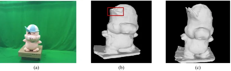
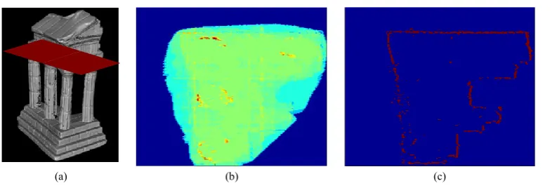
[image:2.595.116.493.372.488.2]

(a) (b) (c)

Figure 1. Shorter-cuts problems. (a) shows the color image captured using Kinect. (b) is the reconstruction result using standard graph-cuts methods. (c) gives the mesh model reconstructed using the proposed approach. The experimental details are demonstrated in the experimental part.

In addition, patch-based representation is exploited in this paper with patches embedded into the evenly divided voxels so as to generate the patches more efficiently and get them stored in a more compact way while taking advantages of patches in photo-consistency computation. The patch-based representation has gained its big success in multi-view reconstruction [16,17]. Compared with the voxels often used in volumetric graph cuts, the patches have shown to be more flexible and robust for photo-consistency computation considering the distortion of surface projection in multiple images, especially in object areas with high curvature. Also, the patches can be naturally integrated to the graph structure as pointed out in [16].

2. Overview of the Proposed Approach

patches before reaching the background space (outside). Finally, the geodesic distance based regional term and the photo-consistency based boundary term are combined in the graph cut framework, as shown in Eq. (1),

( ) ( ) ( )

S V

E S 





x dA







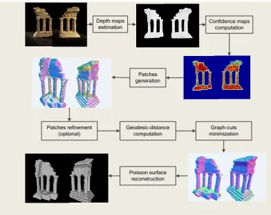
x dV (1) Eq(1) gives the energy function where the first term is the boundary term and the second term is our proposed adaptive regional term. The boundary term is affected by photo-consistency of corresponding color images and it is supposed that the reconstructed surface has overall minimized photo-consistency cost. The over smoothing problem arises because of the summation over the surface of the reconstructing object. The adaptive regional term is constructed by patches covering the underlying surface and forces the voxels inside surface to be labeled as strong inside so as to decline over carving affect.

To illustrate how the proposed approach works, a diagram of the framework is given in Fig. 2. First, the depth maps are estimated from multiple color images using stereo method, followed by confidence maps computed for each depth image, which can be integrated into the fusion procedure to suppress depth noise. These are discussed in detail in Section 3. Second, patches covering the surface are generated and optionally refined using photo-consistency as presented in Section 4. Third, we compute 3D geodesic distance for every voxels in the space according to the reliable patches, as given in Section 5, which is defined as an adaptive regional term to be fused to the graph-cut minimization framework. Finally, 3D points derived from graph-cut energy minimization are further processed to construct mesh model using Poisson Surface Reconstruction method, as detailed in Section 6. To verify the effectiveness of the proposed approach, experimental results are presented in Section 7 with some concluding remarks drawn in Section 8.

Depth maps

estimation Confidence maps computation

Patches generation

Patches refinement (optional)

Geodesic-distance computation

Graph-cuts minimization

[image:3.595.102.495.343.654.2]

Poisson surface reconstruction

Figure 2.The framework of our reconstruction algorithm.

Each depth image demonstrates the reconstruction results for an object from one particular viewpoint. According to the capturing device, the existing depth acquisition approaches can be divided into two categories, i.e. passive methods based on stereo matching of multiple color images and active methods based on structured light or time-of-flight, respectively.

3.1 Depth image estimation

In our approach, given multiple color images, we obtain the multi-view depth maps using the depth estimation approach proposed by Campbell et al [3], which stores multiple depth hypotheses and use a spatial consistency constraint to extract the true depth. This approach is adopted as it can demonstrate robustness to spurious matches caused by repeated texture and matching failure due to occlusion, distortion and lack of texture [23].

In addition, our depth integration method is also verified on multiple depth images captured using Kinect. There exists non-negligible noise in the acquired depth image due to inherent problems of consumer cameras: optical noise, loss of depth information on the shiny surfaces and occlusion areas, and also flickering artifacts [24]. As a result, the originally captured depth images are smoothed using our refined weight mode filtering method as proposed in paper [25] before being used in the integration procedure.

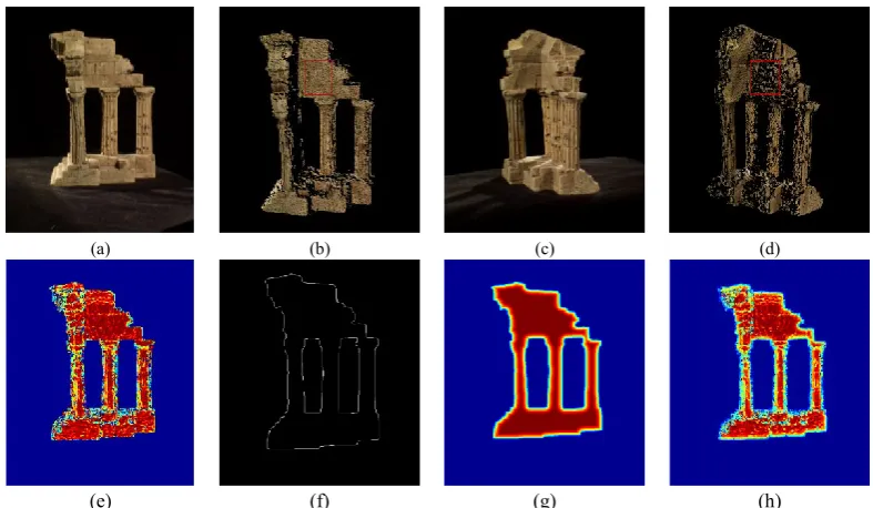
As what can be seen from the depth images estimated using passive stereo or captured with active depth cameras (e.g. Kinect), the depth maps generated from different viewpoints give various accuracy for particular part of the reconstructing object, as shown in Figure 3(a-d). To be more concrete, the depth image is of the highest accuracy when the spindle of the corresponding camera is nearly parallel to the particular part of the object surface. In addition, the depth value for pixels around the boundary of the object contains much noise, which is caused by occlusion in that area. Taking these issues into consideration, it is necessary to define confidence maps for depth images, which can be used to integrate multiple depth images to obtain a watertight 3D model. With the confidence map, we can suppress the influence of the error existed in the depth image on the final model.

(a) (b) (c) (d)

[image:4.595.100.494.395.624.2]

(e) (f) (g) (h)

Figure 3.Confidence maps for depth images: (a) and (c) are images from different viewpoints, and (b)(d) displays the estimated depth images rendered in 3D; The particular object parts (highlighted with red boxes) exhibition quite different accuracy for depth images generated from different viewpoints; (e) and (g) gives the confidence maps generated using normal and boundary constraints for depth image(b), respectively; and (h) shows the confidence maps computed with these two kinds of constraints.

3.2 Confidence maps computation

constraints and object boundary constraints, which are constructed using the angle between the viewpoint direction and surface normal, and the distance from the object boundary, respectively.

(1) Surface normal constraints

First, we need to determine the surface normalnormal p( )0 for every pixelp0in the depth image. As the

actual surface is unknown, the surface normal is estimated using its neighboring pixelsN p( )0 . To be more

specific, the neighboring pixels satisfying the following constraints (Eq. (2)) are back projected to the camera coordinate using the camera parameters. Afterwards, Principal Component Analysis (PCA) is performed on the covariance of these 3D points. Three Eigenvalues(

 

1 2



3), representing the weights of the corresponding directions of the Eigenvectors( , , )v v v1 2 3 , are obtained by decomposition of the covariance matrix. The Eigenvector

v

3corresponding to the smallest Eigenvalue is selected as the estimated surface normal.

~

0 0 0

( ) { ( ) | ( ) ( ) }

N p  q N p D p D q Thres (2)

Then, the normal confidence for the pixelp0is computed as the inner product of the surface normal

0

( )

normal p and its viewpoint directionview p( )0 .

0 0 0

_ ( ) ( ) ( )

conf normal p view p normal p (3)

(2) Object boundary constraints

First, given the silhouette of the object, the canny edge detector [26] is utilized to extract the boundary of the object. As shown in Fig. 3(f), the pixels on the edge have value 1, denoted asedgeset. For every particular pixelp0in the image, the nearest distance fromp0to pixels in theedgeset is computed as:

0 _{q edge}min 0

d p q



  (4)

To get reasonable confidence map with the distance, we exploit the sigmoid function to convert the distance to confidence value ranging 0~1:

0

0

1

_ ( ) ( 0.5) 2

1 exp( ) conf edge p

d

  

  (5)

Finally, the normal and edge confidence maps are combined in a straightforward way below, as corresponding results shown in Fig. 3(h).

0 0 0

( ) _ ( ) _ ( )

conf p conf normal p conf edge p (6)

4. Patch Generation

A patchPax,nis a rectangle in 3D with center

x

and unit normal vector

n

oriented towards the cameras observing it. A set of supporting images among whichPax,nis visible are attached to the patch. The projection of the patch covers approximately 5*5 2

3

c

x

( )

i

D p

i

D

p

c

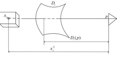
[image:6.595.200.427.86.198.2]

x

Figure 4. Position constraint.

The input for our patches generation approach is multiple depth images and their associated confidence maps, denoted asD1,...,DNandC1,...,CN, respectively. First, the 3D space is discretized as voxels and for every

voxel we need to determine whether there is a surface patch attached to it. Consequently, we consider patches whose center and orientation are restricted to regular voxels and all six unit directional vectors pointing to its neighboring voxels. Let us assume that a patchPax e, with its center position

x

and orientation

e

k,k1,...,6. The

patch is examined whether or not it is consistent with the depth images and should be accepted as a validate patch candidate. The patch is projected to every depth imageDiand checked with the following constraints:

(1) Position constraint. While projecting the patch to camera viewi, we have _{( , , )}1 2 3

c c c c

x  x x x and p respectively representing the camera coordinate and the pixel coordinate for the patch’s center position

x

. As shown in Fig. 4, 3

c

x andD pi( )represent the real depth between the principle plane and the position

x

and the estimated depth fromDi, respectively. The position constraint is satisfied if the difference between

the two depth values is sufficiently small 3

(xcD pi( ) )and



is set to be the distance between two neighboring voxels in our experiments.

(2) Visibility constraint. The constraint is exploited using orientation of patchPa_{x e,} and the camera view direction. Let

v

be the viewing direction of camera

i

given by external camera parameters, the patch is visible to cameraiifv ecos( ) , where



is set to be 3in our experiments.

(3) Confidence constraint. The confidence constraint is exploited using depth confidence maps, which can be used to filter unreliable depth. Letpbe the pixel coordinate while the patch center is projected to depth imageDi, the depth gives validate vote to the patch only ifC pi( ) , whereis set to be 0.4 in all

experiments.

Finally, for the current patchPax e, , if there are more than one depth images that satisfy these three conditions, Pax e, is then accepted as a reliable patch and those corresponding color images are registered as supporting images of the patch.

Next, we need to compute the photo-consistency score for the patches. As the above patches with regular center position and only six candidate orientations cannot sufficiently represent the object surface and the photo-consistency computation is inaccurate when back projecting the patch to its supporting color images. As a result, it is necessary to enforce refinement to the patches. As suggested in [17], conjugate gradient method is used to determine optimal patches by maximizing the following NCC score,

, ( )

2

( ', ') | ( ) | (| ( ) | -1) ij

i j S Pa

C C x n

S Pa S Pa 





(7)

where (S Pa)are the supporting images for the initial patchPax e, ,x'andn'are the center position and orientation for the current patch, and Cijrefers to the NCC score when the current patch is back projected to imagesi j,

[image:7.595.173.424.84.215.2]

(a) (b)

Figure 5. Computed patches for sparse temple set: (a) and (b) shows the rendered patches from different viewpoints， and the number of the computed patches is 208303. The patches are not dense enough in the stair areas due to the occlusion problem and limited viewpoints.

The patch refinement method can find delicate patches as described in [17]. However, the optimization approach is quite time-consuming. In this paper, we utilize the confidence maps as guidance to determine the delicate patches in a quite simple way. For a particular patchPax e, , the image which achieves maximum confidence score among its supporting images is selected as the reference image, denoted asDref. The estimated

depth value and surface normal for the corresponding pixel ofPax e, in the reference image are denoted as ( )

ref

D p andNref( )p , respectively. The center position and orientation for the patch are calculated by transforming these two vectors to the global coordinate. Finally, Eq. (4) is used to compute the consistency score for the current patch. Without considering the computation time, we can further exploit iterative refinement to obtain more accurate photo-consistency score with our computed patches as good initials. The patches extracted from the sparse temple dataset are given in Fig. 5.

5. Geodesic Distance for Regional Term

Although geodesic segmentation can robustly segment long, thin structures, the lack of an explicit edge-finding component may cause geodesic segmentation to come close to but bot precisely localize object boundaries. In [27], Brian L. Price proposed to combine geodesic-distance region information with explicit edge information in a graph-cut optimization framework, which achieves much better foreground/background segmentation results. The explicit edge detection term corresponds to the boundary term in 3D reconstruction function, which is constructed using the photo-consistency score. In this paper, an adaptive regional term based on 3D geodesic distance is defined using the above generated patches in Section 4. This regional term is then combined with boundary term satisfying minimization of the weighted surface function in Eq. (1), so that the reconstructed surface can obtain smoothness while preserving protrusions of the object.

First of all, appropriate seeds are needed to compute the geodesic distance for voxels in 3D space, which correspond to the user marks or “scribbles” on parts of the desired foreground and background regions for 2D image segmentation. The seeds inside or outside the object are denoted asFandB, respectively.

{ | }

{ | }

F

B

v bounding box v is definitely inside the object v bounding box v is definitely outside the object   



  

 (8)

In this paper, we give two simple methods for obtaining voxel setFandBfrom multiple color or depth

images: 1) visual hull based method - Volumetric visual hull of the object should be reconstructed using multi-view silhouettes segmented from color images. The voxels outside the visual hull is defined asB, while

the voxels which are left after several erosions are defined asF. In this method, an appropriate visual hull

obtain the voxel setFandBwithThreschosen to be as 8~10 times as the voxel size, which is robust even for

objects with big concavities.

For every voxelv, its geodesic distance from nearest foreground or background voxels is computed by ( ) min ( , )

l

l _s

D v d s v 

 (9)

wherelis the set of seeds with labell{ , }F B .

The geodesic distance from any voxelv0to the otherv1according to the estimated patches is given by

0 1 0 1 , 0 1 1 ,

0 1 ₀ ,

( , ) min ( ( )) ( )

v v

v v

l _L l v v

d v v 



W L p L p dp (10)

whereLv v0,1( )p is a path parameterized byp[0,1]connectingv0tov1respectively, andW Ll( v v0 1, ( ))p represents

the geodesic weight defined by patches computed in Section 4. For one particular voxel which is inside the object, the weight for background distanceW_Bis assigned a high value when passing through the object surface. For one particular voxel which is outside the object,WFis also assigned a high value when passing through the

surface. Since the refined patches are supposed to give a good approximation of the surface, the geodesic weight is defined by Eq. (11) and Eq. (12), wherev'andv''are two neighboring voxels linked by pathLv'v''andnis the orientation of the patch passed by. The patches covering the surface are assumed to have orientations pointing outward the object.

' ''

1 ( '' ') 0

( )

0

B v v

v v n W L otherwise      

 (11)

' ''

1 ( '' ') 0

( )

0

F v v

v v n W L otherwise      

 (12)

As defined in Eq. (10-12), the background and foreground geodesic distance for the voxels inside the object is assigned a positive value and 0, respectively. On the contrary, for voxels outside the object, the above distances should be 0 and a positive number, respectively. The regional term can be defined in the following and the computed value is displayed in Fig. 6(b). The figure gives a clear explanation of the regional term. As you can see, voxels inside the surface near the protrusions are labeled as strong inside value to prevent shorter-cut.

( )v D v_F( ) D v_B( )

  

(13)

[image:8.595.106.503.500.634.2]

(a) (b) (c)

Next, we weight the adaptive regional term and the boundary term based on the local confidence of the geodesic components using Eq. (14). The spatially varying weighting is introduced to decreases the potential for shortcutting in object interiors while transferring greater control to the boundary term for better localization near object surface. To be more specific, the value of D vF( ) and D vB( ) for voxels near the surface tend to be

similar and therefore the boundary term should play a more important role. Finally, we redefine the energy function of Eq. (1) as follows.

( ) ( ) ( )

( ) ( )

F B

F B

D v D v v

D v D v



  



(14)

( ) ( ) ( ) ( )

S V

E S 

_



v dA



v

_



v dV (15) where empirically we have found=2 to 2.5to work well.

The approach proposed in [28] is often used for 2D geodesic distance computation, while it is still a challenging issue for computing geodesic distance in 3D space. To address this issue, in this paper, we proposed to use a simple searching approach: For a given voxelv, the searching direction is restricted to the six directional lines pointing to its six-neighboring directions, and the pseudo-code for computing its foreground geodesic distance for a given voxelvis given in Algorithm 1.

Input：current voxelv,voxel setFandB, set of patchesP

Output：3D foreground geodesic distanceD v_F( )

F

d : 6*1 vector, with initial value 0 // recording the geodesic distance along six directions '

v =v

for all six directionsdirof v do while(1)

v': current voxel ''

v : next voxel along the direction // the next voxel along the current direction

dir

if patch ( , )x n exists betweenv'v''&& ( ''v v n') 0 then // weight(Eq. (12)) d dirF( )d dirF( ) 1

end if

if v''_F || v''is on the boundary of bounding box then break

end if

'v v'' // update the current voxel end while

end for

( ) min ( )

F F

D v  d v // Eq. (9)

Algorithm 1. 3D geodesic distance computation

6. Graph construction

First, the 3D space is decomposed into voxels which correspond to the graph nodes. In this paper, those nodes are connected with a regular 6-neighbourhood grid and those links are called n-links in the graph. Letvi

0

0 ( )

( ),

( )/ | ( ) |,

i j ij

p N v

C if corresponding patch exists between v v w _{C p N v otherwise}



    





(16)

2 2

( ) 1 exp( tan( ( 1)) / ) 4

C  C

      (17)

whereCis an average photo-consistency cost in Eq. (4) of the corresponding patch andis a transfer function that maps the NCC score to a non-negative interval [0,1];v₀denotes the linking center andN v( )₀ is the neighboring points; and



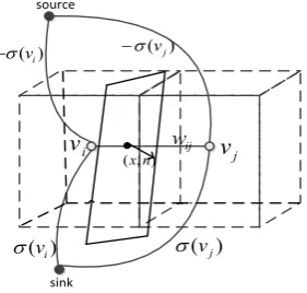
is the fidelity parameter and set to be 0.05 in our experiments. Fig. 6(c) shows the computed patches for one slice.

source

sink

i

v wij

_v

_j

( )vi

 ( )v_j

( )vi



 ( )vj

[image:10.595.230.371.229.363.2]

( , )x n

Figure 7. Graph construction.

In addition, in the constructed graph model each node has a link with the source node and the sink node which represent the probability of being inside or outside the object. The weight is assigned using regional term defined in Section 5. Table 1 gives a clear illumination for the weight assigned to these two kinds of links.

Finally, the minimum cut cost for the above weighted graph corresponds to the minimal energy of the energy function in Eq. (15). The s/t cut separates graph nodes into source or sink set. Letviandvjdenote two

neighboring voxels, whilevibelongs to source set andvjbelongs to sink set. Thenvirefers to a point lying on the

[image:10.595.147.450.550.699.2]

object surface. In other words, the estimated surface is located by inconsistent labeling of neighboring voxels. Using the Poisson Surface Reconstruction method in [15], the 3D points estimated above can be further refined to generate a triangular mesh model and give a good approximation of the object surface as demonstrated in the next section. The octree depth of the PSR used in our experiment is 8 or 10 which are accurate enough.

Table 1. Weight assignment for all links of the graph

link Weights for

{ , }v v_{i j} w_ij { , }v v_{0 1} N

{ , }v s



 v V v ,  B F

 vF

0 vB

{ , }v t



v V v ,  B F

0 v_F

7. Experiments and results

In this section, experimental results on the well-known data set from the multi-view stereo evaluation [29] and also real-world data sets captured from four Kinect cameras are reported. Both visual and quantitative analysis are used to verify the efficacy of the proposed approach as detailed below.

7.1 Evaluation on benchmark data sets

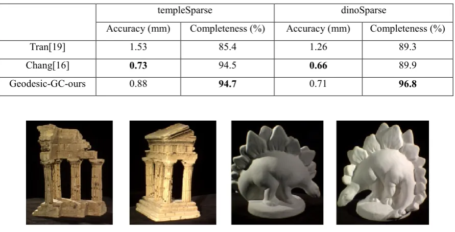
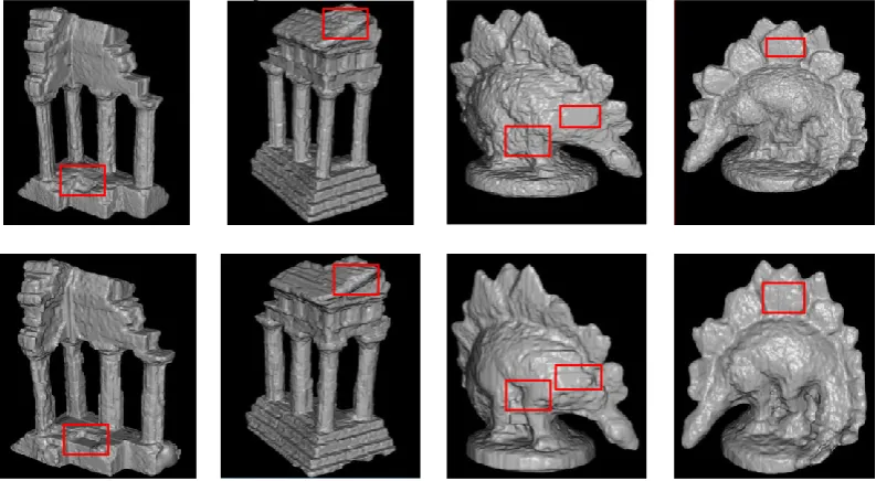
We apply our reconstruction approach on two sparse data sets, templeSparse and dinoSparse, which consists of 16 images respectively, and results of reconstructed mesh models are shown in Fig. 8. As can be seen, our proposed method can generate very satisfying results for both the templeSparse and the dinoSparse data sets. In comparison to the approach proposed in [16], as highlighted in red boxes on the corresponding images in Fig. 8, the additional constraint using the adaptive regional term has greatly improved the results in generating smoother surface while preserving the protrusions.

The proposed method is also quantitatively evaluated on the benchmark data sets, and the evaluation results in terms of accuracy and completeness are given in Table 2 and we make a comparison with another two relevant methods. The compared methods are all based on Graph-cut optimization and Chang[16] and our method achieve relatively high accuracy since we all adopt the patches-based representation. Our method has obvious superior result in completeness.

[image:11.595.76.522.407.634.2]

To be more specifically, the accuracy metric denotes how close the reconstructed surface is to the ground truth model and the completeness metric denotes how much of the object is modeled by our reconstructed surface. The accuracy threshold 90% and completeness threshold 1.25mm are used for all evaluations, which means ninety percent of the reconstructed surface points are near the ground truth with most 0.88mm distance; and the number of the points with 1.25mm to the ground truth is up to 96.8% (for our method). The proposed method shows middle performance for the accuracy comparison and middle-high for completeness comparison. More comparison details are available on the website [29].

Table 2. Quantitative results of our model.

templeSparse dinoSparse

Accuracy (mm) Completeness (%) Accuracy (mm) Completeness (%)

Tran[19] 1.53 85.4 1.26 89.3

Chang[16] 0.73 94.5 0.66 89.9

Figure 8. Reconstruction results on benchmark data sets. The first row displays the color images used in our reconstruction approach. The second row gives the results obtained with original graph cuts method using surfel representation [16]. The third row gives the models reconstructed using our proposed approach. Red boxes are used to highlight the differences between the two group of results.

7.2 Evaluation on real-world data sets

[image:12.595.100.497.85.303.2]

Our approach is further evaluated on depth images captured using multiple Kinects. As it is non-trivial issue for obtaining camera parameters of the depth sensor, the depth image is directly mapped into color sensor view. Fig. 9 shows the color images captured using four Kinects and their corresponding depth images after denoising. The RGB cameras are calibrated using Zhang’s method and further registration [30] are applied to these depth images. The depth images are quite sparse compared with the data used in KinectFusion [31].

Figure 9. Images captured using four Kinects.

[image:12.595.91.525.466.622.2]

in Fig. 10(d).

(a) (b) (c) (d)

Figure 10. Reconstructed model using different methods: (a) is the result generated using state-of-art range images integration [4], (b) is the result using graph-cut [1], (c) gives the reconstructed model from graph-cut yet with our proposed adaptive regional term, respectively; (d) is the rendered results of (c).

8. Conclusion

In this paper, an adaptive 3D geodesic-distance based regional term is proposed and combined into the graph-cut framework to solve the shorter-cuts problem. The patch-based representation is exploited to achieve more accurate photo-consistency computation for the boundary term in the energy function and the computed patches are used to define the 3D geodesic distance for each voxel. Finally, these two terms are combined into the graph-cut framework and the surface is extracted using graph-cut based energy minimization. The experimental results on both well-known datasets and real-world datasets have shown the validity of our proposed approach.

Acknowledgements

This paper is supported by the National High Technology Research and Development Program ("863"Program) of China (No. 2012AA011803).

References

[1] Vogiatzis G, Torr P H S and Cipolla R (2005) Multi-view stereo via volumetric graph-cuts. In Proc. IEEE Conf. Computer Vision and Pattern Recognition (CVPR), San Diego, June 2005, 391-398.

[2] Vu H H, Labatut P, Pons J P and Keriven R. (2010) High accuracy and visibility-consistent dense multi-view stereo.

IEEE Trans. Pattern Analysis and Machine Intelligence, 34(5), 889-901.http://dx.doi.org/10.1109/TPAMI.2011.172 [3] Campbell N D F, Vogiatzis G, Hernández C and Roberto Cipolla (2008) Using multiple hypotheses to improve

depth-maps for multi-view stereo. In Proc. 10th _{European Conf. Computer Vision (ECCV), Oct. 2008, 766-779.} [4] Curless B and Levoy M (1996) A volumetric method for building complex models from range images. In Proc. the

23rd Annual Conf. Computer Graphics and Interactive Techniques,New Orleans, Aug. 1996, 303-312.

[5] G. Turk and M. Levoy. Zippered polygon meshes from range images. In Proc. of SIGGRAPH ’94, Orlando, July 1994, 311–318.http://dx.doi.org/10.1145/192161.192241

[6] Zach C, Pock T and Bischof H (2007) A globally optimal algorithm for robust TV-L range image integration. In Proc.

IEEE Int. Conf. Computer Vision (ICCV), Rio de Janeiro, Oct. 2007, 1-8.

[7] Garcia-Dorado I, Demir I and Aliaga D G (2013). Automatic urban modeling using volumetric reconstruction with surface graph cuts. Computers & Graphics, 37(7), 896-910. http://dx.doi.org/10.1016/j.cag.2013.07.003

[8] Guillemaut J Y and Hilton A (2011) Joint multi-layer segmentation and reconstruction for free-viewpoint video applications. Int. Journal of Computer Vision, 93(1), 73-100. http://dx.doi.org/10.1007/s11263-010-0413-z

[9] Campbell N D F, Vogiatzis G, Hernandez C and R. Cipolla (2010) Automatic 3D object segmentation in multiple views using volumetric graph-cuts. Image and Vision Computing, 28(1), 14-25.

[image:13.595.96.525.109.225.2]

[10] Kolev K, Pock T, Cremers D (2010) Anisotropic minimal surfaces integrating photoconsistency and normal information for multiview stereo, In Proc. 11th _{European Conf. Computer Vision, Greece, Sept. 2010, 538-551.} [11] Schroers C, Zimmer H, Valgaerts L,Bruhn A, Demetz O and Weickert J (2012) Anisotropic range image integration.

Pattern Recognition, 7476, 73-82. http://dx.doi.org/10.1109/TVCG.2009.88

[12] Liu Y, Dai Q and Xu W(2010). A point-cloud-based multiview stereo algorithm for free-viewpoint video. IEEE Trans. Visualization and Computer Graphics, 16(3), 407-418.

[13] Song P, Wu X and Michael W (2010) Volumetric stereo and silhouette fusion for image-based modeling. Int.Journal of Computer Graphics, 26(12), 1435-1450.

[14] Li J, Li E, Chen Y, Lin X and Zhang Y (2010) Bundled depth-map merging for multi-view stereo.In Proc. IEEE Conf. on Computer Vision and Pattern Recognition (CVPR), San Francisco, June 2010, 2769-2776.

[15] Kazhdan M, Bolitho M, Hoppe H (2006) Poisson surface reconstruction. In Proc. 4th _{Eurographics Symposium on}

Geometry Processing, Cagliari, June 2006, 61-70.

[16] Chang J Y, Park H, Park I K, et al. (2011) GPU-friendly multi-view stereo reconstruction using surfel representation and graph cuts. Computer Vision and Image Understanding, 115(5), 620-634.

http://dx.doi.org/10.1016/j.cviu.2010.11.017

[17] Furukawa Y and Ponce J (2010) Accurate, dense, and robust multiview stereopsis. IEEE Trans. Pattern Analysis and Machine Intelligence, 32(8), 1362-1376. http://dx.doi.org/10.1109/TPAMI.2009.161

[18] Wan M, Wang Y, Bae E, Tan X and Wang D (2013) Reconstructing open surfaces via graph-cuts. IEEE Trans. Visualization and Computer Graphics, 19(2), 306-318. http://dx.doi.org/10.1109/TVCG.2012.119

[19] Tran S, Davis L (2006) 3D surface reconstruction using graph cuts with surface constraints. In Proc. 9th European Conf. on Computer Vision, Graz, May 2006, 219-231.

[20] Hernández C, Vogiatzis G and Cipolla R (2007) Probabilistic visibility for multi-view stereo. In Proc. IEEE Conf. Computer Vision and Pattern Recognition (CVPR), Minneapolis, June 2007, 1-8.

[21] Ladikos A, Benhimane S, Navab N (2008) Multi-View Reconstruction using Narrow-Band Graph-Cuts and Surface Normal Optimization. In Proc. British Machine Vision Conf., Leeds, Sept. 2008, 1-10.

[22] Bai X and Sapiro G (2009) Geodesic matting: A framework for fast interactive image and video segmentation and matting. Int. Journal of Computer Vision, 82(2), 113-132. http://dx.doi.org/10.1007/s11263-008-0191-z

[23] Heo Y S, Lee K M, Lee S U (2011) Robust stereo matching using adaptive normalized cross-correlation. IEEE Transactions on Pattern Analysis and Machine Intelligence, 33(4), 807-822.

http://dx.doi.org/10.1109/TPAMI.2010.136

[24] Matyunin S, Vatolin D, Berdnikov Y and Smirnov, M (2011) Temporal filtering for depth maps generated by kinect depth camera. In Proc. 3DTV Conf., Antalya, May 2011, 1-4.

[25] Zuo X and Zheng J (2013) A Refined Weighted Mode Filtering Approach for Depth Video Enhancement. In Proc. Int. Conf. Virtual Reality and Visualization, Xi’an, Sept., 138-144.

[26] McIlhagga W (2011) The Canny edge detector revisited. Int. Journal of Computer Vision, 91(3), 251-261. http://dx.doi.org/10.1007/s11263-010-0392-0

[27] Price B L, Morse B, Cohen S (2010) Geodesic graph cut for interactive image segmentation. In Proc. IEEE Conf. Computer Vision and Pattern Recognition (CVPR), San Francisco, June 2010, 3161-3168.

[28] L. Yatziv, A. Bartesaghi and G. Sapiro (2006) On implementation of the fast marching algorithm. Journal of Computational Physics, 212, 393–399. http://dx.doi.org/10.1016/j.jcp.2005.08.005

[29] http://vision.middlebury.edu/mview/eval/

[30] Toldo R, Beinat A and Crosilla F (2010) Global registration of multiple point clouds embedding the Generalized Procrustes Analysis into an ICP framework.3DPVT 2010 Conf. Paris, France, May 2010, 1-7.