Peridynamics for anti-plane shear and torsional deformations

1

Peridynamics for anti-plane shear and torsional deformations

Selda Oterkus, Erdogan Madenci*

Department of Aerospace and Mechanical Engineering, The University of Arizona, Tucson, AZ 85721, USA

Abstract

A rod or beam is one of the most widely used members in engineering construction. Such members

must be properly designed to resist the applied loads. When subjected to anti-plane (longitudinal) shear

and torsional loading, homogeneous, isotropic, and elastic materials are governed by the Laplace equation

in two dimensions under the assumptions of classical continuum mechanics, and are considerably easier

to solve than their three-dimensional counterparts. However, when using the finite element method in

conjunction with linear elastic fracture mechanics, crack initiation and its growth still pose computational

challenges, even under such simple loading conditions. This difficulty is mainly due to the mathematical

structure of its governing equations, which are based on the local classical continuum theory. However,

the nonlocal peridynamic theory is free of these challenges because its governing equations do not contain

any spatial derivatives of the displacement components, and thus, are valid everywhere in the material.

This study presents the peridynamic equation of motion for anti-plane shear and torsional deformations,

as well as the peridynamic material parameters. After establishing the validity of this equation, solutions

for specific components that are weakened by deep edge cracks and internal cracks are presented.

Keywords: Peridynamics, nonlocal, anti-plane shear, torsion, fracture

*_{Corresponding author. Tel.: +1 520 621 6113.}

2

Prediction of structural failure loads due to crack initiation and propagation is still a challenging area

of solid mechanics. Many different techniques are proposed and widely used within the scope of classical

continuum mechanics. The traditional approaches to predict failure usually employ concepts from linear

elastic fracture mechanics (LEFM). The major drawback of LEFM is the requirement of a pre-existing

initial crack in the structure. Hence, it is not capable of predicting crack initiation. Furthermore, the

mathematical formulation results in unphysical (singular) stress values at the crack tips. To overcome

these problems, cohesive zone models (CZM) and extended finite element methods (XFEM) are widely

accepted as an alternative and implemented in the commercially available finite element analysis

programs.

Although relatively new, peridynamics (PD), introduced by Silling [1] by reformulating the classical

continuum mechanics equations, is very suitable for failure analysis of structures because it allows cracks

to grow naturally without resorting to external crack growth laws. PD is based on integro-differential

equations as opposed to the partial differential equations of classical continuum mechanics. An extensive

literature survey on peridynamics is given by Madenci and Oterkus [2]. A comparison study between

peridynamics, CZM, and XFEM techniques by Agwai et al. [3] highlights the capability of the PD theory.

They showed that the crack speeds obtained from all three approaches are of the same order; however, the

fracture paths obtained through the PD theory are much closer to the experimental results than those of

the other two techniques.

The numerical simulation of three-dimensional structures can be computationally costly. Although all

structures are three dimensional in nature, they can be idealized under certain assumptions. Under such

idealization, a rod or a beam subjected to anti-plane (longitudinal) shear and torsional loading can be

analyzed in two dimensions. However, the PD equation of motion and the PD material parameter must

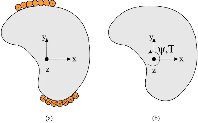
reflect these idealizations. As shown in Figure 1, this study presents the derivation of the PD equation of

3

establishing its validity by comparing against benchmark solutions, a study of components that are

weakened by deep edge cracks and internal cracks is presented.

(a) (b)

Figure 1. A beam under (a) anti-plane shear and (b) torsion.

2. Kinematics for anti-plane shear and torsional deformation

Due to the nature of loading and the geometry of the components, the deformation of the cross section

on the -z plane is dependent only on the -x and -y coordinates. Also, the cross section of the component remains uniform. At any instant of time, every point in the material denotes the location of a material

particle, and these infinitely many material points (particles) constitute the continuum. In the undeformed

state of the body, each material point is identified by its coordinates, x_{( )k} with (k1,2,..., ) , and is

associated with an incremental volume, V_{( )k} , and a mass density of (x_{( )k} ). Each material point can be subjected to prescribed body loads, displacement, or velocity, resulting in motion and deformation.

According to the PD theory introduced by Silling [1], the motion of a body is analyzed by considering

the interaction of a material point, x_{( )k} , with the other, possibly infinitely many, material points, x_{( )j},

4

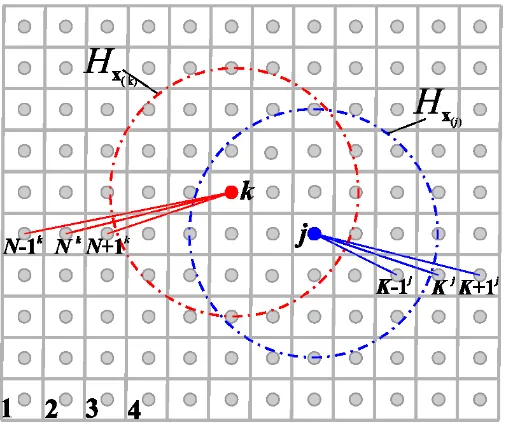
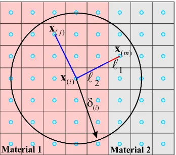
interacting with x_{( )k} is assumed to vanish beyond a local region (horizon), denoted by H_{x( )k} , shown in Figure 2. Similarly, the material point x_{( )j} interacts with the other material points in its own family,

( )j

Hx

. The range of the material point x_{( )k} is defined by , _{referred to as the “horizon.” Also, the material} points within a distance  of x_{( )k} are called the family of x_{( )k} ,

( )k

H_x . The interaction of material points is prescribed through the micropotentials that depend on the deformation and constitutive properties of the

material.

As shown in Figure 2, material point x_{( )k} interacts with its family of material points,

( )k ,

H_x and is

influenced by the collective deformation of all these material points. Similarly, the material point x_{( )j} is

influenced by deformation of the material points,

( )j,

H_x in its own family.

5

With respect to a Cartesian coordinate system, the material point ( ) { ( ), ( ), ( )}

T

k  xk yk zk

x experiences

displacement, ( ) { ( ), ( ), ( )}

T

k  uk vk wk

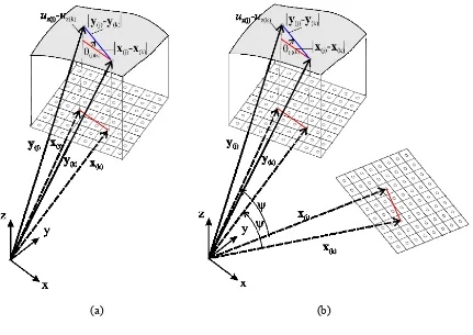
u , and its location is described by the position vector y_{( )k} x_{( )k} u_{( )k} in

the deformed state, as shown in Figure 3. The body load vector at material point x_{( )k} is represented by

( ) {0,0, ( )}

T

k  bz k

b , respectively. The motion of a material point conforms to the Lagrangian description. In

the deformed configuration, the material points x_{( )k} and x_{( )j} experience displacements u_{( )k} and u_{( )j} ,

respectively. Their initial relative position vector (x_{( )j} x_{( )k} ) prior to deformation becomes (y_{( )j} y_{( )k} )

after deformation.

Under anti-plane and torsional loadings, the initial position of material points x_{( )j} and x_{( )k} for

( )j ( )k

z z z can be defined as _{( )}T { _{( )}, _{( )}, } j  xj yj z

x and _{( )}T { _{( )}, _{( )}, }

k  xk yk z

x . Their initial relative position

can then be expressed as

( ) ( ) ( ) ( ) ( ) ( )

( T T ) {( ),( ),0}

j  k  x j xk yj yk

x x (1)

For anti-plane shear deformation, these material points experience the displacements:

( ) {0,0, ( )} and ( ) {0,0, ( )}

T T

j  uz j k  uz k

u u . Their relative position in the deformed state becomes





( )j  ( )k  ( )j  ( )k  uz j( )uz k( ) z

y y x x e (2)

For torsional deformation, these material points experience the displacements:

( ) { ( ), ( ), ( )}

T

j  zyj zx j uz j

u and _{( )}T { _{( )}, _{( )}, _{( )}}

k  zyk zxk uz k

u , in which  represents the angle of twist.

Their relative position can be expressed as





( )j  ( )k  ( )j  ( )k  ( ( )j  ( )k ) uz j( )uz k( ) z

y y x x x x e (3)

in which _{ }T {0,0,_z}_{, and the product term}

( ) ( )

( _{j k} )

 x x represents the rotation of (x_{( )j} x_{( )k} )

6

As shown in Figure 3, the relative out-of-plane displacement (elevation) of material points x_{( )j} and x_{( )k}

is defined as

( )( )k j z j( ) z k( )

e u u (4)

Also, the slope of this elevation (change in angle) between material points x_{( )k} and x_{( )j} is defined as

( )( ) ( ) ( ) ( )( )

( )( ) ( )( )

k j z j z k

k j

k j k j

e u u

r

 



  (5)

where _{( )( )k j} |x_{( )j} x_{( )k} | represents the distance between these material points.

(a) (b)

7

Due to the interaction between material points x_{( )k} and x_{( )j} , a scalar-valued micropotential, w_{  k j} , develops; it depends on the material properties, as well as the elevation, e_{( )( )k j} , between point x_{( )k} and all other material points in its family. Note that w_{  j k} w_{  k j} because w_{  j k} depends on the state of material points within the family of material point x_{( )j} . These micropotentials can be expressed as





( )( )k j  ( )( )k j e_{(1 )( )}k _k ,e_{(2 )( )}k _k ,

w w (6a)

and





( )( )j k  ( )( )j k e_{(1 )( )}j _j,e_{(2 )( )}j _j ,

w w (6b)

in which e_{( )( )j k} u_{z j( )}u_{z k( )} represents elevation between material points x_{( )k} and x_{( )j} . The change in elevation, e_(mk_{)( )k} , is measured between point x_{( )k} and the m-th material point that interacts with point

( )k

x . Similarly, e_(mj_{)( )j} is measured between point x_{( )j} and the m-th material point that interacts with point

( )j

x , as shown in Figure 2. The strain energy density, W_{( )k} , of material point x_{( )k} can be expressed as a summation of all the micropotentials, w_{( )( )k j} , arising from the interaction of material point x_{( )k} and the other material points, x_{( )j} , within its horizon in the form









( ) ( )( ) _{(1 )( ) (2 )( )} ( )( ) _{(1 )( ) (2 )( )} ( ) 1

1 1

, , , ,

2 2 k k j j

k k j _{k k} j k _{j j} j

j

W  e e e e V



 





in which w_{( )( )k j} 0 for k j.

The PD equation of motion at material point x_{( )k} can be derived by applying the principle of virtual

work, i.e.

1 0

( ) 0

t

t T U dt





8

( ) ( )

0

z k z k

d L L

dt u u



  

 

 _  _

  (9)

where the Lagrangian L is defined as L T U  .

The total kinetic and potential energies in the body can be obtained by summation of kinetic and

potential energies of all material points, respectively,

( ) ( ) ( ) ( ) 1

1

2 i z i z i i

i

T   u u V







and





( ) ( ) ( ) ( ) ( )

1 1

i i z i z i i

i i

U W V  b u V

 







Substituting for the strain energy density, W_{( )i} , of material point x_{( )i} from Eq. (7), the potential energy can be rewritten as













( )( ) (1 )( ) (2 )( ) ( )( ) (1 )( ) (2 )( ) ( ) ( ) ( ) ( )

1 1

1 1

, , , ,

2 2 _{i j} i _i i _{i j i} j _j j _{j j z i z i i}

i j

U   e e e e V b u V

 

 _{ } 

 _{ }  _  _

 

 

The Lagrangian can be written in an expanded form by showing only the terms associated with the

material point x_{( )k} as

















( ) ( ) ( ) ( )

( )( ) (1 )( ) (2 )( ) ( )( ) (1 )( ) (2 )( ) ( ) ( ) 1

( )( ) (1 )( ) (2 )( ) ( )( ) (1 )( ) (2 )( ) ( ) ( ) 1 1 ... 2 1 1 , , , , 2 2 1 1 , , , , 2 2

k k j j

i i k k

k z k z k k

k j k k j k j j j k

j

i k i i k i k k i k

i

L u u V

e e e e V V

e e e e V V

           _  _        _  _   



w w





... b u_{z k z k} V_k 





(12a)

9





















( )( ) _{(1 )( ) (2 )( )} ( ) ( ) 1

( )( ) (1 )( ) (2 )( ) ( ) ( ) 1 ( ) ( ) ( ) 1 2 1 , , 2 1 , , 2 . k k j j

k z k z k k

k j _{k k} j k

j

j k j j j k

j

z k z k k

L u u V

e e V V

e e V V

b u V

          





Substituting from Eq. (12b) into Eq. (9) results in the Euler-Lagrange equation of the material point x_{( )k}

as

















1 1 ( ) ( ) ( )

( ) ( ) ( )( )

( ) ( ) ( )

1 1 ( ) ( ) ( )

1 2

1

0

2

z j z k k j

k z k k i

j i z j z k z k

z k z j j k

i z k k

j i z k z j z k

u u

u V V

u

u u

u u

V b V

u u u                   _{ }  _   _             _{ }         

 

 









1 1 _{( ) ( )}

( )( )

( ) ( )

1 1 _{( ) ( )}

1 2 1 0 2 k j

k z k i

j i _{z j z k}

j k

i z k

j i _{z k z j}

u V u u V b u u           _            _        _{ }   

 

 

in which it is assumed that the interactions not involving material point x_{( )k} do not have any effect on

material point x_{( )k} . Based on the dimensional analysis of this equation, it is apparent that the quantity

1 ( ) ( )( )/ ( ( ) ( ))

i Vi k i uz j uz k

 

 w   represents the force density in the -z direction that material point x_{( )j}

exerts on material point x_{( )k} and i_{1 ( )}Vi _{( )( )}i k / (uz k_{( )} uz j_{( )})

 

 w   represents the force density in the -z

direction that material point x_{( )k} exerts on material point, x_{( )j} . With this interpretation, Eq. (13b) can be rewritten as





_

_

z k j j k j k i

i

j z j z k

t e t V

V u u

      



x x w (14a)

10





_

_

( )( ) ( )( ) ( ) ( ) ( )

1

( ) ( ) ( )

1 1

, ,

2

i k

z j k k j k j i

i

j z k z j

t e t V

V u u







 _

 

  _{ }

 





x x w (14b)

in which V_{( )j} represents the volume of material point x_{( )j} . The material point x_{( )j} exerts the force density t_{z k j( )( )} on material pointx_{( )k} .

By utilizing the state concept described by Silling et al. [4] and Silling and Lehoucq [5], the force

densities t_{z k j( )( )} and t_{z j k( )( )} can be stored in force scalar states that belong to material points x_{( )k} and

( )j,

x respectively, as









z k z k j z j z j k

t t t t t t

   

   

_{ } _{ }

   

   

x x (15)

The force densities t_{z k j( )( )} and t_{z j k( )( )} stored in scalar states t_z(x_{( )k} , )t and t_z(x_{( )j}, )t can be extracted again by operating the force states on the corresponding initial relative position vectors, (x_{( )j} x_{( )k} ) and

( ) ( )

(x_k x _j ), as









( )( ) z ( ), ( ) ( ) and ( )( ) z ( ), ( ) ( )

z k j k j k z j k j k j

t t x t x x t t x t x x (16)

By using Eqs. (14a) and (14b), the Euler-Lagrange equation of the material point x_{( )k} can be recast as









( ) ( ) ( )( ) ( )( ) ( ) ( ) ( )( ) ( )( ) ( ) ( ) ( ) ( ) 1

, , , ,

k z k z k j j k j k z j k k j k j j z k

j

u t e t t e t V b

 



 





Because the area of each material point V_{( )j} is infinitesimally small, for the limiting case of V_{( )j} 0, the infinite summation can be expressed as a Riemann integral while considering only the material points

within the horizon. Therefore, Eq. (17) can be rewritten in integral equation form as



 



z _H z z z z z z z

u t u u t t u u t dV b

 



11

The force densities at material points x_{( )k} and x_{( )j} can be defined in the form





( )( ) ( )( ) ( ) ( ) ( )( )

1

, ,

2

z k j j k j k k j

t e x x t  A (19a)

and





( )( ) ( )( ) ( ) ( ) ( )( )

1

, ,

2

z j k k j k j k j

t e x x t   B (19b)

where A_{( )( )k j} and B_{( )( )k j} are auxiliary parameters that are dependent on engineering material constants, the deformation field, and the horizon.

In light of the definition (14) of the expressions for force density in terms of micropotentials, the

force density vectors can be related to the strain energy density function , W_{( )k} , at material point x_{( )k} as





_

_

( )( ) ( ) ( ) ( ) ( )

( ) ( ) ( )

1

, , k

z k j z j z k j k

j z j z k

W

t u u t

V u u



  

 

x x (20a)

and





_

_

( )( ) ( ) ( ) ( ) ( )

( ) ( ) ( )

1

, , j

z j k z k z j k j

k z k z j

W

t u u t

V u u



  

 

x x (20b)

However, the determination of the auxiliary parameters, A_{( )( )k j} and B_{( )( )k j} , requires an explicit form of the strain energy density function.

3.2. Peridynamic material parameters

For an isotropic and elastic material experiencing anti-plane and torsional deformation, the classical

expression for the strain energy density, W_{( )k} , at material point x_{( )k} can be written as

2 2

( ) ( ) ( )

1 2

k k xz k yz

12

in which  is the shear modulus of the material, and _{( )k xz} and _{( )k yz} are the transverse shear strain components at material point x_{( )k} .

Analogous to Eq. (21), the PD representation of the strain energy density, W_{( )k} , at material point x_{( )k}

can be expressed as

2 2

( )k ( )k xz ( )k yz

W a r_ r _ (22)

in which a is the ordinary state-based PD material parameter for strain energy and r_{( )k xz} and r_{( )k yz} are defined in the form

( ) ( )( ) ( )( ) ( )( ) ( ) 1

cos N

k xz k j j k k j j

j

r b w e  V







and

( ) ( )( ) ( )( ) ( )( ) ( ) 1

sin N

k yz k j j k k j j

j

r b w e  V







in which cos_{( )( )k j} (x_{( )j} x_{( )k} ) /_{( )( )k j} and sin_{( )( )k j} (y_{( )j} y_{( )k} ) /_{( )( )k j} , N represents the number of material points within the family of x_{( )k} , and b is an unknown PD parameter. The non-dimensional

influence function, which can be taken in the form of w_{( )( )k j}  / _{( )( )k j} , provides a means to control the influence of material points away from the current material point at x_{( )k} . The infinitesimal volume of the

material point, x_{( )j} , is denoted by V( )j  ( )( )k j( )( )k j( )( )k j , where ( )( )k j and ( )( )k j represent the incremental distance and angle between material points x_{( )k} and x_{( )j} and is the length of the component.

As the horizon approaches zero, the out-of-plane displacement at material point x_{( )j} can be expressed by using a Taylor series expansion as

2 2

( ) ( ) ( ( )( ) ( )( ) ( )( ) ( )( ) ( )( ) ( )( )

2 2 2

( )( ) ( )( )

), ( ), ( ),

( ), ( )( ) ( ), ( )( ) ( )( )

cos sin cos

1 2 1

2

cos sin sin

z j z k z k j k j z k j k j z k j k j

z k j k

k x k y k xx

k xy j k j zk yy k j k j

u u u u u

u u

     

    

   

 

13

Substituting from Eq. (24) into Eq. (23) along with the infinitesimal volume and influence function,

performing algebraic manipulations, and converting the summations to integrations lead to

3

( ) ( ),

2

k xz z k x

r b  u (25a)

and

3

( ) ( ),

2

k yz z k y

r b  u (25b)

Defining _{b2 / ( }3_{) reduces} ( )k xz

r and r_{( )k yz} to the classical transverse shear strains _{( )k xz} and _{( )k yz}; thus, equating the peridynamic and classical strain energy density, W_{( )k} , at material point x_{( )k} results in

2 2 2 2

( ) ( ) ( ) ( ) ( )

1 2

k k xz k yz k xz k yz

W a r_ r _  _  _ (26)

It yields the ordinary state-based peridynamic material parameter for strain energy as

1 2

a  (27)

which is not dependent on the horizon, unlike the parameter b.

3.3. Force density-displacement relation

Substituting for W_{( )k} in Eq. (20) and differentiating, the force density, t_{z k j( )( )}, can be obtained as





( )( ) ( ) ( ) ( ) ( ) ( )( ) ( ) ( )( ) ( )

( )( ) ( )( )

, , j k j k

z k j z j z k j k k j k xz k j k yz

k j k j

x x y y

t u u t  w r w r

 

   

   _  _

 

 

x x (28a)

_{( )( )}





( )( ) ( )( )

, , k j k j

z j k z k z j k j j k j xz j k j yz

k j k j

x x y y

t u u t  w r w r

 

   

   _  _

 

 

x x (28b)

Comparison of Eqs. (28) and (19) leads to the determination of A_{( )( )k j} and B_{( )( )k j} as

( ) ( ) ( ) ( )

( )( ) ( )( ) ( ) ( )( ) ( )

( )( ) ( )( )

2 j k j k

k j k j k xz k j k yz

k j k j

x x y y

A  w r w r

 

   

   

 

14

( ) ( ) ( ) ( )

( )( ) ( )( ) 2 ( ) ( )( ) 2 ( )

( )( ) ( )( )

2 j k j k

j k j k j xz j k j yz

k j k j

x x y y

B  w r w r

 

   

   

 

  (29b)

After substituting for the force densities, the final form of the equation of motion becomes









( ) ( ) ( )( ) ( ) ( ) ( ) ( ) ( ) ( )

1 ( )( ) ( )( )

j k j k

k z k k j k xz j xz k yz j yz j z k

j k j k j

x x y y

u w r r r r V b

           _    _     



( ) 3 ( )( ) ( )( ) ( )( ) ( ) 1

2

cos N

k xz k j j k k j j

j

r w e  V

 





( ) 3 ( )( ) ( )( ) ( )( ) ( ) 1

2

sin N

k yz k j j k k j j

j

r w e  V

 





4. Bond-based peridynamics

In the case of pairwise interaction only between material points x_{( )i} and x_{( )j} , the micropotential,

  i j

w , is a function of e_{( )( )i j} . Thus, the total potential energy can be obtained by the summation of the micropotentials w_{( )( )i j}(e_{( )( )i j} ) arising from deformation only between two material points within the same family













( )( ) ( )( ) ( )( ) ( )( ) ( ) ( ) ( ) ( )

1 1

1 1

2 2 i j i j j i j i j z i z i i

i j

U   e e V b u V

 

 _{ } 

 _{ }  _  _

 

 

For a pairwise interaction, the Euler-Lagrange equation results in

















( ) ( ) ( )( )

( ) ( ) ( )

1 ( ) ( ) ( )

( ) ( ) ( )( )

( ) ( )

1 ( ) ( ) ( )

1 2

1

0

2

z j z k k j

k z k k

j z j z k z k

z k j

j k

z k k

j z k z j z k

u u u V u u u u w b V u u u                  _  _                      





15

k z k z k j z j k j z k

j

u f f V b

 



 





in which f_{z k j( )( )} and f_{z j k( )( )} are defined as









( )( ) ( )( )

( ) ( ) ( ) ( )

and

k j j k

z k j z j k

z j z k z k z j

f f

u u u u

 

 

   

w w

(34a,b)

They represent the PD interaction forces between the material points x_{( )k} and x_{( )j} arising from the

deformation (elevation). For a linear material behavior, they can be defined in the form

( )( ) ( )( ) and ( )( ) ( )( )

z k j k j z j k j k

f cr f cr (35a,b)

or

( )( ) ( )( ) and ( )( ) ( )( )

z k j k j z j k k j

f cr f  cr (36a,b)

With these definitions, the equation of motion, Eq. (33), becomes

( ) ( )( ) ( ) ( ) 1

z k k j j z k

j

u c r V b

 







or

( ) ( )

( ) ( ) ( )

1 ( )( )

z j z k

z k j z k

j k j

u u

u c V b















in which c is the PD material parameter (bond constant) associated with the anti-plane and torsional deformations.

As the horizon approaches zero, Eq. (37) must recover its classical counterpart, given as





z z xx z yy

u u u

   (38)

Representing the out-of-plane displacement at material point x_{( )j} by using a Taylor series expansion as in

Eq. (24), substituting it into Eq. (37) along with the infinitesimal volume, and performing algebraic

manipulations after converting the summations to integrations lead to





3

( ) ( ), ( ),

6

z k z k xx z k yy

u c  u u

16

Comparison of the bond-based PD equation of motion with its classical counterpart leads to the

determination of the PD bond constant, c, as

3

6

c 

 

 (40)

which is dependent on the horizon. The final form of the bond-based PD equation of motion becomes

( ) ( )

( ) 3 ( )

1 ( )( )

6 z j z k

z j j

j k j

u u

u  V



  











Alternatively, in light of Eq. (34) and (35), the bond constant can also be determined by considering the

explicit expression for the micropotentials in the form

2 2

( )( ) ( )( ) ( )( ) ( )( ) ( )( ) ( )( )

1 1

and

2 2

k j  ck jrk j j k  ck jrj k

w w (42a,b)

Therefore, the strain energy density at material point x_{( )k} can be obtained from Eq. (7) as

2 ( ) ( )( ) ( )( ) ( )

1

1 1

2 2

k k j k j j

j

W c   r V







Substituting for the slope and infinitesimal volume and converting the summation to integration lead to





k z j z k

W c u u d d

 

 



_{ }

The peridynamic bond constant, c, can be determined by equating the strain energies from classical continuum mechanics and peridynamics for a specified simple deformation such as ( , ) (w x y  x y ). For the material point of interest located at (x_{( )k} 0,y_{( )k} 0), the elevation is e_{( )( )k j} (xy) and

2 2

( )( )k j x y

      . Thus, the peridynamic strain energy density can be obtained as





2 2 3

2 ₂

( ) ( ) ( )

0 0 0 0

1 1 1 1

2 2 2 2 6

k z j z k

c

W c u u d d c d d

    _

    



_{ }

_{ }

17









, ,

1 1

2 xz xz yz yz 2 z x z y

W        u u  (46)

Equating the strain energies from peridynamics and the classical continuum mechanics leads to the

determination of the PD material parameter, _{c6 /  }3_{, which is the same as in Eq. (40).}

5. Correction of PD material parameters

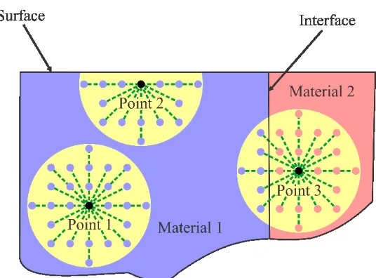
The PD material parameters b and c are determined for material points with a horizon completely embedded in the material. The values of these parameters depend on the domain of integration defined by

the horizon. Therefore, their values require correction if the material point is close to free surfaces or

material interfaces (Figure 4). Since the presence of free surfaces is problem dependent, it is impractical

to resolve this issue analytically.

Figure 4.Surface effects in the domain of interest.

5.1. Surface correction

The bond-based and ordinary state-based PD parameters are corrected by comparing the PD and

18

loading conditions. The correction for the parameter c is achieved by comparing the strain energy densities, and for the parameter, b by comparing the shear strain components.

The first loading case is a simple linear displacement distribution in the x-direction given by

z

u x (47)

The second loading case is a simple linear displacement distribution in the -y direction given by

z

u y (48)

Due to these loading conditions, the corresponding PD strain energy density and shear strain can be

obtained from Eqs. (43) and (23) as





2

( ) ( ) ( ) ( )

1 ( )( )

1 1 1

2 2

N PD

k x j k j

j k j

W  c x x V













( ) ( ) ( ) ( )

1 ( )( )

1 1 1

2 2

N PD

k y j k j

j k j

W  c y y V









and

( ) (

( ) ( )( ) (

1

) ( ) ) ( )

( _{j k} )cos

N

k xz k j k j j

j

x

r b w x  V







1

) ( ) ) ( )

( _{j k} )sin

N

k yz k j k j j

j

y

r b w y  V







with N representing the number of material points inside the horizon of x_{( )k} . For these loading

conditions, the classical strain energy of a material point _{( )}CCM k

W and shear strain components are

2 ( ) 1 2 CCM k x

W   and 2

( )

1 2 CCM k y

W   (51)

and

( )k xz

  and _{( )k yz} (52)

The correction factors for these loading conditions at material point x_{( )k} can be determined as

( ) ( )

( )

CCM k x

x k PD

k x

W g

W

 and ( )

( ) ( ) k xz k xz k xz g r 

 (53)

and ( ) ( ) ( ) CCM k y

y k PD

k y

W g

W

 and ( )

( ) ( ) k yz k yz k yz g r 

19

With these correction factors, the final form of the ordinary state-based PD equation become









( ) ( ) ( )( ) ( ) ( ) ( ) ( ) ( ) ( ) ( ) ( ) ( )

1 ( )( ) ( )( )

( )

j k j k

k z k k j k xz k xz j xz j xz k yz k yz j yz j yz j

j k j k j

z k

x x y y

u w r g r g r g r g V

b            _    _     



k xz k j j k k xz k j j

j

r b w e g  V







1

sin N

k yz k j j k k yz k j j

j

r b w e g  V







For the bond-based parameter, the correction factors can be obtained by taking their mean value as

( ) ( ) ( )( )

2 x k x j k j x

g g

g   and ( ) ( )

( )( )

2 y k y j k j y

g g

g   (57)

which may represent the principal axis of an ellipsoid. The correction factor between arbitrary material

points x_{( )k} and x_{( )j} can be calculated by



 



( )( )k j x ( )( )k j x y ( )( )k j y

G _ n g  n g _

  (58)

where n_x and n_y are direction cosines of n(x_{( )j} x_{( )k} )/ |x_{( )j} x_{( )k} |. The final form of the bond-based PD equation including the correction factor for material point x_{( )k} becomes

( ) ( )

( ) 3 ( )( ) ( )

1 ( )( )

6 z j z k

z k k j j

j k j

u u

u  G V



  











5.2. Dissimilar material interface

The correction at the interface is achieved by using equivalent PD material parameters [6]. As shown

in Figure 5, the material point x_{( )i} may interact with material points x_{( )j} and x_{( )m} . Material points x_{( )i}

20

Because the material points x_{( )i} and x_{( )m} are embedded in two different materials, their material

parameter, a_{  i m} , can be expressed in terms of an equivalent material constant as

   1 2

1 2

1 2

i m

a

a a

 



(60)

in which ₁ represents the segment of the distance between material points x_{( )i} and x_{( )m} in material 1

whose material parameter is a₁, and ₂ represents the segment in material 2 whose material parameter is

2 a .

Figure 5.Interaction of material points across the interface.

6. Boundary conditions

Unlike the local theory, the PD boundary conditions are imposed through a non-zero volume of

fictitious boundary layers. This necessity arises because the PD field equations do not contain any spatial

derivatives; therefore, constraint conditions are, in general, not necessary for the solution of an

integro-differential equation of motion. However, such conditions can be imposed by prescribing constraints on

the displacement or transverse shear stress components in a fictitious boundary layer.

21

This type of boundary condition can be achieved through a fictitious region, R_f . Therefore, a

fictitious boundary layer with depth  _{is introduced along the boundary of the actual material region,} R ,

as shown in Figure 6. Based on numerical experiments, Macek and Silling [7] suggest that the extent of

the fictitious boundary layer be equal to the horizon, , in order to ensure that the imposed prescribed

constraints are accurately reflected in the real domain.

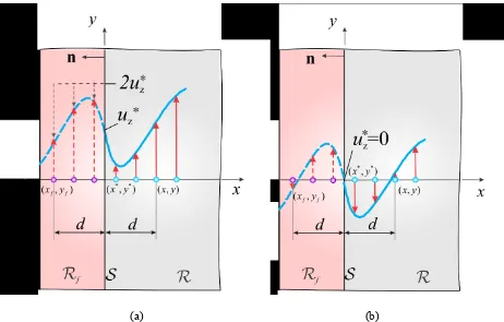
The prescribed boundary value, *_{( , , )}* *

z

u x y t , is imposed through a layer of the fictitious region, R_f , along the boundary of the material surface, S , as

* * *

( , , ) 2 ( , , ) ( , , )

z f f z z

u x y t  t u x y t  t u x y t (61a)

with









 

f f f

x y S x y R x y R (61b)

in which ( , )x y represents the position of a material point in R , and _{( , )x y}* * _{represents the location of a}

point on the boundary surface, S . The location of the image material point in R_{f is denoted by ( ,}x y_{f f}). The implementation of the prescribed boundary value of the displacement is depicted in Figure 6. In the

case of *_{( , , ) 0}* *

z

u x y t  , this condition becomes

( , , ) ( , , )

z f f z

22

(a) (b)

Figure 6 Imposing displacement constraints on the boundary: ( a) non-zero constraint _{( , , )}* * *

z z

u x y t u

and (b) zero constraint _{( , , )}* * * ₀

z z

u x y t u  _.

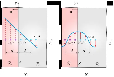
6.2. Conditions on transverse shear stress components

Similar to the displacement boundary conditions, the transverse shear stress conditions are imposed

through a fictitious region, R_f . In the case of anti-plane shear deformation, applied transverse shear

stress on the boundary, _{( , , )}* *

z x y t

 

  with x y, , is imposed as (Figure 7,left)









u

x y t x y

 

  





 

 _{ }



  (63a)

or





u

x y 

 





23

which can be enforced as

1

( , ) ( ) ( , )

z f f f z

u x y  _  u x y



   (63c)

For a zero transverse shear stress condition, i.e., _{( , , ) 0}* *

z x y t



  , this expression reduces to





z z

u x y u x y (64)

In the case of torsional deformation, zero shear stress boundary conditions are imposed as













0

, , z , 0

xz

u

x y t x y y y

x

 _   _ 

  (65a)

and













0

, , z , 0

yz

u

x y t x y x x

y

 _   _ 

  (65b)

or









x y y y

x 

    (66a) and









x y x x

y 

 _{ }

 (66b)

which can be imposed as









1

, ( ) ( , )

z f f f z

u x y  y y x x u x y



    (67a)

and









1

, ( ) ( , )

z f f f z

u x y  x x y y u x y



    (67b)

24

(a) (b)

Figure 7. Material points and their image in the fictitious region for imposing: (a) non-zero flux and (b) zero flux.

7. Failure prediction

Damage is introduced through elimination of interactions (micropotentials) among the material

points. It is assumed that when the change in angle (transverse shear strain), r_{( )( )k j} , between two material points, k and j, exceeds its critical value, r_c, the onset of damage occurs. Damage is reflected in the equations of motion by removing the force density vectors between the material points in an irreversible

manner. Therefore, the force density vectors t_{z k j( )( )} and t_{z j k( )( )} in the case of the ordinary state-based form of the equations of motion and f_{z k j( )( )} and f_{z j k( )( )} in the case of the bond-based form can be modified through a history-dependent scalar-valued function H t x( , _{( )j} -x_{( )k} ) [8] as





( )( ) , ( )- ( ) ( )( )

z k j j k z k j

25





( )( ) , ( )- ( ) ( )( )

z k j j k z k j

f H t x x f and f_{z j k( )( )}H t x









( ) ( )

1 if ( , - ) for all 0

,

-0 otherwise

k j j k c

j k

r t x x r t t

H t x x _{ }    

 (70)

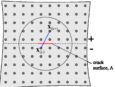
The critical value, r_c, can be determined by equating the amount of energy required to remove all of the micropotentials across a unit crack surface to the critical energy release rate,G_IIIc, for the mode III type of loading of linear elastic fracture mechanics (LEFM). In order to create a new crack surface, A, all of the micropotentials (interactions) between the material points x_(k₎ and x_(j₎ whose line of action

crosses this new surface must be terminated, as sketched in Figure 8. The material points x_(k₎ and x_(j₎

are located above and below the new crack surface, respectively.

Figure 8. Interaction of the material points x_(k₎ and x_(j₎ above and below the crack surface.

Hence, the strain energy required to remove the interaction between two material points x_(k₎and

(j)

26

k j j k

c

k j k j

W       V V 



 w w (71)

Furthermore, the total strain energy required to remove all of the interactions across the newly created

crack surface A can be obtained as

( )( ) ( ) ( ) ( )( ) ( ) ( )

1 1 1 1

1 1 1 1

2 2 2 2

K J K J

c c c

k j k j j k j k

k j k j

W V V V V

   

       

   



 

 

for which the line of interaction defined by _(k_)(j₎|x_(k₎x_(j₎| and the crack surface intersect, and K and J indicate the number of material points above and below the crack surface within the families of

(k)

x and x_(j₎, respectively. If this line of interaction and crack surface intersect at the crack tip, only

half of the critical micropotential is considered in the summation.

Considering only the pairwise interactions between x_(k₎ and x_(j₎ crossing the crack surface, the

micropotentials for linear elastic deformation are given by Eq. (42) as

2 ( )( ) ( )( ) ( )( )

1 2

k j  ck j rk j

w and 2

( )( ) ( )( ) ( )( )

1 2

j k  c j k rj k

w (73)

Their critical values can be expressed as

2 ( )( ) ( )( ) 1 2 cr c k j  ck j r

w and 2

( )( ) ( )( )

1 2 cr

c j k  c j k r

w (74)

Thus, the total strain energy required to remove all of the interactions across the newly created crack

surface A becomes

2 ( )( ) ( ) ( ) 1 1 1 2 K J c

c j k k j

k j

W cr  V V

 

   

 





The amount of energy required to remove all of the interactions (micropotentials) across the unit

crack surface equals the critical strain energy release rate, thus leading to

2 ( )( ) ( ) ( ) 1 1 1 2 K J c

c j k k j

k j IIIc

cr V V

W G A A         

 



27

( )( ) ( ) ( ) 1 1

2 K J

j k k j

k j

V V h A





 

   

  _



(77)

Thus, the critical shear angle can be obtained as

2 3

IIIc c

G

r 



 (78)

The local damage at a point is defined as the weighted ratio of the number of eliminated interactions

to the total number of initial interactions of a material point with its family members [8]









( )

( ) 1

,

-, 1

N

j k j

j

k N

j j

H t x x V

x t

V

 



 





If the local damage value has a value equal to or larger than 0.5, it can be interpreted as the creation of

new crack surfaces.

8. Numerical results

The solution to the PD field equations requires time and spatial integrations while considering

constraints and/or loading conditions, as well as initial conditions. The spatial integration is performed by

using a Gaussian integration (meshless) scheme because of its simplicity, and time integration by using

backward and forward difference explicit integration schemes. The domain is divided into a uniform grid,

with integration or collocation (material) points associated with specific volumes. Associated with a

particular material point, the numerical implementation of spatial integration involves the summation of

the volumes of material points within its horizon. However, the volume of each material point may not be

embedded in the horizon in its entirety, i.e., the material points located near the surface of the horizon

may have truncated volumes. As a result, the volume integration over the horizon may be incorrect if the

entire volume of each material point is included in the numerical implementation. Therefore, a volume

28

The steady-state solution to the PD field equation can be achieved by different techniques; however, in

this study an adaptive dynamic relaxation method (ADR) is employed (described in detail by Madenci

and Oterkus [2]).

The capability of the PD theory is demonstrated by considering (1) a square bar under anti-plane

shear loading, (2) a bimaterial rectangular bar under anti-plane shear loading, (3) a square bar with a

crack under anti-plane shear loading, (4) a rectangular bar under torsion, and (5) a rectangular bar with a

pre-existing crack under torsion. If an analytical solution is not available, a comparison is performed

against finite element analysis (FEA) by using ANSYS, a commercially available program, in order to

establish the validity of the predictions. During the construction of the solutions to all these problems,

uniform spacing,   x y, between the material points is employed, and the horizon is specified as

3.015 x

  . Also, the steady-state solutions are achieved by using ADR with a time integration interval of  t 1s.

8.1. Square bar under anti-plane shear loading

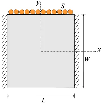
As illustrated in Figure 9, a square bar with L W 1in. is clamped along its left and right surfaces while subjected to a uniform transverse shear stress of S12000 psi on its top surface. The bottom surface is free of loading. These boundary conditions are imposed as





u x L y  (76a)





u

x y W

y

   

 (76b)





z

u

x y W S

y

  

 (76c)

The shear modulus is specified as _{ 12 10 psi}6 _{. The cross section is discretized with a uniform grid}

29

results are shown in Figure 10. The PD theory successfully captures the anti-plane shear deformation, and

this comparison confirms the validity of the implementation for displacement- and stress-type boundary

conditions.

Figure 9. Square bar under anti-plane shear loading.

30

(b)

(c)

Figure 10. Displacement variation across the bar: (a) ordinary state-based PD solution, (b) bond-based PD solution, and (c) FEA solution.

8.2. Bimaterial rectangular bar under anti-plane shear loading

As shown in Figure 11, a bimaterial rectangular bar with L0.2 in. and W 1 in. is clamped along its bottom surface and subjected to a uniform transverse shear stress of S12000 psi on its top surface. The bottom surface is free of any loading. These boundary conditions are imposed as





31





z

u

x L y

x

   

 (77b)





z

u

x y W S

y

  

 (77c)

The shear moduli of the materials are specified as 6

1 12 10 psi

   _and 6

2 6 10 psi

   .The cross section

is discretized with a uniform grid spacing of    x y 0.01 in., resulting in 20 and 100 material points in the x- and in the -y directions, respectively.

Along the vertical axis, the bond-based and ordinary state-based PD displacement variations and their

comparison with the FEA results are shown in Figure 12. The results demonstrate the validity of the PD

modeling of interface conditions. The predictions are in excellent agreement and capture the effect of

dissimilar materials.