Survivor Derivatives: A Consistent Pricing Framework

City, University of London Institutional Repository

Citation

:

Dawson, P., Dowd, K., Cairns, A.J.G. & Blake, D. (2010). Survivor Derivatives: A

Consistent Pricing Framework. Journal Of Risk And Insurance, 77(3), pp. 579-596. doi:

10.1111/j.1539-6975.2010.01356.x

This is the published version of the paper.

This version of the publication may differ from the final published

version.

Permanent repository link:

http://openaccess.city.ac.uk/17995/

Link to published version

:

http://dx.doi.org/10.1111/j.1539-6975.2010.01356.x

Copyright and reuse:

City Research Online aims to make research

outputs of City, University of London available to a wider audience.

Copyright and Moral Rights remain with the author(s) and/or copyright

holders. URLs from City Research Online may be freely distributed and

linked to.

City Research Online:

http://openaccess.city.ac.uk/

[email protected]

SURVIVOR

DERIVATIVES: A CONSISTENT

PRICING

FRAMEWORK

Paul Dawson Kevin Dowd Andrew J. G. Cairns David Blake

ABSTRACT

Survivorship risk is a significant factor in the provision of retirement income. Survivor derivatives are in their early stages and offer potentially significant welfare benefits to society. This article applies the approach developed by Dowd et al. (2006), Olivier and Jeffery (2004), Smith (2005), and Cairns (2007) to derive a consistent framework for pricing a wide range of linear survivor derivatives, such as forwards, basis swaps, forward swaps, and futures. It then shows how a recent option pricing model set out by Dawson et al. (2009) can be used to price nonlinear survivor derivatives, such as survivor swaptions, caps, floors, and combined option products. It concludes by con-sidering applications of these products to a pension fund that wishes to hedge its survivorship risks.

INTRODUCTION

A new global capital market, the Life Market, is developing (see, e.g., Blake, Cairns, and Dowd, 2008) and “survivor pools” (or “longevity pools” or “mortality pools” depending on how one views them) are on their way to becoming the first major new asset class of the twenty-first century. This process began with the securitization of insurance company life and annuity books (see, e.g., Millette et al., 2002; Cowley and Cummins, 2005; Lin and Cox, 2005). But with investment banks entering the growing market in pension plan buyouts, in the United Kingdom in particular, it is only a matter of time before full trading of “survivor pools” in the capital markets begins.1 Recent developments in this market include: the launch of the LifeMetrics

Paul Dawson is at Kent State University. Kevin Dowd is at the Pensions Institute, Cass Business School. Andrew J. G. Cairns is at the Maxwell Institute, Edinburgh and Depart-ment of Actuarial Mathematics and Statistics, Heriot-Watt University. David Blake is at the Pensions Institute, Cass Business School. The authors can be contacted via e-mail: [email protected], [email protected], [email protected], [email protected]. The authors are grateful to Hai Lin and the two anonymous referees for helpful comments.

1_{Dunbar (2006). On February 1, 2010, the Life and Longevity Markets Association (LLMA)}

was established in London by AXA, Deutsche Bank, J.P. Morgan, Legal & General, RBS, and

Index in March 2007; the first derivative transaction, aq-forward contract, based on this index in January 2008 between Lucida, a UK-based pension buyout insurer, and J.P. Morgan (see Coughlan et al., 2007; Grene, 2008); the first survivor swap executed in the capital markets between Canada Life and a group of ILS2and other investors in July 2008, with J.P. Morgan as the intermediary; and the first survivor swap involving a nonfinancial company, arranged by Credit Suisse in May 2009 to hedge the longevity risk in UK-based Babcock International’s pension plan.

However, the future growth and success of this market depends on participants having the right tools to price and hedge the risks involved, and there is a rapidly growing literature that addresses these issues. The present article seeks to contribute to that literature by setting out a framework for pricing survivor derivatives that gives consistent prices—that is, prices that are not vulnerable to arbitrage attack—across all survivor derivatives. This framework has two principal components: one applicable to linear derivatives, such as swaps, forwards, and futures, and the other applicable to survivor options. The former is a generalization of the swap-pricing model first set out by Dowd et al. (2006), which was applied to simple vanilla survivor swaps. We show that this approach can be used to price a range of other linear survivor derivatives. The second component is the application of the option-pricing model set out by Dawson et al. (2009) to the pricing of survivor options such as survivor swaptions. This is a very simple model based on a normally distributed underlying, and it can be applied to survivor options in which the underlying is the swap premium or price, since the latter is approximately normal. Having set out this framework and shown how it can be used to price survivor derivatives, we then illustrate their possible applications to the various survivorship hedging alternatives available to a pension fund.

This article is organized as follows. The “Pricing Vanilla Survivor Swaps” section sets out a framework to price survivor derivatives in an incomplete market setting and uses it to price vanilla survivor swaps. The “Pricing Other Linear Survivor Deriva-tives” section then uses this framework to price a range of other linear survivor deriva-tives: these include survivor forwards, forward survivor swaps, survivor basis swaps, and survivor futures contracts. The “Survivor Swaptions” section extends the pricing framework to price survivor swaptions, caps, and floors, making use of an option pric-ing formula set out in Dawson et al. (2009). The “Hedgpric-ing Applications” section gives a number of hedging applications of our pricing framework, and the “Conclusion” section concludes.

PRICINGVANILLASURVIVORSWAPS

A Model of Aggregate Longevity Risk

It is convenient if we begin by outlining an illustrative model of aggregate longevity risk. Let p(s,t,u,x) be the risk-adjusted probability based on information available atsthat an individual agedxat time 0 and alive at timet≥swill survive to timeu≥ t(referred to as the forward survival probability by Cairns, Blake, and Dowd, 2006). Our initial estimate of the risk-adjusted forward survival probability touis therefore

Swiss Re. The aim is “to support the development of consistent standards, methodologies and benchmarks to help build a liquid trading market needed to support the future demand for longevity protection by insurers and pension funds.”

p(0, 0,u,x), and these probabilities would be used at time 0 to calculate the prices of annuities. We now postulate that, for eachs=1,. . .,t:

p(s,t−1,t,x)= p(s−1,t−1,t,x)b(s,t−1,t,x)ε(s), (1)

where ε (s)> 0 can be interpreted as a survivorship “shock” at time s for agex, although to keep the notation as simple as possible, we do not make the age depen-dence explicit (see also Cairns, 2007, Equation (5); Olivier and Jeffery, 2004; Smith, 2005). For its part,b(s,t−1,t,x) is a normalizing constant, specific to each pair of dates,sandt, and to each cohort, that ensures consistency of prices under our pricing measure.3

It then follows thatS(t), the probability of survival tot, is given by:

S(t)= t

s=1

p(s−1,s−1,s,x)b(s,s−1,s,x)ε(s)= t

s=1

p(0,s−1,s,x) s

u=1

b(u,s−1,s,x)ε(u)

. (2)

We will drop the explicit dependence ofε(.) onsfor convenience. We now consider the survivor shockεin more detail and first note that it has the following properties: 1. A valueε <1 indicates that survivorship was higher than anticipated under the

risk-neutral pricing measure, andε >1 indicates the opposite. 2. Under the risk-neutral pricing measureεhas mean 1.

3. Under our real-world measure, ε has a mean of 1−μ, where μ is the user’s subjective view of the rate of decline of the mortality rate relative to that already anticipated in the initial forward survival probabilitiesp(0, 0,u,x). So, for example, if the user believes that mortality rates are declining at 2 percent per annum faster than anticipated, thenεwould have a mean of 1 – 0.02=0.98.

4. The volatility ofεis approximately equal tostd(qx)/qˆx(see the Appendix), where std(qx) is the conditional one-step-ahead volatility ofqxand ˆqxis its one-step-ahead predictor.

5. It is also apparent from (1) thatεcan also be interpreted as a 1-year ahead forecast error. If expectations/forecasts are rational, then these forecast errors should be independent over time.

We also assume thatεcan be modeled by the following transformed beta distribution:

ε=2y, (3)

where y is beta-distributed. Since the beta distribution is defined over the domain [0,1], the transformed betaεis distributed over domain [0, 2].

3_{The normalizing constants,b(s,t−1,t,x), are known at times– 1. For most realistic cases,}

In order to determine swap premiums under the real-probability measure,4we now calibrate the two parametersνandωof the underlying beta distribution against real-world data to reflect the user’s beliefs about the empirical mortality process. To start with, we know that the mean and variance of the beta distribution areν/(ν+ω) and

υω/[(ν+ω)2(ν +ω+1)], respectively. The mean and variance of the transformed beta are therefore 2ν/(ν+ω) and 4υω/[(ν+ω)2(ν+ω+1)]. If we now set the mean equal to 1 −μ, then it is easy to show that ν =kω, wherek =(1 −μ(x))/(1 +μ (x)). Similarly, we know that the variance of the transformed beta (i.e., the variance of

ε) is approximately equal to var(qx)/qˆ2x, where the variance refers to the conditional one-step-ahead variance. Substituting this into the expression for the variance of the transformed beta and rearranging gives us

var(ε) ≈ var(qx) ˆ q2

x

= 4k

(k+1)2_[ω(k+1)+1] ⇒ω= 4k

(k+1)3_var(ε)−

1 k+1.

In short, given information aboutμand var(ε), we can solve forωandνusing

k= 1−μ

1+μ (4a)

ω= 4k

(k+1)3_var(ε)−

1

k+1 (4b)

ν=kω. (4c)

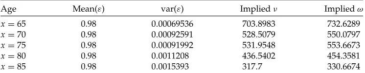
To illustrate how this might be done, Table 1 presents estimates calibrated against recent England and Wales male mortality data for age 65, and assumingμ=2 percent for illustrative purposes, implying that the mean of ε is 0.98. If we letq(t) be our mortality rate for the given age and yeart, and take ˆq(t), our predictor ofq(t), to be equal toq(t −1), thenε(t)=q(t)/q(t −1) and var(ε)=0.00069536.5 The last two columns then show that, to achieve a mean of 0.98 and a variance of 0.00069536, then we needν =703.8983 andω=732.6289. Thus, the model is straightforward to calibrate using historical mortality data. Different users of the model would arrive at a different calibration if they believed that future trend changes in mortality rates for age 65 differed fromμ=2 percent or volatility differed from var(ε)=0.00069536.

4_{Under the risk-neutral pricing measure, by contrast, no calibration is necessary for swap}

purposes as the risk-neutral swap premium is zero.

5_{Mortality rates at timet– 1 obviously represent crude and biased estimators of mortality}

TABLE1

Calibrating the Beta Distribution

Age Mean(ε) var(ε) Impliedν Impliedω x=65 0.98 0.00069536 703.8983 732.6289 x=70 0.98 0.00092591 528.5079 550.0797 x=75 0.98 0.00091992 531.9548 553.6673 x=80 0.98 0.0011208 436.5402 454.3581 x=85 0.98 0.0015393 317.7 330.6674 Notes:The assumed mean in the second column incorporates a subjective believe that mortality will decline at 2 percent per annum. var(ε)≈var(qx)/qˆx2is based on England and Wales male

mortality data over 1961–2005 for 65-year-olds. Impliedνand impliedωare the values that the parameters of the beta distribution must take to ensure that the distribution gives the mean and variances in the previous two columns.

The Dowd et al. (2006) Pricing Methodology

We now explain our pricing methodology in the context of the vanilla survivor swap structure analyzed in Dowd et al. (2006). This contract is predicated on a benchmark cohort of given initial age. On each of the payment dates, t, the contract calls for the fixed-rate payer to pay the notional principal multiplied by a fixed proportion (1+π)H(t) to the floating-rate payer and to receive in return the notional principal multiplied byS(t).H(t) is predicated on the life tables or mortality model available at the time of contract formation and π is the swap premium or swap price that is factored into the fixed-rate payment.6H(t) andπ are set when the contract is agreed and remain fixed for its duration.S(t) is predicated on the actual survivorship of the cohort.

Had the swap been a vanilla interest-rate swap, we could then have used the spot-rate curve to determine the values of both fixed and floating leg payments. We would have invoked zero-arbitrage to determine the fixed rate that would make the values of both legs equal, and this fixed rate would be the price of the swap. In the present context, however, this is not possible because longevity markets are incomplete, so there is no spot-rate curve that can be used to price the two legs of the swap.

Instead, we take the present value of the floating-leg payment to be the expectation of S(t) under the assumed real probability measure. Under our illustrative model, this is given by

E[S(t)]=E

⎡ ⎣t

s=1

p(0,s−1,s,x) s

u=1

b(u,s−1,s,x)ε(u)

⎤

⎦_. (5)

6_{Strictly speaking, the contract would call for the exchange of the difference between (1+}

The premiumπis then set so that the swap value is zero at inception. Hence, ifE[S(t)] denotes each time-texpected floating-rate payment under the our pricing measure, and ifDtdenotes the price at time 0 of a bond paying $1 at timet, then the fair value for ak-period survivor swap requires:

(1+π) k

t=1

DtH(t)= k

t=1

DtE[S(t)] (6)

∴ π=

k

t=1

DtE[S(t)]

k

t=1

DtH(t)

−1. (7)

From this structure, it becomes possible to price a range of related derivatives securi-ties.

Generalizing the Dowd et al. (2006) Pricing Methodology

The pricing model set out earlier can be generalized to a wide range of related deriva-tives. For ease of presentation, we assume that payments due under the derivatives are made annually. We denote the age of cohort members during the life of the derivatives by the following subscripts:

t =their age at the time of the contract agreement;

s =their age at the time of the first payment;

f =their age at the time of the final payment;

n =their age at the time of any given anniversary (t≤n≤f).

Let us also denote:

N =the size of the cohort at aget;

Dn =the discount factor from agetto agen;

Yn =the payment per survivor due at agen(=0 forn<s).

Now note that the present value (at timet) of a fixed payment due at timenis

(1+π)NYnDnH(n). (8)

(1+π)N f

n=t+1

YnDnH(n), (9)

which—conditional onπ—can be determined easily at timetfrom the spot-rate curve. Following the same approach as with the vanilla survivor swap, the present value of the floating rate leg is

N×E

⎡ ⎣ f

n=t+1

YnDnS(n)

⎤ ⎦ ₌N

f

n=t+1

YnDnE[S(n)]. (10)

Since a swap has zero value at inception, we then combine (9) and (10) to calculate a premium,π_s,f, for any swap-type contract, valued at timet, whose payments start at agesand finish at agef . This premium is given by

πs,f = f

n=t+1

YnDnE[S(n)]

f

n=t+1

YnDnH(n)

−1. (11)

PRICINGOTHERLINEAR SURVIVORDERIVATIVES

We now use the pricing methodology outlined in the previous section to price some key linear survivor derivatives.

Survivor Forwards

Just as an interest-rate swap is essentially a portfolio of FRA contracts, so a survivor swap can be decomposed into a portfolio of survivor forward contracts. Consider two parties, each seeking to fix payments on the same cohort of 65-year-old annuitants. The first enters into ak-year, annual-payment, pay-fixed swap as described earlier, and with premium,π. The second enters into a portfolio ofkannual survivor forward contracts, each of which requires payment of the notional principal multiplied by (1+πn)H(n) and the receipt of the notional principal multiplied byS(n),n=1,2,. . .k. Note that in this second case, πn differs for each n. Since the present value of the commitments faced by the two investors must be equal at the outset, it must be that:

(1+π) k

n=1

DnH(n)= k

n=1

∴ π = k

n=1

DnH(n)πn k

n=1

DnH(n)

. (13)

Hence, it follows thatπin the survivor swap must be equal to the weighted average of the individual values ofπnin the portfolio of forward contracts, in the same way that the fixed rate in an interest-rate swap is equal to the weighted average of the forward rates.

Forward Survivor Swaps

Given the existence of the individual values ofπnin the portfolio of forward contracts, it becomes possible to price forward survivor swaps. In such a contract, the parties would agree at time 0 the terms of a survivor swap contract that would commence at some specified time in the future. Not only would such a contract meet the needs of those who are committed to providing pensions in the future, but it could also serve as the hedging vehicle for survivor swaptions, as shown later.

The pricing of such a contract would be quite straightforward. As shown earlier, the position could be replicated by entering into an appropriate portfolio of forward contracts. Thus,πforwardswap—the risk premium for the forward swap contract—must equal the weighted average of the individual values of πn used in the replication strategy.πforwardswapcan then be derived directly from Equation (11).

Basis Swaps

Dowd et al. (2006) also discuss, but do not price, a floating-for-floating swap, in which the two counterparties exchange payments based on the actual survivorships of two different cohorts. Following practice in the interest-rate swaps market, such contracts should be called basis swaps. Their approach shows how such contracts could be priced. First, consider two parties wishing to exchange the notional principal7 multi-plied by the actual survivorship of cohortsjandk. Assume equal notional principals and denote the risk premiums and expected survival rates for such cohorts by πi and π_k and by H_j(n) and H_k(n), respectively. Given the existence of vanilla swap contracts on each cohort, the present values of the fixed leg of each such contract will be (1+πj) _nf₌₁DnHj(n) and (1+πk) _nf₌₁DnHk(n), respectively, and the no-arbitrage argument shows that these must also be the present values of the expected floating-rate legs. It is then possible to calculate, with certainty, an exchange factor,κ,

7_{Following practice in the interest rate swaps market, we avoid constant reference to the}

such that

1+πj

f

n=1

DnHj(n)=κ(1+πk) f

n=1

DnHk(n) (14)

and, hence

κ=

1+πj

f

n=1

DnHj(n)

(1+πk) f

n=1

DnHk(n)

, (15)

from which it follows that the fair value in a floating-for-floating basis swap requires one party to make payments determined by the notional principal multiplied by S_j(n) and the other party to make payments determined by the notional principal multiplied byκS_k(n);κ is determined at the outset of the basis swap and remains fixed for the duration of the contract.

The same approach can be used to price forward basis swaps, in which case, following earlier analysis,κis given by

κ =

1+πj f

n=s

DnHj(n)

(1+πk) f

n=s

DnHk(n)

. (16)

Cross-Currency Basis Swaps

We turn now to price a cross-currency basis swap, in which the cohort-jpayments are made in one currency and the cohort-kpayments in another. The single currency floating-for-floating basis swap analyzed in the preceding subsection required the cohort-jpayer to payS_j(n) at each payment date and to receiveκS_k(n). Now consider a similar contract in which the cohort-j payments are made in currency jand the cohort-kpayments made in currencyk. Assume the spot exchange rate between the two currencies isFunits of currencykfor each unit of currencyj.8

From the arguments above, we can determine the present value of each stream—(1+πj) _nf₌₁DnHj(n) and (1+πk) _nf₌₁DnHk(n), respectively, each ex-pressed in their respective currencies. Multiplying the latter by F then expresses the value of the cohort-kstream in units of currency j. The standard requirement

8_{In foreign exchange markets parlance, currencyjis the base currency and currencykis the}

that the two streams have the same value at the time of contract agreement is again achieved by determining an exchange factor,κFX. In the present case, this exchange factor,κFXis given by:

(1+πj) f

n=1

DnHj(n)=κFXF(1+πk) f

n=1

DnHk(n) (17)

∴ κFX=

(1+πj) f

n=1

DnHj(n)

F(1+πk) f

n=1

DnHk(n)

. (18)

Thus, in the case of a floating-for-floating cross-currency basis swap, on each payment date,n, one party will make a payment of the notional principal multiplied bySj(n) and receive in return a payment ofκFX Sk(n). Each payment will be made in its own currency, so that exchange rate risk is present. However, in contrast with a cross-currency interest-rate swap, there is no exchange of principal at the termination of the contract, so the exchange rate risk is mitigated.

The same procedure is used for a forward cross-currency basis swap, except that the summation in Equations (17) and (18) above is fromn=stof rather than from n =1 tof. Since the desire is to equate present values, it should be noted that the spot exchange rate,F, is applied in this equation rather than the forward exchange rate.9

Futures Contracts

The wish to customize the specification of the cohort(s) in the derivative contracts described earlier implies trading in the over-the-counter (OTC) market. However, an exchange-traded instrument offers attractions to many, especially in light of proposed regulatory intervention in derivatives markets.10As shown earlier, the uncertainty in survivor swaps is captured in factorπ, and a futures contract withπas the underlying asset would serve a useful function both as a hedging vehicle and for investors who wished to achieve exchange-traded exposure to survivor risk, in much the same way as the Eurodollar futures contract is based on 3-month Eurodollar LIBOR.

Thus, if the notional principal were $1 million and the time frame were 1 year, a long position in a December futures contract at a price of π = 3 percent would

9_{The foreign exchange risk could be eliminated by use of a survivor swap contract in which}

the payments in one currency are translated into the second currency at a predetermined exchange rate, similar to the mechanics of a quanto option. Derivation of the pricing of such a contract is left for future research.

10_{See Kopecki and Leising (2009) and Henson and Shah (2009) for discussions of proposed U.S.}

notionally commit the holder to pay $1.03 million multiplied by the expected size of the cohort surviving and to receive $1 million multiplied by the actual size. This is a notional commitment only: in practice, the contracts would be cash-settled, so that if the spot value ofπ at the December expiry, which we denoteπexpiry, were 4 percent, the investor would receive a cash payment of $10,000, that is, (4–3) percent of $1 million.11

The precise cohort specification would need to be determined by research among likely users of the contracts. Too many cohorts would spread the liquidity too thinly across the contracts; too few cohorts would lead to excessive basis risk.

Determination of the settlement price at expiry might be achieved by dealer poll. Such futures contracts could be expected to serve as the principal driver of price discovery in the Life Market, with dealers in the OTC market using the futures prices to inform their pricing of customized survivor swap contracts.

SURVIVOR SWAPTIONS

Where there is demand for linear payoff derivatives, such as swaps, forwards, and futures, there is generally also demand for option products. An obvious example is a survivor swaption contract.

Specification of Swaptions

The specification of such options is quite straightforward. Consider a forward sur-vivor swap, described earlier, with premiumπforwardswap. A swaption would give the holder the right but not the obligation to enter into a swap on specified terms. Clearly, the exercise decision would depend on whether the market rate of theπ at expiry for such a swap was greater or less than π_forwardswap. Thus, in the case described,

πforwardswapis the strike price of the swaption. Of course, the strike price of the option does not have to beπ_forwardswapbut can be any value that the parties agree. However, usingπ_forwardswapas an example shows how put-call12parity applies to such swap-tions. An investor who purchases a payer swaption, at strike priceπ_forwardswap, and writes a receiver swaption with an identical specification has synthesized a forward survivor swap. Since such a contract could be opened at zero cost, it follows that a synthetic replication must also be available at zero cost. Hence, the premium paid for the payer swaption must equal the premium received for the receiver swaption.

The exercise of these swaptions could be settled either by delivery (i.e., the parties enter into opposite positions in the underlying swap) or by cash, in which case the writer pays the holder Max[0,φπexpiry−φπstrike]N _nf₌₁Dexpiry,nYnH(n) withφ set

11_{Recall, however, thatπcan take values between –1 and 1. Since negative values are rare for}

traded assets, this raises the issue of whether user systems are able to cope. To avoid such problems, the market forπ futures contracts could either be quoted as (1+π), withπ as a decimal figure, or follow interest-rate futures practice and be quoted as (100−π) withπ expressed in percentage points.

12_{In swaptions markets, usage of terms such as put and call can be confusing. Naming such}

as +1 for payer swaptions and −1 for receiver swaptions, πexpiry representing the market value ofπat the time of swaption expiry,π_strikerepresenting the strike price of the swaption, andDexpiry,nrepresenting the price at option expiry of a bond paying 1 at timen.13

Pricing Swaptions

Our survivor swaptions are specified on the swap premium π as the underlying, and this raises the issue of how π is distributed. In a companion paper, Dawson et al. (2009) suggest that π should be (at least approximately) normal, and they report Monte Carlo results that support this claim.14 We can therefore state that

π is approximately N(π_forwardswap, σ2), where σ2 is expressed in annual terms in accordance with convention. Normally distributed asset prices are rare, because such a distribution permits the asset price to become negative. In the case ofπ_forwardswap, however, negative values are perfectly feasible.

Dawson et al. (2009) derive and test a model for pricing options on assets with normally distributed prices and application of their model to survivor swaptions gives the following formulae for the swaption prices:

Ppa yer=e−rτ((πforwardswap−πstrike)N(d)+σ √

τN(d)) (19)

Preceiver=e−rτ((πstrike−πforwardswap)N(−d)+σ √

τN(d)) (20)

d= πforwardswap−πstrike

σ√τ . (21)

In (19)–(21) above,rrepresents the interest rate,τthe time to option maturity, andσthe annual volatility of the returns ofπforwardswap.N(d) is the standard normal cumulative distribution function of d, with d ∼N(0, 1).N(d) is the corresponding probability

13_{Under Black-Scholes (1973) assumptions, interest rates are constant, so that}

N nf=1Dexpir y,nYnH(n) is known from the outset. Let us call this the settlement sum.

Fol-lowing the approach in footnote 7, we can dispense with constant repetition of the settlement sum by expressing option values in percentages and recognising that these can be turned into a monetary amount by multiplying by the settlement sum.

14_{More precisely, the large Monte Carlo simulations (250,000 trials) across a sample of}

dif-ferent sets of input parameters reported in Dawson et al. (2009) suggest thatπforwardswap is

close to normal but also reveal small but statistically significant nonzero skewness values. Furthermore, while excess kurtosis is insignificantly different from zero when drawing from beta distributions with relatively low standard deviations, the distribution ofπforwardswapis

density function. Apart from replacing geometric Brownian motion with arithmetic Brownian motion, this valuation model is predicated on the standard Black-Scholes (1973) assumptions, including,inter alia, continuous trading in the underlying asset. Naturally, we recognize that, at present, no such market exists.

The use of this model in practice would, therefore, inevitably involve some degree of basis risk. This arises, in part, because it is unlikely that a fully liquid market will ever be found in the specific forward swap underlying any given swaption. A liquid market in theπfutures described earlier would mitigate these problems, how-ever.15 Furthermore, survivor swaption dealers will likely need to hedge positions in swaptions on different cohorts, which will be self-hedging to a certain extent and so reduce basis risk. We could also envisage option portfolio software that would translate some of the remaining residual risk into futures contract equivalents, thus dictating (and possibly automatically submitting) the orders necessary for maintain-ing delta-neutrality.

Most liquid futures markets create a demand for futures options, and this leads to the possibility of π futures options. Pricing such contracts is also accomplished in (19)–(20) above. All that is necessary is to substitute π_futures for π_forwardswap as the value of the optioned asset.

Survivor Caps and Floors

The parallels with the interest rate swaps market can be carried still further. In the interest rate derivatives market, caps and floors are traded, as well as swaptions. These offer more versatility than swaptions, since each individual payment is optioned with a caplet or a floorlet, while a swaption, if exercised, determines a single fixed rate for all payments. The extra optionality comes at the expense of a significantly increased option premium, however. Similar caplets and floorlets can be envisaged in the market for survivor derivatives and can be priced using (19) and (20) with theπvalue for the survivor forward contract serving as the underlying in place ofπ_forwardswap.

HEDGINGAPPLICATIONS

In this section, we consider applications of the securities presented earlier. By way of example, we consider a pension fund with a liability to pay $10,000 annually to each survivor of a cohort of 10,000 65-year-old males. Using the same life tables as Dowd et al. (2006), and assuming a yield curve flat at 3 percent, the present value of this liability is approximately $1.41 billion and the pension fund is exposed to survivorship risk. We consider several strategies to mitigate this risk. In pricing the various securities applied, we use the models presented earlier in this article and, in accordance with Table 1, use values ofν =703.8983 andω=732.6289 for the two parameters specifying the beta distribution used to modelεin (3) above.

The first hedging strategy that the fund might undertake is to enter into a 50-year survivor swap. Using the framework of this article gives a swap rate of 10.39 per-cent. Entering a pay-fixed swap at this price would remove the survivor risk entirely

15_{Given a variety of cohorts, basis risk could be a problem, but as noted earlier, an important}

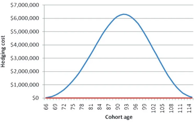
FIGURE1

Distribution of the Cost of Hedging Over Cohort Ages

from the pension fund but increase the present value of its liabilities to approxi-mately $1.56 billion ($1.41 billion×1.1039). The cost of hedging in this case is thus $0.15 billion.

The second hedging strategy has the pension fund choosing to accept survivor risk for the next 5 years and entering into a forward swap today to hedge survivor risk from age 71 onward. The value ofπ in this case is 15.07 percent. The $1.41 billion present value of the pension fund’s liabilities can be broken down into $0.44 billion for the first 5 years and $0.97 billion for the remaining 45 years. Opening a pay-fixed position in this forward swap would again raise the present value of the pension fund’s liabilities to $1.56 billion ($0.44 billion+$0.97 billion×1.1507). From this, it can be seen that the cost of hedging just the first 5 years of the pension fund’s liabilities is close to zero. In fact, the fairπvalue for such a swap is just 0.16 percent which, on a present value of $0.44 billion, amounts to less than $1 million.

These three hedging strategies fix the commitments of the pension fund, either for the entire period of survivorship or for all but the first 5 years, and this means that the fund would have no exposure to any financial benefits from decreasing survivorship during the hedged periods. These benefits could, however, be obtained by our fourth hedging strategy, namely, a position in a 5-year payer swaption. Again, the fund would accept survivor risk for the first 5 years but would then have the right, but not the obligation, to enter a pay-fixed swap on pre-agreed terms. Using the same beta parameters as above, the annual volatility of the forward contract is 4.36 percent and the premium for an at-the-money forward swaption is 3.35 percent. Applying the swaption formula, the pension fund would pay an option premium of approximately $32 million to gain the right but not the obligation to fix the payments at aπ rate of 15.07 percent thereafter. If survivorship declines, the fund will not exercise the option and will have lost merely the $32 million swaption premium but then reaps the benefit of the decline in survivorship.

Rather more optionality could be obtained through a survivor cap rather than a survivor swaption. As described earlier, this is constructed as a portfolio of options on survivor forwards. The expiry value of each option isNYH(n)Max[0, π_settlement −πstrike], in whichπsettlement refers to the value ofπ prevailing for that particular payment at the time,n, at which the settlement is due. Its value at expiry is simply S(n)/H(n) – 1. Thus, on each payment date,n, the pension fund holding a survivor cap effectively pays NY(1 +Min[πsettlement,πstrike])H(n) and receivesNYS(n) in re-turn, with this receipt designed to match its liability to its pensioners. This extra optionality comes at a price: it was noted earlier that the option premium for a 5-year survivor swaption, at strike price 15.07 percent, with our standard parameters, was approximately $32 million. The equivalent survivor cap (in which the pension fund again accepts survivor risk for the first 5 years but hedges it with a survivor cap again struck at 15.07 percent for the remaining 45 years) would carry a premium of approximately $129 million.

Our next hedging strategy is a zero-premium collar. Again using the same beta parameters, the premium for a payer swaption with a strike price of 16.5 percent is 2.77 percent or about $27 million. The same premium applies to a receiver swaption with a strike price of 12.72 percent. Thus, a zero-premium collar can be constructed with a long position in the payer swaption financed by a short position in the receiver swaption. With such a position, the pension fund would be hedged, for a premium of zero, against the price of a 45-year swap rising above 16.5 percent by the end of 5 years and would enjoy the benefits of the swap rate falling over the same period, but only as far as 12.72 percent.

at zero premium, complete protection against the survivor premium rising above 16.5 percent, and unlimited participation, albeit at about 12c on the dollar, if the survivor premium turns out to be less than this.

The hedging strategies presented so far in this section serve to transfer the survivor risk embedded in a pension fund to an outside party. In all cases, this is done at a cost: either an explicit financial cost or, in the case of the zero-premium option structures, at the willingness to forego some of the financial benefits of falling survivorship, that is, at an opportunity cost. A quite different alternative that avoids these costs is simply for the pension fund to diversify its exposure. Using a basis swap or a cross-currency basis swap, the pension fund could swap some of its exposure to the existing cohort for an exposure to a different cohort (either in its domestic economy or overseas). Hence, in return for receiving cash flows to match some of its obligations to its own pensioners, it would assume liability for paying according to the actual survivorship of a different cohort. As the derivations of Equations (15) and (17) show, this does not change the value of the pension fund’s liabilities but, assuming less than perfect correlation between the survival rates of the two cohorts, enables the pension fund to enjoy the benefits of diversification.

CONCLUSION

This article develops a consistent pricing framework applicable across a wide variety of survivor derivatives. Further developments can be expected. First, as mentioned earlier, quanto features could be incorporated in cross-currency products to eliminate currency risk. Next, barrier features might also be anticipated. For example, a pension fund might be quite willing to forego protection against increasing survivorship in the event of a flu pandemic and would buy a payer swaption that knocks out if mortality rises above a predetermined threshold. Such a payer swaption would specify a low value ofπas the knock-out threshold. Alternatively, such a fund might seek protection contingent on a major breakthrough in the treatment of cancer and would thus buy a payer swaption, which knocks in if survivorship rises above a predetermined threshold. Such a payer swaption would specify a high value ofπas the knock-in threshold.

Survivorship is a risk of considerable importance to developed economies. It is sur-prising that the market has been so slow to develop derivative products to manage such risk. However, parallels with other markets seem apposite: once the initial prod-ucts were launched, the growth in these markets was rapid, and as of the time of writing (mid-2009), we are already witnessing increasingly rapid developments in the longevity swaps space.

APPENDIX

This appendix shows that volatility ofstd(ε)≈std(qx)/qx.ˆ

Proof: Letp₁= p(s,t−1,t,x) and p₀=p(s−1,t−1,t,x). Sinceb(.)≈1, then (1) in the main text implies

p1≈ p₀ε

Now letq1andq0be the mortality rates corresponding to p1and p0. We know that

log(p1)≈ −q1and log(p0)≈ −q0, so

var(q1)≈q₀2×var(ε) ⇒ std(ε)≈ std(q1)

q0

orstd(qx) ˆ qx

where ˆqx=1−p(s−1,t−1,t,x) is the one-step-ahead predictor ofqx=1−p(s,t−

1,t,x). Q.E.D.

REFERENCES

Black, F., and M. Scholes, 1973, The Pricing of Options and Corporate Liabilities, Journal of Political Economy, 81: 637-654.

Blake, D., A. J. G. Cairns, and K. Dowd, 2008, The Birth of the Life Market,Asia-Pacific Journal of Risk and Insurance, 3(1): 6-36.

Cairns, A. J. G., 2007, A Multifactor Generalisation of the Olivier-Smith Model for Stochastic Mortality, in: Proceedings of the First IAA-LIFE Colloquium (Stockholm).

Cairns, A. J. G., D. Blake, and K. Dowd, 2006, Pricing Death: Frameworks for the Evaluation and Securitization of Mortality Risk, ASTIN Bulletin, 36: 79-120.

Coughlan, G., D. Epstein, A. Sinha, and P. Honig, 2007, q-Forwards: Derivatives for Transferring Longevity and Mortality Risks(London: J.P. Morgan Pension Advisory Group). World Wide Web: www.lifemetrics.com (accessed March 7, 2010).

Cowley, A., and J. D. Cummins, 2005, Securitization of Life Insurance Assets and Liabilities,Journal of Risk and Insurance, 72: 193-226.

Dawson, P., K. Dowd, D. Blake, and A. J. G. Cairns, 2009, Options on Normal Under-lyings With an Application to the Pricing of Survivor Swaptions,Journal of Futures Markets, 29: 757-774.

Dowd, K., D. Blake, A. J. G. Cairns, and P. Dawson, 2006, Survivor Swaps,Journal of Risk and Insurance, 73: 1-17.

Dunbar, N., 2006, Regulatory Arbitrage, Editor’s Letter,Life & Pensions, April. Grene, S., 2008, Death Data Drive New Market,Financial Times, March 17.

Henson, C., and N. Shah, 2009, European Commission Outlines Derivatives Revamp Plan,Wall Street Journal, July 3.

Kopecki, D., and M. Leising, 2009, Derivatives Get Second Look From US Congress That Didn’t. World Wide Web: http://bloomberg.com/apps/news? pid=20670001&sid=aTZhIZJYCeS8 (accessed March 7, 2010).

Lin, Y., and S. H. Cox, 2005, Securitization of Mortality Risks in Life Annuities,Journal of Risk and Insurance, 72: 227-252.

Olivier, P., and T. Jeffery, 2004, Stochastic Mortality Models, in:Proccedings of the Pre-sentation to the Society of Actuaries of Ireland. Available at: http://web.actuaries.ie/ Events%20and%20Papers/Events%202004/2004-06-01 PensionerMortality/2004-10-20 Stochastic%20MortalityModelling/2004-PensionerMortality/2004-10-20 Stochastic

%20Mortality%20Model.pdf (accessed March 7, 2010).