Testing supervised classifiers based on non-negative matrix factorization to musical instrument classification

      

City, University of London Institutional Repository

Citation

:

Benetos, E., Kotropoulos, C., Lidy, T. and Rauber, A. (2006). Testing supervised

classifiers based on non-negative matrix factorization to musical instrument classification.

Paper presented at the EUSIPCO 2006: 14th European Signal Processing Conference, 4 - 8

Sep 2006, Florence, Italy.

This is the unspecified version of the paper.

This version of the publication may differ from the final published

version.

Permanent repository link:

http://openaccess.city.ac.uk/3242/

Link to published version

:

Copyright and reuse:

City Research Online aims to make research

outputs of City, University of London available to a wider audience.

Copyright and Moral Rights remain with the author(s) and/or copyright

holders. URLs from City Research Online may be freely distributed and

linked to.

TESTING SUPERVISED CLASSIFIERS BASED ON NON-NEGATIVE MATRIX

FACTORIZATION TO MUSICAL INSTRUMENT CLASSIFICATION

Emmanouil Benetos Constantine Kotropoulos

Thomas Lidy and Andreas Rauber

Aristotle Univ. of Thessaloniki Dept. of Informatics

Box 451, Thessaloniki 541 24, Greece

E-mail:{empeneto, costas}@aiia.csd.auth.gr

Vienna University of Technology

Dept. of Software Technology and Interactive Systems Favoritenstrasse 9-11/188, A-1040 Vienna, Austria

E-mail:{lidy, rauber}@ifs.tuwien.ac.at

ABSTRACT

In this paper, a class of algorithms for automatic classifica-tion of individual musical instrument sounds is presented. Two feature sets were employed, the first containing percep-tual features and MPEG-7 descriptors and the second con-taining rhythm patterns developed for the SOMeJB project. The features were measured for 300 sound recordings con-sisting of 6 different musical instrument classes. Subsets of the feature set are selected using branch-and-bound search, obtaining the most suitable features for classification. A class of supervised classifiers is developed based on the non-negative matrix factorization (NMF). The standard NMF method is examined as well as its modifications: the lo-cal and the sparse NMF. The experiments compare the two feature sets alongside the various NMF algorithms. The re-sults demonstrate an almost perfect classification for the first set using the standard NMF algorithm (classification error 1.0%), outperforming the state-of-the-art techniques tested for the aforementioned experiment.

1. INTRODUCTION

The need for musical content analysis arises in different con-texts and has many practical applications, mainly for auto-matic music transcription, effective data organization and an-notation in multimedia databases, and internet search. Au-tomatic musical instrument classification is the first step in developing such applications. It is a research area which can also be applied to general sound recognition tasks. How-ever, despite the massive research which has been carried out in the automatic speech recognition, limited work has been done on musical content identification.

The experiments carried out so far can be broadly clas-sified into two categories: classification of isolated instru-ment tones and classification of sound seginstru-ments. Classifiers using isolated tones have a limited use in a practical appli-cation, while sound segment classifiers could be effectively used in music retrieval systems. Using 2-second segments and employing a back propagation neural network for 7 in-strument classes, a classification accuracy of 99% is reported in [7]. Samples were extracted from the MIS Database from UIOWA [1] that is used in this paper as well. In addition, Synak et al [8] used MPEG-7 temporal descriptors and var-ious spectral features for sound segments consisting of 18 instrument classes and developed 2 classifiers. The first clas-sifier uses the k-NN algorithm, while the second one uses

This work has been supported by the FP6 European Union Network of Excellence MUSCLE “Multimedia Understanding through Semantics, Computation, and Learning” (FP6-507752).

decision rules based on rough sets theory. They achieve a recognition rate of 68.4% at best.

Non-negative matrix factorization (NMF) is a subspace method for basis decomposition [4]. Its various modifica-tions have been used in several classification experiments, where the training procedure is performed by applying an NMF algorithm to a data matrix containing the training vec-tors of all the available classes. This technique results to an unsupervised training approach. NMF classification exper-iments report encouraging results compared to other unsu-pervised classifiers, but also indicate that a suunsu-pervised NMF classification approach is also needed to obtain comparable results with other supervised classifiers.

In this work, the problem of automatically classifying musical instrument segments is addressed. Recordings from the UIOWA database [1] were used that form 6 instrument classes. Two different feature sets were employed, the first covering perceptual descriptors as well as spectral descrip-tors defined by the MPEG-7 audio standard [2]. The first and second moments of the features were considered, creating a feature set of 41 dimensions as explained in Section 4.2. The second feature set uses rhythm patterns developed in the SOMeJB project, which are used for music archives organi-zation [14]. The resulting feature dimension was 1440 for each recording. Branch-and-bound selection was applied to the feature set in order to select the subset that maximizes the classification accuracy [11]. The audio files were split into a training set and a test set using 70% of the available data for training and the remaining 30% for testing. For clas-sification, NMF is used by training individually a classifier for each class and projecting the test data onto each trained class matrix. The class label of each test recording is deter-mined by using the cosine similarity measure (CSM). Sev-eral variants of the NMF algorithm were employed, such as the standard NMF method, the local, and the sparse NMF. The results indicate that the 6-feature subset from the first feature set and the standard NMF algorithm yields a correct classification rate of 99.0%, outperforming the traditional un-supervised NMF classification methods and other statistical model-based classifiers employed for the aforementioned ex-periment [9].

[image:3.595.58.281.80.191.2]

Table 1: List of feature set 1. 1 Zero-Crossing Rate 2 Delta Spectrum (Spectrum Flux) 3 Spectral Rolloff Frequency 4 Mel-Frequency Cepstral Coefficients 5 MPEG-7 AudioSpectrumCentroid 6 MPEG-7 AudioSpectrumEnvelope 7 MPEG-7 AudioSpectrumSpread 8 MPEG-7 AudioSpectrumFlatness 9 MPEG-7 AudioSpectrumProjection Coefficients

2. FEATURE EXTRACTION

In an audio classification system, the intention of the feature extraction step is to adequately and sufficiently describe the semantics of the audio content. In our approach, two feature sets were created, the first combining features describing the temporal and spectral sound structure. The second set is a time-invariant representation of fluctuation patterns on criti-cal bands according to perception of the human auditory sys-tem.

2.1 Feature Set 1

In the first set, a combination of features originating from general audio data classification and the MPEG-7 audio framework is used. The complete list of extracted features is presented in Table 1.

The scalar features 1-3 are proposed in systems con-cerning general audio data (GAD) classification and speech recognition. They can be treated as a short-term descrip-tion of the textural shape of the audio segments. The mel-frequency cepstral coefficients (MFCCs) form a feature vec-tor. They are widely used in audio processing applications providing a description of the spectral shape of the audio sig-nal. 13 MFCCs were used for each audio frame of 10 msec duration. The features 5-8 are proposed by the MPEG-7 au-dio standard [2]. They belong to the basic spectral descrip-tors category. As 9th feature we used the projection coeffi-cient to a single basis. AudioSpectrumProjection coefficoeffi-cients are part of the MPEG-7 spectral basis descriptors.

2.2 Feature Set 2

Rhythm Patterns form the second feature set, developed as part of the SOMeJB project [12], [13], [14], [15] whose main focus is the description and automatic organization of mu-sic archives containing different styles or genres of mumu-sic. The feature set is also suitable to differentiate between vari-ous classes of instruments, the reason being, that the feature set not only focuses on the description of rhythm in narrow sense, but also on fluctuations within the different pitch re-gions.

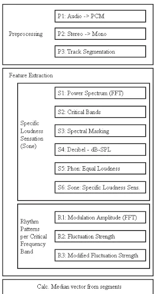
The algorithm for extracting the Rhythm Patterns is a two stage process: First, from the audio spectrum the specific loudness sensation according to the human auditory system is computed. Then, those values are transformed into a time-invariant domain resulting in a representation of modulation amplitudes per modulation frequency on several frequency regions (critical bands). In the following, we will give an outline of all the steps involved in the feature extraction pro-cess. An overview of the procedure is depicted in Figure 1.

The algorithm processes audio tracks in standard digi-tal PCM format with 44.1 kHz sampling frequency as in-put. Each audio track is segmented into pieces of 6 seconds length. A short time Fast Fourier Transform (STFT) is ap-plied to retrieve the energy per frequency band (the spec-trum) every 11.5 ms, resulting in a spectrogram of the 6 sec-ond segment. The frequency bands of the spectrogram are summarized to 24 critical bands, according to the Bark scale [16].

Figure 1: Block diagram of Rhythm Pattern extraction.

The data is then transformed into the logarithmic decibel scale. For transformation into the unit Phon the algorithm incorporates the so-called equal-loudness curves, which ac-count for different loudness sensation of humans in differ-ent frequency regions. Afterwards a conversion into the unit Sone is done, reflecting the specific loudness sensation of the human auditory system according to loudness levels. At this point, we retrieved the specific loudness sensation over time on 24 critical frequency bands. Still, we have a time-dependent signal, although reduced to 511 sample values at the time axis due to the window size in the STFT.

[image:3.595.348.506.181.480.2]

au-dible tones are perceivable. The algorithm captures modula-tion frequencies up to 43 Hz, however the algorithm is set to cut off the information above a modulation frequency of 10 Hz. Subsequently, modulation amplitudes in that range are weighted according to a function of human sensation depend-ing on modulation frequency, accentuatdepend-ing values around 4 Hz, followed by the application of a gradient filter and Gaus-sian smoothing.

The final feature vector contains a time-invariant repre-sentation of fluctuation strength according to human sensa-tion between 0.168 Hz and 10 Hz of modulasensa-tion frequency on 24 critical frequency band regions. A feature vector for each 6 second segment of a piece of audio is calculated. In order to summarize the characteristics of an entire piece of audio (especially music) we average the feature vectors de-rived from its segments by computing the median.

3. NON-NEGATIVE MATRIX FACTORIZATION

Non-negative matrix factorization (NMF) has been proposed as a novel subspace method in order to obtain a parts-based representation of objects by imposing non-negative constraints [4]. The problem addressed by NMF is as fol-lows. Given a non-negativen×mdata matrixV(consisting ofmvectors of dimensionsn×1), it is possible to find non-negative matrix factorsWandHin order to approximate the original matrix:

V≈WH (1)

where then×rmatrixWcontains the basis vectors and the

r×mmatrixHcontains in its columns the weights needed to properly approximate the corresponding column of matrix

Vas a linear combination of the columns ofW. Usually, the component numberris chosen so that(n+m)r<nm, thus resulting in a compressed version of the original data matrix. To find an approximate factorization in (1), a suitable ob-jective function has to be defined. The generalized Kullback-Leibler (KL) divergence between V and WH is the most frequently used objective function. Various algorithms that incorporate additional constraints in deriving (1) have been proposed that are briefly reviewed subsequently.

3.1 Standard NMF

The standard NMF enforces the non-negativity constraints on matricesWandH. Thus, a data vector can be formed by an additive combination of basis vectors. The proposed cost function is the generalized KL divergence:

D(V||WH) = n

∑

i=1

m

∑

j=1

[v_{i j}logvi j

y_{i j}−vi j+yi j] (2)

where WH=Y= [y_{i j}]. D(V||WH) reduces to KL diver-gence when ∑ni=1∑

m

j=1vi j=∑ n i=1∑

m

j=1yi j=1. NMF

fac-torization is defined then as the solution of the optimization problem:

min

W,H D(V||WH) sub ject to W,H≥0, n

∑

i=1

w_{i j}=1∀j (3)

whereW,H≥0 means that all elements of matricesWand

Hare non-negative. The above optimization problem can be solved by using the iterative multiplicative rules [4].

3.2 Local NMF (LNMF)

Aiming to impose constraints concerning spatial locality and consequently revealing local features in the data matrixV, LNMF incorporates 3 additional constraints into the standard NMF problem: 1) Minimize the number of basis components representingV. 2) The different bases should be as orthog-onal as possible. 3) Retain the components giving most im-portant information. The above constraints are expressed in the following LNMF cost function:

D(V||WH) = n

∑

i=1

m

∑

j=1

[v_{i j}logvi j

y_{i j}−vi j+yi j]

+ α

∑

r

i=1

r

∑

j=1

u_{i j}−β

r

∑

i=1

r

∑

j=1

q_ii (4)

where α,β are constants, WTW=U= [u_{i j}], and HHT = Q= [q_{i j}]. The minimization is similar to the one used in NMF (3) and a local solution can be found by using 3 update rules, whereαandβare considered equal to 1 [5].

3.3 Sparse NMF (SNMF)

Inspired by NMF and sparse coding, the aim of SNMF is to impose constraints that can reveal local sparse features on data matrixV. The following cost function is optimized for SNMF:

D(V||WH) = n

∑

i=1

m

∑

j=1

[v_{i j}logvi j

y_{i j}−vi j+yi j]+λ

m

∑

j=1

||hj||l (5)

whereλ is a positive constant and||h_j||_lthel-norm of the j -th column ofH. An SNMF factorization is defined as in (3), including also that∀i||wi||l=1. In SNMF, the sparseness is

measured by a linear activation penalty, the minimuml-norm of the column ofH. A local solution of the minimization problem (5) can be obtained by the update rules proposed in [6].

3.4 Supervised NMF Classification

The major drawback of unsupervised NMF classification presented in [9] is the manner of learning parts-based pat-terns from the data, since no information about the class dis-crimination is incorporated into the NMF training procedure. In addition, the initial random values of matricesWandH

can affect the convergence of the algorithm, as the value of NMF objective function defined in (2) may result in a local minimum, thus not yielding in an appropriate factorization.

In this paper, a supervised classifier where the NMF training procedure is performed for each data class individu-ally is applied, thus resulting in a pair of matricesWandH

for each class:

V_i=W_iH_i, i=1,2,···,N (6)

whereNis the number of different classes,V_ithe data matrix of classi. The number of components used for training each class is given by:

r_i=

n_im_i n_i+m_i

(7)

where the training of each class is performed individually, by using a set of training data representing the respective class in the absence of counter-examples [10].

vt

. . .

h_t(2)

h_t(N)

.

. .

. . .

W₁

W₂

W_N

h(1)_t H₁

H₂

H_N

arg max

h(_ti)=W†_i·vt

CSM_N CSM₁

[image:5.595.55.290.117.240.2]

CSM₂

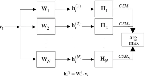
Figure 2: Testing using the supervised NMF classifier (htand vt stand forhtestandvtestrespectively).

During test procedure, each test sound is represented by the feature vector vtest. Afterwards, vtest is projected onto

each class basis matrixWi, yielding:

h(_testi) =W†_i·vtest (8)

For each class, the vectorh(_testi) is compared to each column vector of matrixHiusing the cosine similarity measure. The

vector that maximizes the CSM for the matrix Hi is

calcu-lated as a measure of similarity for this class:

CSM_i= max

j=1,2,...,r_i

_h(i)T testh(

i) j

h_test(i) h(_ji)

(9)

whereh(_ji)represents the j-th column of matrixHi. Finally,

the class label of the recording is determined by the the max-imumCSM_i, i.e.:

l=arg max

i=1,2,...,N{CSMi} (10)

A block diagram of the testing procedure using the super-vised NMF classification method is plotted in Figure 2.

4. EXPERIMENTAL RESULTS

4.1 Dataset

Audio files extracted from the Musical Instrument Samples database collected by the university of Iowa [1] were used. 300 audio files were extracted that belong to 6 different in-strument classes: piano, violin, cello, flute, bassoon, and so-prano saxophone. In detail, 58 piano recordings, 101 violin recordings, 52 cello recordings, 31 saxophone recordings, 29 flute recordings, and 29 bassoon ones were used. The 300 sounds are partitioned into a training set of 210 audio files and a test set of 90 audio files, which is typical for classifica-tion experiments. All recordings are discretized at 44.1 kHz and have a duration of about 20 sec.

4.2 Feature selection

Regarding the first feature set, for each feature described in Table 1, its mean and its variance were computed, resulting in 41 features in total. The feature dimension of the rhythm

patterns of the second set is 1440, which is quite a large value for training classification algorithms.

In order to reduce the feature vector dimension for both sets, a suitable feature subset for classification has to be se-lected. The optimal feature subset should maximize the ratio of the inter-class dispersion over the intra-class dispersion:

J=tr(S−w1Sb) (11)

where tr(·)stands for the trace of a matrix,Swis the

within-class scatter matrix, andS_bis the between-class scatter ma-trix. Because the number of distinct subsets is _(N−N_D!_)!D!, whereDis the desired subset size andNthe feature dimen-sion, the branch-and-bound search strategy is considered for complexity reduction. In this strategy, a tree structure of

(N−D+1)levels is created, where every node corresponds to a subset. The highest level corresponds to the full set, while each node corresponds to aD-dimensional subset at the lowest level. The branch-and-bound algorithm traverses the structure using a depth-first search with backtracking [11].

4.3 Performance Evaluation

Two separate experiments on the various NMF algorithms have been performed by using the two feature sets described in Section 2. Subsets of the feature sets were created using feature selection, in order to find the feature dimension that maximizes the classification performance. For the first set, 6 features were used from the total 41 (mainly the moments of the first two MFCCs). For the second set, 50 features were selected from the total 1440.

NMF Algorithm

Mean

classification

accurac

y

%

Feature Set 1 Feature Set 2

NMF LNMF SNMFλ=0.1 SNMFλ=0.001

[image:5.595.310.542.412.591.2]

70 75 80 85 90 95 100

Figure 3: Mean classification accuracy for NMF algorithms.

[image:6.595.49.287.252.337.2]

classification [9]. In addition, the results using the first set outperform the supervised classifiers based on gaussian mix-ture models (GMM) and continuous hidden Markov models (HMM) also utilized in [9]. Generally, the performance of the classifier diminishes when the second feature set is uti-lized. The main reason is the large feature dimension of the rhythm patterns, which could be diminished by using sta-tistical moments to describe the feature vector. The highest accuracy for the second set is achieved using the SNMF algo-rithm forλ=0.1, being 93.1%. The LNMF is clearly outper-formed by all algorithms, which may be explained due to the locality constraints LNMF imposes when applied to holistic descriptors. The SNMF overall displays better results than the LNMF, but its efficiency depends on the selection of pa-rameterλ (performance is slightly better whenλ = 0.001).

Table 2: Confusion matrix for standard NMF, Feature Set 1.

Instr. Piano Bassoon Cello Flute Sax Violin

Piano 18 0 0 0 0 0

Bassoon 0 9 0 0 0 0

Cello 0 0 16 0 0 0

Flute 1 0 0 8 0 0

Sax 0 0 0 0 9 0

Violin 0 0 0 0 0 29

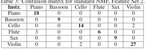
Table 3: Confusion matrix for standard NMF, Feature Set 2.

Instr. Piano Bassoon Cello Flute Sax Violin

Piano 18 0 0 0 0 0

Bassoon 0 9 0 0 0 0

Cello 0 0 14 0 0 2

Flute 3 0 0 6 0 0

Sax 0 0 0 0 9 0

Violin 0 0 2 0 0 27

Additional information about the performance of the standard NMF algorithm using the two sets is shown in Ta-bles 2 and 3 in the form of a confusion matrix. The columns of the confusion matrix correspond to the predicted musical instrument and the rows to the actual one. For the first set, a single misclassification occurs. For the second set, most misclassifications occur for the flute, as well as for the violin and cello.

5. CONCLUSIONS

In this paper, a method of classifying musical instrument recordings by using supervised NMF classifiers using two different feature sets has been presented. The results indicate that the standard NMF algorithm used in conjunction with the first set can perform classification with a high accuracy compared to its variants (LNMF and SNMF).

In the future, NMF techniques will be applied to discrim-inate the whole spectrum of orchestral instruments and will be also used in general sound classification experiments. Fi-nally, statistical moments of the rhythm patterns could be used instead of the feature vector in order to improve clas-sification accuracy.

REFERENCES

[1] Univ. of Iowa Musical Instrument Sample Database, http://theremin.music.uiowa.edu/index.html.

[2] MPEG-7 overview (version 9), ISO/IEC JTC1/SC29/WG11 N5525, March 2003.

[3] H. G. Kim, N. Moreau, and T. Sikora, “Audio classifica-tion based on MPEG-7 spectral basis representaclassifica-tions,”

IEEE Trans. Circuits and Systems for Video Technol-ogy, vol. 14, no. 5, pp. 716-725, May 2004.

[4] D. D. Lee and H. S. Seung, “Algorithms for non-negative matrix factorization,”Adv. in Neural Informa-tion Processing Systems, vol. 13, pp. 556-562, 2001. [5] S. Z. Li, X. Hou, H. Zhang, and Q. Cheng, “Learning

spatially localized, parts-based representation,” in Proc.

IEEE Conf. Computer Vision and Pattern Recognition, pp. 1-6, 2001.

[6] C. Hu, B. Zhang, S. Yan, Q. Yang, J. Yan, Z. Chen, and W. Ma, “Mining ratio rules via principal sparse non-negative matrix factorization,” in Proc.IEEE Int. Conf. Data Mining, 2004.

[7] A. Livshin, and X. Rodet, “The importance of cross database evaluation in musical instrument sound classi-fication: a critical approach,” in Proc.Int. Symp. Music Information Retrieval, October 2003.

[8] A. Wieczorkowska, J. Wroblewski, P. Synak, and D. Slezak, “Application of temporal descriptors to musical instrument sound recognition,”J. Intelligent Informa-tion Systems, vol. 21, no. 1, pp. 71-93, July 2003. [9] E. Benetos, M. Kotti, C. Kotropoulos, J. J. Burred,

G. Eisenberg, M. Haller, and T. Sikora, “Comparison of subspace analysis-based and statistical model-based algorithms for musical instrument classification,”2nd Workshop On Immersive Communication And Broad-cast Systems, October 2005.

[10] D. M. J. Tax, One-Class Classification, PhD thesis, Delft University of Technology, The Netherlands, 2001. [11] F. van der Heijden, R. P. W. Duin, D. de Ridder, and D. M. J. Tax, Classification, Parameter Estimation and State Estimation: An Engineerign Approach using MATLAB. London UK: Wiley, 2004.

[12] A. Rauber and M. Fr¨uhwirth, “Automatically analyz-ing and organizanalyz-ing music archives,” in Proc.European Conf. Research and Advanced Technology for Digital Libraries, Springer Lecture Notes in Computer Sci-ence, Darmstadt, Germany, September 2001.

[13] A. Rauber, E. Pampalk, and D. Merkl, “Using psycho-acoustic models and self-organizing maps to create a hierarchical structuring of music by musical styles,” in Proc.Int. Conf. Music Information Retrieval, pp. 71-80, Paris, France, October 2002.

[14] A. Rauber, E. Pampalk, and D. Merkl, “The SOM-enhanced JukeBox: organization and visualization of music collections based on perceptual models,”J. New Music Research, Vol. 32, No. 2, pp. 193-210, June 2003.

[15] T. Lidy and A. Rauber, “Evaluation of feature extractors and psycho-acoustic transformations for music genre classification,” in Proc. Int. Conf. Music Information Retrieval, pp. 34-41, London, UK, September 2005. [16] E. Zwicker and H. Fastl, “Psychoacoustics - Facts and

[image:6.595.49.290.364.445.2]