Pond: A Robust, scalable, massively parallel computer architecture

(1)

Theses Thesis/Dissertation Collections

5-1-2010

Pond: A Robust, scalable, massively parallel

computer architecture

Adam Spirer

Follow this and additional works at:http://scholarworks.rit.edu/theses

This Thesis is brought to you for free and open access by the Thesis/Dissertation Collections at RIT Scholar Works. It has been accepted for inclusion in Theses by an authorized administrator of RIT Scholar Works. For more information, please [email protected].

Recommended Citation

(2)

Architecture

by

Adam R. Spirer

A Master’s Thesis Submitted

in

Partial Fulfillment of the

Requirements for the Degree of MASTER OF SCIENCE

in

Electrical Engineering

Approved by:

Dr. Dorin Patru, Assistant Professor

Thesis Advisor, Department of Electrical and Microelectronic Engineering

Dr. Eric Peskin, Assistant Professor

Committee Member, Department of Electrical and Microelectronic Engineering

Dr. Daniel Phillips, Associate Professor

Committee Member, Department of Electrical and Microelectronic Engineering

Dr. Sohail Dianat, Professor

Department Head, Department of Electrical and Microelectronic Engineering

DEPARTMENT OF ELECTRICAL AND MICROELECTRONIC ENGINEERING KATE GLEASON COLLEGE OF ENGINEERING

ROCHESTER INSTITUTE OF TECHNOLOGY ROCHESTER, NEW YORK

(3)

Rochester Institute of Technology Kate Gleason College of Engineering

Title:

Pond: A Robust, Scalable, Massively Parallel Computer Architecture

I, Adam R. Spirer, hereby grant permission to the Wallace Memorial Library to repro-duce my thesis in whole or part.

Adam R. Spirer

(4)

Acknowledgments

Thank you to my family and my colleagues for supporting me in this research and the writing of this document, specifically to my advisor Dr. Dorin Patru and my committee

(5)

Abstract

Pond: A Robust, Scalable, Massively Parallel Computer Architecture Adam R. Spirer

Supervising Professor: Dr. Dorin Patru

(6)

List of Tables

2.1 Configuration and data processing fields for an AP . . . 7

2.2 Atomic Processor Instruction Set . . . 9

3.1 Handshake codes for atomic processor communications . . . 13

3.2 Transmit directions for global (G), beamed (B), and entity (E) casts . . . . 14

3.3 Message buffer format for result message. All number represent bits. . . 15

[image:9.612.115.526.182.465.2]

3.4 Message buffer format for coded message types; codes are described in Table 3.5. All numbers represent bits. . . 15

3.5 Message codes and descriptions for non-result message types . . . 17

5.1 Summary of performance metrics, measured in cycles . . . 35

6.1 Variables table generated for data structure for vector addition code . . . 51

6.2 Variables table generated for data structure for vector addition code . . . 53

6.3 Vector addition machine code for function definition elements . . . 55

6.4 Vector addition code machine code for data structure elements . . . 56

6.5 Fibonacci series machine code for function definition elements . . . 58

(10)

List of Figures

2.1 A simple representation of the atomic processor sea. . . 4 2.2 An example sea of APs, populated with functions and data. . . 5

3.1 Message and handshake buffers in an atomic processor. . . 12 3.2 Timeline of handshake process; APxis sending a message to its neighbor,

APy. . . 13 3.3 Propagation of communication casts in the sea. . . 14 3.4 Send and receive layers of communication buffer circuitry. . . 18

4.1 Atomic processor moving around an entity; the dashed line indicates the desired path, and the solid lines represent the redirected path the entity takes. 20 4.2 Timeline of an instruction cycle, including communication broadcasts. . . . 24 4.3 Input/output interface at border of sea. . . 26 4.4 Examples of loop handling in the architecture: program flow for loop

iter-ations created as separate functions, program flow for parallelizable loop iterations executed within a single function, and program flow for sequen-tial loop iterations executed within a single function. . . 28

5.1 Examples of best case 100% parallelizable code, worst case 100% par-allelizable code, best case 100% sequential code, and worst case 100% sequential code. . . 32 5.2 Example multiplication superentity using left-shift algorithm. . . 37 5.3 Example integer division superentity. . . 39 5.4 Example floating point multiplication superentity, including use of integer

multiplication function for operating on significands. . . 41

6.1 Vector addition code as superentity, derived from machine code represen-tation. . . 57 6.2 Fibonacci series code as superentity, derived from machine code

(11)

7.1 Software screen capture of Simulator window with loaded processor sea. . . 67 7.2 Software screen capture of AP Record view. . . 68 7.3 Software screen captures of global cast propagation; consecutive machine

cycles are shown. . . 69

(12)

Chapter 1

Background and Motivation

Parallelism and concurrency are inherent in many computational tasks. Techniques that

ex-ploit instruction and thread level parallelism in traditional von Neumann architectures have

been successfully applied in single processors, as described by Hennessey and Patterson

in [1]. During the past decade researchers and manufacturers have turned to multi-core

processors, which at the present time are limited to just a few cores [2–7]. Scaling up the

techniques used to exploit instruction and thread level parallelism in single core processors

to many core processors is challenging for both hardware and software designers [8–11].

As pointed out by Hennessy and Patterson in [1], multi-core processors are a

combi-nation of computer architecture and communications architecture. Computer networks on

a chip or cluster computing on a chip are adapting the vast knowledge base of designs

and architectures of macro computer networks to the micro scale, [12–24]. Marculescu

et al. in [25] classify outstanding research problems related to networks on chip into 15

categories. Predominant are problems related to communications infrastructure and

com-munications paradigms, as illustrated by [26–52]. Dongarra et al. explore the potential

symbiosis between networks on chip and multicore processors in [53].

Late and post silicon era integrated circuit fabrication technologies will continue to

in-crease the number of components on a chip to billions and trillions. The sheer inin-crease in

number will not translate into an increase in performance unless new parallel and

(13)

et al. in [55]. These new architectures will have to address reliability at the circuit and

system levels because some components will experience premature, transient or permanent

failures, as highlighted by Austinet al.in [56]. Lei Zhanget al.address reliability and fault

tolerance in networks on chip in [57]. Power dissipation will have to be mitigated starting

at the system level. This is already being considered in multicore processors [58, 59], and

in networks on chip [60–65]. Nano architectures attempt to specifically address the

afore-mentioned challenges posed by late and post silicon technologies [66–74].

In this thesis, an architecture is proposed, which can efficiently use a few hundred to

multi-billion cores. Its implementation is cost effective in late and post silicon

technolo-gies, resilient to component failures, massively parallel, and can support a high degree

of concurrency without a radical paradigm shift in programming. The architecture shares

traits with multicore processor architectures, networks on chip, nano architectures,

mas-sively parallel architectures, resilient and fault tolerant architectures, reconfigurable

com-puting, data flow architectures, and neural networks. These similarities and differences will

be discussed after the proposed architecture is presented.

In Chapter 2, the organization of the architecture is covered, followed by the

communi-cations architecture in Chapter 3, operation in Chapter 4, performance evaluation in

Chap-ter 5, programming in ChapChap-ter 6, architectural features and benefits in ChapChap-ter 8, related

(14)

Chapter 2

Architecture

As discussed in Chapter 1, a primary question in developing an effective parallel computing

system is the number of cores. Both extremes have been observed; some architectures

implement a small number of complex cores, while others implement a large number of

simple cores. The proposed architecture takes the latter approach and implements a

fine-grained system with a large number of simple cores.

2.1

Organization

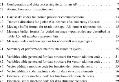
Figure 2.1 shows the top-level layout of processing cores, calledatomic processors(APs)

for this architecture.

As shown, the architecture is composed of a grid-like sea of APs. An AP at a given

time will either act as a program instruction (including associated operands), or a

stor-age element containing one data word. Each AP has all the hardware it needs to

exe-cute any instruction, theoretically allowing for all available instruction-level parallelism to

take place. Programs on the architecture are logically organized into function definitions

(FD) consisting of multiple APs containing instructions, which are called to execute when

needed. At runtime, function definitions are called to execute as function instances (FI)

which are copies of the corresponding function definition, and are capable of operating on

(15)

AP

[i,j] [i,APj+1] AP

[i,j-1] AP

[i-1,j-1] [iAP-1,j] [i-1,APj+1]

AP [i+1,j+1] AP

[i+1,j] AP

[image:15.612.128.492.88.334.2]

[i+1,j-1]

Figure 2.1: A simple representation of the atomic processor sea.

logically-organized groups of APs are collectively calledentities. These entities are capable

of “moving” through the sea of processing elements by way of transferring their individual

instructions and data words (entity elements) to adjacent APs, allowing them to interact

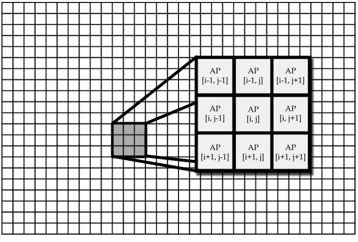
with other entities. Figure 2.2 shows an example of what a populated small processing sea

might look like (actual sea and program/data sizes will be significantly larger to reflect the

application).

Each AP is capable of storing both a function definition element, and a function instance

or data structure element, at the same time. This breaks down the sea into two logical

layers: thedefinition layer(function definitions) and theexecution layer(function instances

and data structures). Composed of common high-level programming constructs—function

definitions, instances, and data structures—execution of programs takes place in much the

same way as in traditional architectures.

Instantiation of the function is equivalent to the function call in high-level programming,

(16)

[image:16.612.129.494.86.386.2]

Function Definition (FD) Function Instance (FI) Data Structure (DS)

Figure 2.2: An example sea of APs, populated with functions and data.

APs, creating a function instance. The function instance can then move and interact with

data structures, which are also present in the execution layer. Interaction between function

instances and data structures is preceded by a move and abut process, in which the function

instance locates the data structure of interest and abuts it, creating a superentityin which

instructions can fetch data as needed.

Each AP is functionally identical and operationally independent. In addition to

stor-ing operands and processstor-ing circuitry, configuration information is stored—information

to identify the entity number, individual entity element number, execution order number

(to indicate when the instruction can execute), and other information generated at compile

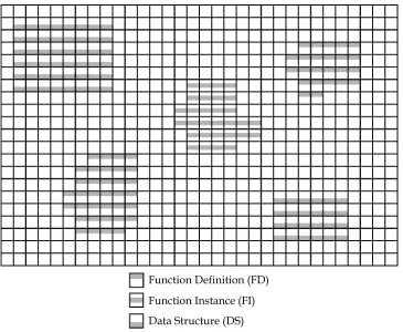
time. Table 2.1 and shows all the independent configuration fields present in a single AP, as

well as operand/data fields. These fields are duplicated for the standby layer (for function

(17)

only exceptions noted are that the entity type field is slightly different between the two

lay-ers, and data operand and some other execution-time values are not present in the standby

layer. Development is currently being done using a sea of 64 K atomic processors, which is

considered to satisfy the needs of an embedded computer system. Field bit widths are also

shown in Table 2.1 for 1 Tera atomic processors, which is considered to satisfy the needs

of a desktop computer system.

The fields presented in Table 2.1 provide space for all necessary data, instruction

oper-ation code, execution conditions, and the informoper-ation necessary to exploit the parallelism

and concurrency discovered at compile time. This also allows for concurrency in

instruc-tions within a function instance, allowing for convergence back to sequential operation if

needed. In addition, all APs are identified physically and logically. In terms of instruction

execution once operands have been loaded (which will arrive via a communications

broad-cast from another AP in the sea; more on this in Chapter 3), each AP is independent and

does not require the resources of any other AP. APs are synchronous blocks, but the entire

sea can be asynchronous, as there is no specific need for neighboring APs to operate

syn-chronously. This eliminates the need for global clock synchronization, a common design

issue in large circuits. While implementing this architecture via a globally asynchronous,

locally synchronous strategy is possible, there are many issues to address in terms of the

asynchronous interfaces among blocks [75–78]. In silicon technologies, fields could be

implemented with SRAM cells similar to the way FPGA configuration bits are held (this

is a topic for future work and is discussed in Chapter 10). Note that the data widths for ID

numbers, execution order, and execution repeat values are defined by the sea size; however,

a 64K sea size is assumed in this presentation.

2.2

Instruction Set

(18)

[image:18.612.96.521.132.678.2]

Table 2.1: Configuration and data processing fields for an AP Name Bits, 64K Bits, 1T Value

Entity Type (Standby) 1 1 0=Unoccupied; 1=FD element

Entity Type (Execution) 2 2 0=Unoccupied; 1=FI element; 2=DS Element Hardware ID 16 40 X-Y physical location of element

Entity ID 16 40 Entity logical ID number Element ID 16 40 Entity element logical ID number

Target Entity ID 16 40 FI: Entity ID of the data structure that the FI entity is associated with

Primary Operand/Data Word (Execu-tion Only)

32 64 FD/FI: Primary operand value; DS: Data word value

Secondary Operand (Execution Only) 32 64 FD/FI: Secondary operand value

Primary Operand ID 16 16 FD/FI: Primary operand ID, corresponds to an as-sociated DS entity or element ID

Secondary Operand ID 16 16 FD/FI: Secondary operand ID, corresponding to associated DS entity ID or element ID

Primary Operand Type 4 4 FD/FI: Primary operand type; for future imple-mentation

Secondary Operand Type 4 14 FD/FI: Secondary operand type; for future imple-mentation

Operation Code 8 8 FD/FI: Instruction/operation code

Execution Conditions 8 8 FD/FI: Status bits (C, N, V, Z, !C, !N, !V, !Z) re-quired for execution of instruction

Status Bits ID 16 40 FD/FI: Element ID whose execution result pro-duces the status bits for this instruction (compared against execution conditions)

Execution Order 16 40 FD/FI: Element execution order number

Prev.-Execution Order 16 40 FD/FI: Execution order number of element(s) that must execute before this element

Result Value (Execution Only) 32 64 FI: Result value of last execution Status Bits (Execution Only) 8 8 FI: Resulting status bits of last execution Execution Count (Execution Only) 16 16 FI: How many times must this FI receive a result

broadcast with a particular execution order num-ber (from a previous instruction) before executing itself?

Execution Count ID 16 40 FI: Associated DS Element ID that holds the exe-cution count value

Message Code (Execution Only) 8 8 FI: Message code for move, abut, and other special communications operations

Total to Store: 338 698

To move FD/FI element: 226 482

(19)

codes. The instruction set has been chosen to include all arithmetic and logic operations.

Each instruction can be conditional or unconditional.

The instruction set qualifies as a reduced instruction set, keeping with the desired goal

to have simple processing elements. This does not limit the overall processor/architecture

in terms of complexity; any complex operation can almost always be implemented as a set

of smaller operations. The given instruction set supports very common RISC instructions

that are capable of compounding to the complex operations that may be required by an

application. That is, multipliers, floating point units, and other traditional function units can

be implemented as entities containing the appropriate sequence of instructions to execute.

Note that these functions will be “soft” in that they will be inherently tailored at compile

time to the application at hand, making them further efficient.

A given function may have multiple RETURN instructions that can be reached, just

as in most functions in high-level languages. However, in this case, multiple RETURN

instructions may be executed in the same path to allow more data to be sent from the called

function back to the calling function. Regarding execution counts, the default behavior is an

execution count of 1, which will be realized if the FI element’s execution count ID matches

its own element ID. That is, as soon as an FI element receives a message that another FI

element with an execution order number that matches its previous-execution order number,

then it will execute. In the case where there are execution conditions, the FI element will

also compare the message’s source element ID to its own status bits ID when considering

the previous-execution order number, only executing if the element ID and status bits ID

values match. All instructions are therefore capable of conditional execution. However, if a

FI element’s status bits ID matches its own element ID, then the execution conditions field

(20)

[image:20.612.105.514.161.644.2]

Table 2.2: Atomic Processor Instruction Set Mnemonic Operation Code Operation

NOP 0x00 No operation.

ADDPS 0x01 Add primary and secondary operands. ADDPC 0x02 Add carry and primary operand.

ADDPSC 0x03 Add primary operand, secondary operand, and carry. SUBPS 0x04 Subtract secondary operand from primary operand. SUBPC 0x05 Subtract carry from primary operand.

SUBPSC 0x06 Subtract secondary operand and carry from primary operand. INC 0x07 Increment primary operand.

DEC 0x08 Decrement primary operand. INV 0x09 Bitwise inversion of primary operand.

AND 0x0A Bitwise AND of primary and secondary operands. OR 0x0B Bitwise OR of primary and secondary operands. XOR 0x0C Bitwise XOR of primary and secondary operands. SETC 0x0D Explicitly set ‘carry’ flag.

SETZ 0x0E Explicitly set ‘zero’ flag. SETN 0x0F Explicitly set ‘negative’ flag. SETV 0x10 Explicitly set ‘overflow’ flag. RSTC 0x11 Explicitly reset ‘carry’ flag. RSTZ 0x12 Explicitly reset ‘zero’ flag. RSTN 0x13 Explicitly reset ‘negative’ flag. RSTV 0x14 Explicitly reset ‘overflow’ flag.

SHL 0x15 Shift left primary operand, pad with zeroes. SHR 0x16 Shift right primary operand, pad with MSB.

SHLC 0x17 Shift left primary operand through carry, pad with zeroes. SHRC 0x18 Shift right primary operand through carry, pad with MSB. CALL 0x19 Function call instruction; requests instantiation of function

def-inition logical ID# in primary operand to process data structure logical ID# in secondary operand. Execution of this instruction completes when the instruction receives a RETURN result from the called function instance.

(21)

2.3

Implementation of Compound Operations

As shown in Section 2.2, each AP supports only a small set of simple integer manipulation

instructions, holding true to the philosophy of processing via a large number of simple

pro-cessing elements. More complex operations such as multiplication and floating point

op-erations are very commonly used in many applications, and a successful high-performance

architecture should implement these functions efficiently. These compound instructions

can be implemented as function definitions that are called when required by other function

(22)

Chapter 3

Communications

The communication architecture driving these processing APs uses nearest-neighbor

com-munication methodology; each AP can communicate directly with its eight adjacent

neigh-bors. In the case of communication with non-adjacent processors, neighboring APs are

capable of acting as conduits for passing messages to other APs in the sea. These

com-munications may take place as broadcasts in all directions to either the entire sea or just a

specific function definition, instance, or data structure (anentity), or a directional broadcast

to a specific AP inside or outside the entity.

3.1

Handshaking

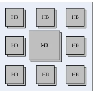
The APs in the sea communicate via a set of eight pairs ofhandshakebuffers (two for each

neighbor; one to send messages and one to receive messages) for handshaking, as well as a

common message buffer for passing messages and data once communication initialization

has been established via the handshaking protocol. Each AP, as well as its eight neighbors,

can write to and read from these buffers. The buffers are shown visually in Figure 3.1.

In addition, a dual message buffer (one to store a message to be sent, and one to load a

received message).

The handshaking algorithm is a three-step process using the handshake buffer. A

(23)

HB MB

HB

HB HB

HB

HB HB

HB

HB HB

HB

HB HB

HB

[image:23.612.232.389.87.240.2]

MB

Figure 3.1: Message and handshake buffers in an atomic processor.

buffer filled in the next cycle. If and only if the handshake buffer is currently set to 0, APx

initiates a request to APyby filling APy’s corresponding handshake buffer with a specific

handshake code. The code specifies the particular type of communication that will take

place. This completes cycle 1 of the handshake. Next, AP y indicates its availability to

receive a message in the message buffer by resetting the handshake buffer back to 0. This

completes cycle 2. Finally, APxloads the contents of its message buffer (the message/data

it wishes to send) into AP y’s message buffer. This completes cycle 3, and the

commu-nication cycle is complete. Naturally, there will be many cases where requests arrive to a

particular AP from multiple neighbors at the same time. The AP will process one request

at a time; the remaining APs will wait for their request to be served-as described in cycle

2, AP yindicates its availability by resetting the appropriate handshake buffer. Until this

occurs, APxwill wait. Priority in communication handling is also implemented; priorities

are based on the handshake code, and certain codes will be accepted before others.

Figure 3.2 shows a timeline representation of a communication cycle in which on

(24)

[image:24.612.102.516.306.655.2]

Figure 3.2: Timeline of handshake process; APxis sending a message to its neighbor, APy.

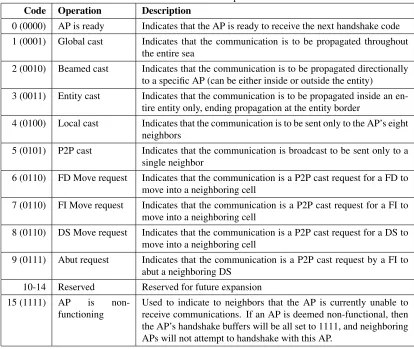
The handshake codes are 4 bits wide, and are shown in Table 3.1.

Table 3.1: Handshake codes for atomic processor communications

Code Operation Description

0 (0000) AP is ready Indicates that the AP is ready to receive the next handshake code 1 (0001) Global cast Indicates that the communication is to be propagated throughout

the entire sea

2 (0010) Beamed cast Indicates that the communication is to be propagated directionally to a specific AP (can be either inside or outside the entity)

3 (0011) Entity cast Indicates that the communication is to be propagated inside an en-tire entity only, ending propagation at the entity border

4 (0100) Local cast Indicates that the communication is to be sent only to the AP’s eight neighbors

5 (0101) P2P cast Indicates that the communication is broadcast to be sent only to a single neighbor

6 (0110) FD Move request Indicates that the communication is a P2P cast request for a FD to move into a neighboring cell

7 (0110) FI Move request Indicates that the communication is a P2P cast request for a FI to move into a neighboring cell

8 (0110) DS Move request Indicates that the communication is a P2P cast request for a DS to move into a neighboring cell

9 (0111) Abut request Indicates that the communication is a P2P cast request by a FI to abut a neighboring DS

10-14 Reserved Reserved for future expansion 15 (1111) AP is

non-functioning

Used to indicate to neighbors that the AP is currently unable to receive communications. If an AP is deemed non-functional, then the AP’s handshake buffers will be all set to 1111, and neighboring APs will not attempt to handshake with this AP.

(25)

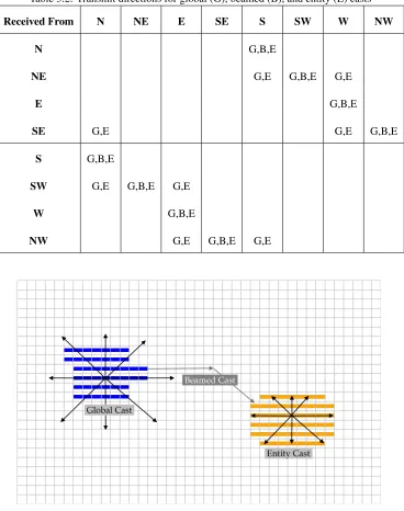
directions for global, entity, and beamed casts. Figure 3.3 shows visual examples of the

[image:25.612.127.495.147.613.2]

casts’ propagations in the sea.

Table 3.2: Transmit directions for global (G), beamed (B), and entity (E) casts

Received From N NE E SE S SW W NW

N G,B,E

NE G,E G,B,E G,E

E G,B,E

SE G,E G,E G,B,E

S G,B,E

SW G,E G,B,E G,E

W G,B,E

NW G,E G,B,E G,E

(26)

3.2

Message Passing

The message buffer contains the actual message to be communicated as well as the

re-quired decoding information such as source and destination identification information and

locations. Table 3.3 and Table 3.4 describe the two different formats of the message that

is transferred through the message buffer. The former is for broadcasting entity cast

re-sults from instruction executions; the latter is used for other non-result communication

messages.

Table 3.3: Message buffer format for result message. All number represent bits.

Sea Size Message Type

Source ID Result Value P/S Operand E. O. Number Status Bits

Reserved Total Bits

64 K 4 16 32 32 16 8 20 128

1 T 4 40 64 64 40 8 44 256

Table 3.4: Message buffer format for coded message types; codes are described in Table 3.5. All numbers represent bits.

Sea Size Message Type

Source ID Dest. ID Inter. ID ID Type: S/D/I

Reserved Total Bits

64 K 4 16 16 16 2/2/2 70 128

1 T 4 40 40 40 2/2/2 126 256

The shaded fields are fields in which the bit width depends on the sea size. As shown,

the result message type has the capability of storing both the execution result value as well

as a primary or secondary operand from the broadcasting element; this allows for future

extension where instructions may change operand values and need to broadcast them to

keep all other copies of that element updated in the entity. In the coded message type, the

ID Type field is broken into S, D, and I fields, corresponding to source, destination, and

intermediate ID numbers with which the message is associated. The source and destination

IDs are the sending and receiving ID numbers, and the intermediate ID number is used for

other entities or elements associated with the message. These numbers can be either entity

(27)

that in both message types, there is reserved space for future extension.

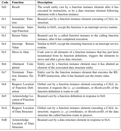
Table 3.5 shows all current message codes utilized by the architecture.

3.3

Send and Receive Layers

One may expect the nature of the communication architecture to present an issue with

message backup. With many messages passing in a single entity, it is conceivable that

collisions in messages could occur, causing stalls and therefore delay in execution, if the

message passing is not handled appropriately. To avoid backup, each AP contains two sets

of handshake buffers and two sets of message buffers; one set is dedicated to receiving

messages and one set is dedicated to sending messages, essentially creating a bi-directional

message passing system that limits the possibility of collisions. Since each AP contains

a dedicated buffer for receiving and sending, an AP can both receive and send a message

at the same time to any neighboring processor. The only time when a message will need

to wait for more than one communication cycle is if it arrives at the same time with

an-other message from anan-other AP. If this does occur, the priority handshaking discussed in

Section 3.1 is capable of handling simultaneous messages through priority settings. There

is a form of communication back-off inherent in this system; in the case of simultaneous

message receipt caused by a number of close entity casts, the priority-based handling of

the receiving AP will naturally “stagger” the casts after the first collision, helping to

pre-vent further collisions. Also, collisions will only occur at the “wave fronts” of the casts.

Once the communication cycle in which collision occurs is completed, there are no further

conflicts.

Figure 3.4 shows the message and handshake buffer connections between two

(28)

[image:28.612.112.510.189.621.2]

Table 3.5: Message codes and descriptions for non-result message types

Code Function Description

0x0 Result The result entity cast by a function instance element after it has executed its instruction, or by a data structure element following abutment with a function instance.

0x1 Instantiate Func-tion

Beamed cast by a function instance element executing a CALL in-struction.

0x2 Instantiate Inter-rupt Function

Similar to 0x01, except the function is an interrupt service routine.

0x3 Return Value Beamed cast by a called function instance to the calling function instance, after it has completed execution.

0x4 Interrupt Return Value

Similar to 0x03, except the returning function is an interrupt service routine.

0x5 Move to Abut Code sent to all elements of a function instance that has just been instantiated from its function definition; triggers the elements to move and abut a given data structure.

0x6 Abutment Com-pleted

Entity cast by a function instance element once it has abutted an element of the associated data structure entity.

0x7 Terminate Func-tion Instance En-tity

Entity cast by the function instance element that executes the RE-TURN instruction, after it has beamed cast the return value.

0x8 Request Location of Function Defi-nition

Global cast by a function instance element executing a CALL in-struction; it requests the (x,y) coordinates, orHardwareID, of the function definition it wants to call.

0x9 Acknowledge Lo-cation of Function Definition

Beamed cast by a function definition in response to 0x8.

0xA Request Location of Data Structure

Global cast by a function instance element executing a CALL in-struction; requests (x,y) coordinates, orHardwareID, of the data structure the called function wants to process.

0xB Acknowledge Location of Data Structure

(29)

[image:29.612.181.436.85.301.2]

Figure 3.4: Send and receive layers of communication buffer circuitry.

Note that according to Figure 3.4, the message buffers (MB) on both layers are

con-nected; in the case where an AP is only propagating a message and not processing it, the

propagating message can be loaded directly into the Send layer, saving a clock cycle and

(30)

Chapter 4

Operation

4.1

Entity Movement

This is a special case of the P2P cast, using a command message broadcast. A move request

is sent to a specific AP by a neighbor when that neighbor (an entity element) wants to move

into that AP’s cell. This would obviously only take place with that AP were empty, i.e.,

it does not contain a function definition element (in the case of the standby layer) or a

function instance or data structure element (in the case of the execution layer). A single

move operation is described in the following steps:

1. In cycle 1, APx(which contains one element of an entity) requests to move into AP

yby setting APy’s handshake buffer to code 6.

2. In cycle 2, APywill reset its handshake buffer back to 0. In addition, APywill fill AP

x’s message buffer with a specific message indicating either an affirmative or negative

response to the move request.

3. In cycle 3, if the move request was answered affirmatively, then AP x will transfer

into AP y’s cell. If the response was negative, then AP xwill need to use the same

communication process on its other neighbors to attempt an alternative path to move.

The algorithmic development of the movement algorithm to be implemented in

(31)

together referred to as acommunication cycle. The transfer of AP contents from one cell to

another is accomplished via either a parallel interface or the message buffer. In the former

case, each field as described in Table 2.1 is multiplexed to those of its neighbors,

allow-ing the simultaneous transfer to take place. In the latter case, two cycles would be used

for transmitting required fields over the limited message buffer size. In either case, for

simplicity, we will refer to a single move operation as one communication cycle.

Naturally, an AP in the sea may encounter other APs from other entities along its path

that impede its movement along that usually direct path. In this case, the AP will attempt

to move in an alternative direction into an available cell, and then again try to move in the

[image:31.612.142.478.319.531.2]

target direction in the next cycle. Consider the example shown in Figure 4.1.

Figure 4.1: Atomic processor moving around an entity; the dashed line indicates the desired path, and the solid lines represent the redirected path the entity takes.

As shown in Figure 4.1, an entity element that must redirect its path around another

entity will do the following:

1. Element moves one step in either a counterclockwise (CCW) orclockwise (CW)

di-rection as a redirected path (for example, a target southeast movement will redirect to

(32)

2. Element repeats step 1, continuing its attempt to move around the entity in a CCW or

CW direction.

3. Element eventually clears the entity and is able to move unobstructed towards its

target.

Note that there is some extra delay when an element must move around an entity. Since

the initial move request is rejected, two extra machine cycles occur for the element to move

into its next cell, making a communication cycle a total of five machine cycles instead of

the usual three machine cycles.

4.2

Entity Abutment

This is also a special case of the P2P cast, using a command message broadcast. This

communication is made to a neighboring processor when a function instance wants to

as-sociate with a data structure. Once the function instance hits a data structure, it initiates

an abutment request to obtain the data structure’s logical ID number at which time it can

then decide if it is the correct data structure to process (in the case that it is not, the APs

abort the request and attempt to move around the data structure via the method described

in Section 4.1). Abutment is described in the following steps:

1. In cycle 1, APx(which is an element of a FI) requests identification information from

the APy(which is an element of a DS) in order to determine if it is the correct DS to

abut, by setting APy’s handshake buffer to code 6.

2. In cycle 2, AP y will fill APx’s message buffer with its identification information,

and also sets its handshake buffer back to 0 to indicate the request has been served.

3. In cycle 3, AP x will respond by setting AP y’s handshake buffer to 6, and fill its

(33)

contain the other’s identification information, an abutment will occur if the

identifi-cation information is correct, i.e., that particular FI was looking for that particular

DS.

Like the movement algorithm described in Section 4.1, simulation- or

implementation-level algorithms for abutment are in current development. Once abutment completes, the

FI element(s) that abutted send out a coded message indicating abutment has completed,

which is entity cast to the entiresuperentity. Note that multiple command messages may be

sent. Following receipt of this broadcast, every AP in the data structure (DS) portion of the

superentity will broadcast a result broadcast via an entity cast to distribute its current data

word value. This allows instructions to be preloaded with the current state of its operands.

Previous instructions that modify any of these operands will entity cast the updated data

to the appropriate data structure element as well as any instruction in the sea that requires

the use of that particular data storage element. This means that following the initial data

structure broadcast after abutment, all instructions in the function instance (FI) constantly

have updated copies of their data operands, with no need for explicit “memory access” type

procedures.

4.3

Instruction Execution

The execution of an instruction in an AP may be compared to the familiar

fetch-execute-writeback procedure, but note that each of these steps is not exactly as in typical

architec-tures as there is no specific defined memory interface for programs or data. More

specifi-cally, the three steps are most often the following:

1. The needed data operands have been loaded into the AP containing an instruction

(via an earlier result broadcast), and the AP has just received a resultentity cast from

(34)

previous-execution order number. The conclusion of this step means that the

instruc-tion has all the informainstruc-tion it needs to execute and is capable of executing based on

the compile-time discovered parallelism.

2. The instruction is executed locally on the AP with its stored data operands. This may

take one or more machine cycles to execute, but as these are simpleatomicoperations,

they will likely not take any longer than a few clock cycles to complete. Note that the

AP can continue to propagateentity castsandglobal castsbecause the communication

circuitry is independent of the execution circuitry. If a broadcast is received during

execution that mandates that the current execution halt (most likely via aglobal cast;

consider interrupts, discussed in Section 4.7), this is the only case where execution

will be affected by communication activity. The conclusion of this step means that

the instruction execution has completed.

3. The AP sends out a resultentity castaddressed to the data structure element ID

num-ber that should contain the result of the instruction execution. This broadcast will

signal the data structure element as well as any instruction that contains this element

as a data operand (i.e., the data structure element ID number matches the primary or

secondary operand ID numbers). The conclusion of this step means that the result of

the instruction execution has been cast to all locations requiring the data.

Figure 4.2 shows a timeline representation of an entire instruction cycle, including

exe-cution as well as related communication broadcasts.

All instructions defined in Table 2.2 follow this process, with the exception of the CALL

and RETURN instructions, which are described further in Section 4.4. These instructions

utilize the data operands to indicate addresses of data structure and calling/called functions

(35)

Figure 4.2: Timeline of an instruction cycle, including communication broadcasts.

4.4

Function Calls

A function call involves three entities: the calling function, the called function, and the

associated data structure that contains the arguments for the called function. The steps for

this process can be broken into the following, saying functionAcalls functionBto process

data structureC:

1. FunctionA’s CALL instruction (see Table 2.2) will request the (x, y) coordinate

lo-cation of the target/called functionB via aglobal castmessage.

2. FunctionBresponds back to that CALL instruction with the coordinates, via a beamed

cast directed at the (x,y) coordinates of the CALL instruction.

3. FunctionA’s CALL instruction sends a command message beamed cast to function

B indicating it should instantiate and process data structure C, indicating the data

structure’s (x,y) coordinates in the sea.

4. Function definitionB receives the message and instantiates each of its elements into

the execution layer.

5. Function instance B moves to the location of data structure C and initiates an abut

request.

(36)

the rest of the superentity (data structure and abutted function instance) indicating

their element ID numbers and data word values.

7. Once execution of the function completes (that is, a RETURN instruction is ready

to execute), the RETURN instruction sends a beamed message back to the calling

function instance indicating the return value of the called function.

8. The RETURN instruction sends out an entity cast message to its entity indicating that

the function has completed execution and elements should terminate (disappear from

the sea). Meanwhile, function A’s CALL instruction entity casts the return value it

received from the previous step to the rest of its entity.

The actual execution of a function instance always begins with the “first” instruction,

which is specified by the following two conditions:

1. The previous-execution order number is 0

2. The execution order number is 1

Execution conditions are also ignored for the first-time execution of the first instruction;

subsequent executions however will consider the execution conditions as usually expected.

During the entire function call process, the CALL instruction will not move from its

current location, as it relies on beamed cast communications from the called function and

this is location-sensitive. The called function definition also will not move between steps 1

and 2, as this is also a location-sensitive communication process. If a function is to be

in-stantiated multiple times for parallel execution (on different data structures), then multiple

CALL instructions will be used, using the secondary operand to specify the different data

structure entity IDs to use.

Note that “functions” in the sea may or may not be equivalent to the functions or

meth-ods defined in the high-level source code. This is to be decided by the compiler. For simple

(37)

program. For more complex programs with many large functions, the compiler will break

large functions into smaller blocks that share common data or parallelism.

4.5

Input/Output

Input and output points can be defined at the sea’s periphery, using a border AP to load data

into the sea, as shown in Figure 4.3.

U A RT , G PI O , e tc . HB HB Message Passing

[image:37.612.112.495.251.479.2]

MB MB

I/

O

In

te

rf

ac

e

I/ O P or t

Figure 4.3: Input/output interface at border of sea.

Any number of the input/output interfaces as presented in Figure 4.3 can be used along

the border of the sea, allowing for as many I/O pins on a chip as needed for a target

applica-tion. Interfaces can be serial or parallel, and are limited only by the bandwidth requirements

of the given protocol and technology.

To communicate with outside elements, interfaces on each output port can be used to

(38)

4.6

Loops

Loops can be generated in two ways, depending on the complexity of the loop. If a loop

containing only a few sequential operations is needed, then the final instruction in an

it-eration of the loop is used to broadcast the appropriate earlier execution order number,

allowing previously-executed instructions to execute again. Using the execution conditions

to look for a particular condition, the number of executions is defined. This is similar to

current handling of loops in sequential computers, and is the most common way of

imple-menting a loop in assembly programming. For more complex loops that contain a larger

number of instructions that present possible concurrency, a function definition is created

for the loop contents, and the loop can be called multiple times using multiple CALL

in-structions.

The handling of loops depends heavily on decisions made by the compiler related to

discovery of parallelism, discussed more in Section 6.2.3. There are many cases where loop

iterations can be parallelized completely, especially in vector and matrix operations; these

loops can be built as a function definition and instantiated multiple times at runtime. Loops

can also be implemented as a subset of instructions within a larger function that repeat

execution; this occurs by using the execution order number to trigger earlier instructions to

execute again if a given condition for running subsequent loop iterations is true. Of course,

instruction-level parallelism within a single loop iteration is always possible via the use of

the execution order number (i.e., instructions that can execute concurrently have the same

execution order number), as it is for any instruction in a loop iteration or not. Figure 4.4

(39)

[image:39.612.111.510.89.325.2]

(a) (b) (c)

Figure 4.4: Examples of loop handling in the architecture: program flow for loop iterations created as separate functions, program flow for parallelizable loop iterations executed within a single function, and program flow for sequential loop iterations executed within a single function.

4.7

Exception Handling

Exception can be handled at the input/output ports through the use of the global cast,

uti-lizing the command message broadcast format, similarly to the way a function call is

per-formed. The exception will propagate through the entire sea, eventually reaching all APs.

Since global casts are of highest priority, the propagation will not be halted by any other

communications within entities, allowing the exception to be processed as soon as it reaches

the exception handling function (routine). Below is a non-exhaustive list of exceptions, as

described in [1], that will have to be considered:

• Hardware device interrupts

• Breakpoints/debug interrupts

• Arithmetic overflow

(40)

• Undefined/unimplemented instruction

• Hardware malfunctions

• Power failure (requires halting of each AP operation once the exception is received)

Only the power failure will affect all morphological entities and all atomic processors

in the sea. All other exceptions will affect the entities to which they relate. Exceptions

will not stop other communications currently propagating in the sea once the “wave front”

of the exception has passed (as the exception will have higher priority than other

com-munications, those other communications will have to wait for a communication cycle to

allow the interrupt to pass through). That is, while an exception is propagating in the sea,

all other currently propagating communications—result entity cast messages, mostly—will

complete their traveling to their destination, and will update their data structure elements

and data operand values. This is to maintain consistency in data throughout the sea, as the

(41)

Chapter 5

Performance Evaluation

5.1

Machine Cycle

A machine cycleis assumed to be the standard local instruction cycle on an AP. This

in-cludes just the time for execution of the instruction as well as decoding of the message

buffer (analogous to instruction fetch) and encoding of the result message (analogous to

writeback)—in other words, a fullexecution cycle. In addition, a machine cycle is assumed

to encompass the amount of time for handshaking and message buffer transfer (also known

as a fullcommunication cycle.

5.2

Minimum and Maximum Execution Times

The total execution time of a called function, from the moment the calling function

in-stance sends out the CALL message, and until it receives the return message and/or data

structure, depends on the duration of the following events: call to instantiate, instantiate,

move to abut, abut, effective execution, and RETURN. In turn, the duration of all these

events depends on the sizes of the called function instance and its associated data structure,

and except for the effective execution time, on the relative location of the calling function

instance and the called function definition, and the relative location of the called function

(42)

therefore known, the times to call, to instantiate, to move, to abut and finally to return, are

a function of the instantaneous computational context. Therefore, their exact values are

best evaluated using a cycle accurate functional simulator, which is discussed in Chapter 7.

However, the effective execution time can be analytically calculated for a few particular

cases. To demonstrate these effective times, some example patterns of execution are shown

(43)

[image:43.612.112.500.88.560.2]

Figure 5.1: Examples of best case 100% parallelizable code, worst case 100% parallelizable code, best case 100% sequential code, and worst case 100% sequential code.

We consider an entity with a square shape and n atomic processors on a side. If the

code is 100% parallelizable, then all elements execute concurrently, except for the one that

(44)

minimum effective execution time is n−₂1+ 1cycles, where the1accounts for the execution

cycle of the return, and n−₂1 for the necessary communication cycles between the elements

at the periphery and the center of the entity, as shown in Figure 5.1(a). Alternatively, if

the element that executes the RETURN element is located at the periphery, the maximum

effective execution time is equal to(n−1)+1, where the 1 accounts for the execution cycle

of the return, and n− 1for the necessary communication cycles between the RETURN

element and the element diagonally opposite from it, as shown in Figure 5.1(b). The total

number of instructions being n2, the minimum CPI or minimum cycles per instruction is

equal to n₂+1_n2, or approximately 1

2n. Similarly, the maximum CPI or maximum cycles per

instruction is equal to _n1. An alternative metric is the IPC, or instructions per cycle, which

is the inverse of the CPI and thus equal to2nandn, respectively.

If the code is 100% sequential or non-parallelizable all elements execute in sequence,

i.e. no two elements execute concurrently. Then, the minimum effective execution time is

equal to 2n2_{, as shown in Figure 5.1(c). This is achieved when the elements executing in}

sequence are always adjacent, i.e. each instruction cycle is equal to the shortest instruction

cycle. The minimum CPI, or minimum cycles per instruction is2, and the maximum IPC,

or the number of instructions per cycle is 1₂.

For the 100% sequential or non-parallelizable code, the worst-case condition is when

each two elements that execute in sequence are located farthest apart, as shown in

Fig-ure 5.1(d) for an8×8sized entity. For convenience, letnbe even andm= n₂. The number

of elements that are located k atomic processors from the center is equal to 4(2k −1),

and their instruction cycle is 2k cycles long, including the execution cycle. Thus the total

execution time of all this elements is4(2k−1)(2k). Notice that moving diagonally,

(45)

4m2_{, the maximum effective execution time is indicated in (5.1).}

TEffExec =

m

X

k=1

4(2k)(2k−1)

= 8 m

X

k=1

k(2k−1)

= 8 m

X

k=1

k2−

m X k=1 k ! = 8

2m(m+ 1)(2m+ 1)

6 −

m(m+ 1) 2

= 4m(m+ 1)(4m−1) 3

= 16 3 m

3 _{+ 4}_m2₋ 4

3

= 2

3n

3₊_n2₋ n

3

≈ 2

3n

3₊_n2

(5.1)

The CPI is indicated in (5.2).

CPI = TEffExec 4m2

= 4

3m+ 1− 1 3m

≈ 4

3m+ 1

= 2

3n+ 1 (5.2)

The performance metrics discussed so far are summarized in Table 5.1. The very good

results for the 100% parallelizable code meet expectations, because of the massively

par-allel character of the architecture. The results for the 100% sequential code with optimal

placement are good. Considered in isolation, the results for the 100% sequential code

with worst placement are at best satisfactorily. However, all these results capture only the

(46)

context of the sea of atomic processors. Intrinsically, the architecture allows thread or

func-tional level parallelism to be fully exploited. This will compensate and further enhance the

overall performance of the architecture. Thread and functional level parallelism can only

be considered in a specific computational context, and are therefore best evaluated using a

cycle accurate functional simulator, which is discussed in Chapter 7.

Table 5.1: Summary of performance metrics, measured in cycles

Performance Metric 100% Parallelizable Code 100% Sequential Code

Minimum Effective Execution Time n+1₂ 2n2

Maximum Effective Execution Time n 2₃n3+n2

Minimum CPI n_n+12 to 1

2n 2

Maximum CPI _n1 2₃n+ 1

5.3

Results

5.3.1 Integer Multiplication

To showcase the implementation of a compound operation, we consider multiplication.

APs do not have dedicated multipliers; multiplication can be done instead by using a

left-shift algorithm. For example, multiplying two numbersxandy, yielding resultz:

1. Initialize a counter to the data word width, or 32 bits for this case.

2. Decrement the counter by 1. If counter value is negative, multiplication is complete.

Else, continue to step 3.

3. If LSB ofxis 1, then addytoz(else, do nothing).

4. Shiftxright by 1 bit, and shiftyleft by 1 bit. Repeat steps 2 through 4.

Figure 5.2 shows an example integer multiplication superentity incorporating the

algo-rithm described above. The following abbreviations may be used for the element fields:

(47)

• POp: Primary operand

• SOp: Secondary operand

• Cond: Execution conditions

• SBID: Status bits ID

• Count: Execution count

• EO: Execution order number

(48)

[image:48.612.103.519.102.543.2]

Figure 5.2: Example multiplication superentity using left-shift algorithm.

To demonstrate cycle-by-cycle operation, each cycle is enumerated below by execution

order number, indication the behavior of APs in each cycle.

1. Step 1: In cycle 1, execution starts with element ID 8, which bitwise ANDs x with

(49)

set to 1. Else, it is reset to 0.

2. Step 2: In cycle 2, if the Z flag is reset to 0, thenyis added toz. At the same time,x

is shifted right andyis shifted left. Else if the Z flag is set to 1, then do nothing. In

either case, the counter is decremented.

3. In cycle 3, if the counter is not zero and not negative, then execution continues again

with step 1. Else, if the counter is zero or negative, then the RETURN element

exe-cutes and the multiplication is complete.

The multiplication algorithm takes the same number of cycles to execute, regardless of

the operand values. The algorithm is effectively two execution steps (enumerated steps 1

and 2 as indicated in the algorithm description in Section 5.3.1) repeated for each bit, in

addition to the return step (enumerated step 3).

5.3.2 Integer Division

To showcase the implementation of another compound operation, we consider integer

divi-sion. APs do not have dedicated dividers; division is instead done using a shift-and-subtract

algorithm. For example, dividing a numbern(numerator) byd(denominator), yielding

re-sult quotientqand remainderr:

1. Initializer=n.

2. Subtractdfromr.

3. If r ≥ 0, then add 1 to q and repeat steps 2-3. Else, add d to r, and division is

complete.

Figure 5.3 shows an example integer division superentity incorporating the algorithm

(50)

[image:50.612.100.518.99.356.2]

Figure 5.3: Example integer division superentity.

To demonstrate cycle-by-cycle operation, each cycle is enumerated below by execution

order number, indication the behavior of APs in each cycle.

1. Step 1: In cycle 1, execution starts with element ID 1, which adds 0 tonand stores in

r(that is,ris assigned ton).

2. Step 2: In cycle 2,dis subtracted fromr. If the result is negative, then the N bit is set

to 1. Else, the N bit is reset to 0.

3. Step 3: In cycle 3, if the N bit it set to 1, then d is added back to r. Else, q is

incremented.

4. In cycle 4, if the N bit was set to 1, then the RETURN element executes and the

(51)

The division algorithm takes a varying number of cycles to execute, as the number of

iterations is dependent on the size of the operands. That is, the number of subtractions

of the divisor from the dividend is the number of iterations the division algorithm must

perform. The more iterations, the longer the execution time.

5.3.3 Floating Point Operations

Floating point arithmetic, multiplication, and other operations are accomplished through

the implementation of special function definitions dedicated to unpacking, processing, and

repacking these numbers when the program needs it. As long as there are APs available

in the sea, as many floating point functions can be instantiated as needed. There are

effec-tively no structural dependencies in providing this functionality, as there are commonly in

processors that use a (usually) limited number of dedicated floating point units, whose use

must be scheduled.

Consider the floating point multiplication algorithm in Equation 5.3.

sp×2ep =s1×2e1 ×s2×2e2 (5.3)

The significand is indicated bysand the exponent bye for an unpacked floating point

number. Figure 5.4 shows an example floating point multiplication superentity, which

con-sists of a multiply operation on the significands (via a function call to the multiplication

(52)

[image:52.612.166.457.98.349.2]

Figure 5.4: Example floating point multiplication superentity, including use of integer multiplication function for operating on significands.

1. Step 1: In cycle 1, execution begins with element ID 2, wheree1 ande2 are added.

2. Step 2: Next,s1 ands2 are multiplied by a call to an integer multiplication function.

Floating point multiplication is now complete.

Note that given the latency required for the CALL operation to implement

multipli-cation, the multiplication function can simply be placed in the function along with the

additional instructions and data required for floating point. The only trade-off is that the

superentity is larger (corresponding to higher communication latency, but this is likely

much lower than the latency associated with a function call).

Consider for completeness the floating point addition algorithm in Equation 5.4.

s×2e =s1+ s2 se1−e2

(53)

This assumes e1 > e2. To compute the significand and exponent of a floating point

addition, a division is required of s2 which can be done via a progressive right shift of

e1−e2times. Following this shift, the result is added tos1and this is the sum’s significand.

(54)

Chapter 6

Programming and Compilation

6.1

Principles

A compiler for this architecture incorporates discovery of parallelism at the high-level (C

programs, for example), followed by assembly into a data stream that will then be

down-loaded to the device, loading the APs with instructions and data. Each instruction and data

element is assigned unique identification information which is used to implement the

par-allelism that is discovered in the compilation process—that is, which specific instructions

can execute in parallel (and which cannot), and which higher-level logical functions can

execute in parallel (and which cannot). What follows the integration of this parallelism is

a program flow unimpeded by resource dependencies or memory access bottlenecks. If a

function has the parameters it needs to execute, it will execute. If an instruction within a

function has the operands it needs to execute, it will execute.

There are a number of steps that must be taken to first discover parallelism in

conven-tional code, and then to determine an appropriate level of implementation of that parallelism

in a given architecture. This architecture is designed to inherently support high-level

pro-gramming concepts (function calls, structured data, iterative processes,etc.) and to resolve

(55)

6.2

Code Conversion Steps

Traditional compilation involves the use of several intermediate representations of the code

before translation to machine code. Usually these representations resolve memory access

routines explicitly, which makes sense in traditional Von Neumann architectures where

memory read/write operations are explicit instructions. In our architecture, memory

op-erations are implicit operations, taking place during execution, but not defined at the

in-struction level. As such, a new representation must be developed that does not explicitly

define memory operations and focuses on the high-level programming concepts that the

architecture supports.

The C programming language can be used as a basis for these developments.

Compila-tion can be broken into the following steps:

1. Parse the code into a clean high-level format.

2. Identify data structures and their elements,i.e., constants and variables; identify

func-tion blocks and instrucfunc-tions within each funcfunc-tion, including funcfunc-tion calls.

3. Discover instruction-level parallelism within functions, including function calls.

4. Generate programming information for each AP based on preceding steps.

6.2.1 Parsing and CIL Representation

The first step in compilation is to parse the input code. C Intermediate Language (CIL) [79]

is an intermediate representation of C that parses and rewrites the code using simple

con-trol structures (only if/else andwhile control structures) while preserving function

definitions, providing explicit variable scope by putting functions further into code blocks,

and also extracting library functions from headers that may be present. Call graphs for

functions may also be generated to indicate dependencies among functions. This cleaner

(56)

which groups of variables should be built into data structures, and where to split up code

into functions.

Giving CIL the source code of a C program we want to convert, the following command

is run:

cilly --save-temps --docallgraph --domakeCFG --dooneRet

--noPrintLn --noInsertImplicitCasts --printCilAsIs --noWrap

source.c > source.c.cg.txt,

wheresource.cis the source C file. [79] Consider the following simple vector addition

code:

int main() {

int vector1[8] = {1, 2, 3, 4, 5, 6, 7, 8};

int vector2[8] = {5, 9, 1, 45, 13, 52, 9, 23};

int i;

for(i=0; i<8; i++) {

vector1[i] = vector1[i] + vector2[i];

}

return 0;

}

CIL will parse this code into the following:

/* Generated by CIL v. 1.3.6 */ /* print_CIL_Input is true */

int main(void)

{ int vector1[8] ;

int vector2[8] ;

int i ;

int __retres4 ;

(57)

vector1[0] = 1;

vector1[1] = 2;

vector1[2] = 3;

vector1[3] = 4;

vector1[4] = 5;

vector1[5] = 6;

vector1[6] = 7;

vector1[7] = 8;

vector2[0] = 5;

vector2[1] = 9;

vector2[2] = 1;

vector2[3] = 45;

vector2[4] = 13;

vector2[5] = 52;

vector2[6] = 9;

vector2[7] = 23;

i = 0;

{

while (1) {

while_0_continue: /* CIL Label */ ; if (i < 8) {

} else {

goto while_0_break;

}

vector1[i] += vector2[i];

i += 1;

}

while_0_break: /* CIL Label */ ; }

__retres4 = 0;

return (__retres4);

}

(58)

while loop structure with continue andbreak labels. In addition, the function

re-turn value is given an explicit variable, compared to the direct constant assignment in the

original code. Both of these results provide a secure basis for generating data structures

and instruction flow for building function definitions.

Consider another example, where we compute the first 12 elements of the Fibonacci

series:

int fibonacci() {

int i;

int a, b;

int c[10] = {0, 0, 0, 0, 0, 0, 0, 0, 0, 0};

a = 0;

b = 1;

for(i=0; i<10; i++) {

c[i] = a + b;

a = b;

b = c[i];

}

return 0;

}

CIL parses the code into the following:

/* Generated by CIL v. 1.3.7 */ /* print_CIL_Input is true */

int fibonacci(void)

{ int i ;

int a ;

int b ;

int c[10] ;

(59)

{

c[0] = 0;

c[1] = 0;

c[2] = 0;

c[3] = 0;

c[4] = 0;

c[5] = 0;

c[6] = 0;

c[7] = 0;

c[8] = 0;

c[9] = 0;

a = 0;

b = 1;

i = 0;

while (i < 10) {

c[i] = a + b;

a = b;

b = c[i];

i ++;

}

__retres5 = 0;

return (__retres5);

}

6.2.2 Semantics Processing

Once the code has been parsed into CIL format, it can be further processed to identify

functions and data structures.

Function definitions indicated in the original code are first given an identification

num-ber. Each variable within each function is also identified, forming a data structure

as-sociated with the function. In addition, multi-instruction loops within functions may be

(60)

(more in Section 6.2.3). In intermediate representation of this step consists of a list of

in-dividual functions and their code, each function supported by a table of variables, logical

identification numbers, and initialization values. The table of variables is a representation

of the data structure that is associated with its corresponding function. Functions and data

structures themselves are also logically identified, allowing cross-referencing for function

calls, as well as allowing for multiple functions to operate on the same data struc

Pond: A Robust, scalable, massively parallel computer architecture