Reliability analysis and optimisation of subsea compression system facing operational covariate stresses

Reliability Analysis and Optimisation of Subsea Compression System facing Operational Covariate Stresses.

Ikenna Anthony Okaro and Longbin Tao*

School of Marine Science and Technology, Newcastle University, Newcastle upon Tyne, NE1

7RU, England, United Kingdom

Keywords: Subsea process system, Subsea control system, Subsea Power System, Reliability analysis, Weibull Analysis, Risk analysis, Human and Operational factors,

Abstract

This paper proposes an enhanced Weibull-Corrosion Covariate model for reliability assessment of a system facing operational stresses. The newly developed model is applied to a Subsea Gas Compression System planned for offshore West Africa to predict its reliability index. System technical failure was modelled by developing a Weibull failure model incorporating a physically tested corrosion profile as stress in order to quantify the survival rate of the system under additional operational covariates including marine pH, temperature and pressure. Using Reliability Block Diagrams and enhanced Fusell-Vesely formulations, the whole system was systematically decomposed to sub-systems to analyse the criticality of each component and optimize them. Human reliability was addressed using an enhanced barrier weighting method. A rapid degradation curve is obtained on a subsea system relative to the base case subjected to a time-dependent corrosion stress factor. It reveals that subsea system components failed faster than their Mean time to failure specifications from Offshore Reliability Database as a result of cumulative marine stresses exertion. The case study demonstrated that the reliability of a subsea system can be systematically optimized by modelling the system under higher technical and organizational stresses, prioritizing the critical sub-systems and making befitting provisions for redundancy and tolerances.

1.0 Introduction

The huge loss and sanctions experienced during the 2010 Macondo oil spill due to the failure of Subsea Blow-out Preventer, the 2011 Bonga incident and a host of recent offshore failures has sparked accelerated efforts towards improvement of reliability, risk management and asset integrity of subsea systems [1][2] [3].

An investigation conducted by the UK Health and Safety Executive [4] indicated that nearly 80% of risk posed to offshore workers emanate from process related failures. These failures which often cause accidents, downtimes and serious economic losses emanate from the complex interaction between human and technical factors which cause approximately 70% and 30% of offshore incidents respectively [5].

deployed to the marine environment are exposed to additional stresses brought by dynamic influencing factors of the sea [6][7]. This justifies any study which seeks to understand the equipment failure behaviour in subsea conditions to ensure maximum uptime. The highly specialized subsea sector is not exactly known for standardized asset life cycle reliability procedures [8] because there seems to be is a lope-sided focus on the technical reliability qualification at manufacturing stages of subsea modules by several scholars; whilst appearing to neglect lifecycle asset reliability especially during the operational stages where the intertwine between human, equipment, environment is more pronounced [9].

Although, risks and failure cannot be completely eradicated from any system, they certainly can be controlled through enhanced reliability strategies throughout the lifecycle of the project. As the world’s first subsea compression system - a joint industry project is currently underway at the Asgard field offshore Norway and planned to commence operations in 2015 [10] [11], major concerns raised by stakeholders bother on reliability, corrosion and production assurance due to past experiences and losses encountered.

This study presents an enhancement to a concept known as Accelerated Life Testing (ALT); an analysis procedure whereby basic system failure data is subjected to a high level of operational stress (covariate) and used to forecast the behaviour of a system [12]. The new approach which adopts a two-prong methodology for both technical and human reliability analysis consists of further development of the works of [13]-[16], where remarkable contributions were made on Weibull-based covariate relationships for technical reliability analysis and human factor analysis respectively.

under normal deep water production operations, water is always present. When CO2 dissolves in water, carbonic acid (H2CO3) is formed which significantly increases the corrosion rate of carbon steels and other materials. The mechanisms of CO2 corrosion under supercritical conditions do not change compared to those identified at lower partial pressure [18].

The behaviour of a subsea system is better understood from a system reliability viewpoint [19] which may connote a reliability study on equipment availability times, an asset integrity assessment, a hazard and operability (HAZOP) study dealing with operability of a system or even a profitability analysis in terms of production capacity and revenue appraisal. In other contexts, it could imply Net Present Value (NPV) of a project, economic and management measures.

At the forefront of reliability analysis techniques is Monte Carlo’s simulation which has been widely used over decades to quantitatively capture the realistic multi-state dynamics and stochastic behaviour of components and systems in reasonable computing times [20].

Lund, [21], developed a statistics-based dynamic model for analysing offshore petroleum projects considering a number of uncertainty factors. The model incorporates several types of flexibility such as drilling options, uncertainties and capacity expansion uncertainties. A case study was carried out using the model and it shows that flexibility in capacity improves a project’s economic value especially when there are many uncertainties surrounding the offshore reservoir. Unfortunately, considerations for human error estimation were not considered in the proposition.

risk analysis by coupling laboratory-derived probabilistic nucleation model with existing deterministic calculations for hydrate growth.

The works of Lin, [24] and Lin [25] suggested flexibility models for deep water oil field systems which were simulated using Monte Carlo’s model to determine the value of specified flexibilities under the uncertainty conditions of reservoir and production capacity [24] [25]. The models did not address the severity of influence on CAPEX and OPEX contrary to Lee et al [26] wherein a design procedure for offshore installations Life cycle Cost Analysis under various environmental load stresses was presented.

System failure data is usually gathered from historical performance archives, but in practice, these data are insufficient and are not always available to reflect the real operational conditions of its purposed domain [27].

In further attempts to account for these operational life conditions, a number of numerical models consisting of life-covariate relationship such as the Arrhenius model, Proportional Hazard model (PHM), Eyring model Extended Hazard Regression, Inverse Power Law had been seen to provide acceptable results [12]. Reliability analysis had been carried out using experimentally or field-sourced sourced failure data and applying predictive models in order to extrapolate results of system reliability beyond the given data range [28]-[35]. For example, in PHM, the operational conditions are considered to be a covariate such that the reliability of the system is a product of time and covariates. The covariate acts multiplicatively on the threshold hazard rate by some constant [14].

The major limitation of life covariate models such as PHM is that they usually has many assumptions which are not applicable in many real world cases. It can only be applied to time-independent covariates; notwithstanding, it is still the most frequently used due to its simplicity and commercial application [15].

the need for representation of stochastic variations related to lifetimes and restoration times using probability distributions while AP1 17N RP provided a structured approach which organisations can adopt for management of uncertainty throughout project lifecycle [36]. Modelling complications are encountered when process variables such as temperatures, mass

flows, pressures, affects the probability of occurrence of the events in resonance with human and organisational influence, thus the evolution of a subsequent scenario [23] [45].

Accelerated life testing (ALT) reliability analysis is meant to help operators ascertain the difference between the reliability warranty values suggested by the manufactures and the realistic asset performance [34] being that risk influencing factors such as seabed temperature of 5 at 4000 meters of depth, PCO2 fugacity, and pH which are prevalent and are major agents of asset degradation at seabed. Ideally, real historical failure data are the most suitable for reliability modelling. Unfortunately, such data only become available towards the end life of a system and this justifies the use of OREDA values for MTTF in place of real field data. OREDA is a unique data source of mean failure rates, failure mode distribution and repair times for equipment used in the offshore industry from a wide variety of geographic areas, installations, equipment types and generic operating conditions [45].

MTTF is the mean of the distribution of a product’s life calculated by dividing the total operating time accumulated by a defined a group of devices within a given period of time by the total number of failures in that time period. This is based on a statistical sample and is not intended to predict a specific unit’s reliability, in order words, MTTF is not a necessarily warranty statement but manufacturer’s statistical prediction devoid of usage environment variations.

to accelerate or decelerate failure time. This assumption provides a physical or chemical interpretation for the effect of covariates on the failure time. Hence, the AFT can be more appealing in many cases due to this direct interpretation [24]. Furthermore, unlike proportional hazards models, regression parameter estimates from AFT models are robust to omitted covariates, and they can be used to quantify the effect of time-dependent covariates.

One of the most important applications of AFT is the analyses of failure data whereby collected data is subjected to on high level of operational stress (covariate) is used to predict the behaviour of a system [12][28][30][34].

The analysis of ALT data consists of (i) selection of an underlying life distribution that describes the system and Weibull analysis (ii) incorporating a life-covariate relationship development.

The aim is to solve the problem of unplanned failure of oil and gas equipment during production system operation in subsea environments because OREDA data only considers individual failure time of each component without the knowledge and information on the interaction among the components and with external forces lead to failure. The methodology features a combination of the statistical confidence bounds of a two parameter Weibull model and a covariate model to create a new reliability model technical failure assessment.

2.0 Methodology

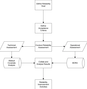
In the proposed reliability analysis model, it is assumed that subsea equipment or systems installed in the marine environment are subject to corrosion-induced degradation and human factor impact. A Weibull hazard rate relationship is derived and merged with a corrosion profile expression to produce the new reliability assessment model. Human and operation reliability are also evaluated using a barrier analysis method. Reliability analysis starts from definition of targets; however, actual quantitative assessment involves the following distinct tasks.

 Derive formulations for selected reliability assessment method.

 Calculate the basic scale and shape parameter of the failure data.

 Determine the Corrosion profile and Corrosion Weibull Reliability Index.

 Decompose system using Reliability Block Diagram and evaluate failure frequencies.

 Optimize system by analysing Fusell-Vesely reliability importance of components

based on failure frequencies and achievable reliability.

 Evaluate human-factor reliability using Barrier and Operational Analysis (BORA)

method.

Fig 1: Flowchart of Reliability Assessment Process.

2.1 Mathematical Formulation of Weibull Hazard Rate Model.

The basic Weibull model assumes that the family of the equation has two parameters where a basic failure rate of a distribution can be expressed as [13].

(1)

Wherein the constant α represents the scale parameter which is often termed the characteristic life of a system because it rates the time variable t with constant β representing the slope of the distribution as it determines the shape of the rate function.

Stochastically, the first failure can happen before the expected number of failures reaches 1, thus the need to select an appropriate benchmark time between failures.

Given a population of n components, with each possessing the same failure density f(t), the probability for each individual component failing by time F(tm ) is

(2)

Denoting the failure probability value by , the probability that certainly j components failed and (n− j ) did not fail at time tm is

; 1 (3)

It then follows the Median Rank which is the probability of j components or more failing at the time tm is given by

03 04

(4)

This is also known as the median rank formula.

On deriving the natural log of the two sides and negating we get

ln 1

1

(5)

Then taking the natural log again, we have

ln ln 1

1 ln ln

(6)

To illustrate the equations, assume a population of n has 100 components (at time t = 0), which has been in continuous operation. Assuming the first failure occurs at a time t = t1, then the estimated number of failures at the time of the first failure equals 1 [13]. This means that

F(t 1) = N(t1)/n = 1/100.

by [38] gives model parameters of shape (β), scale (α) and intercept (b) which are used to estimate the hazard rate. The hazard or survival rate of an item is a measure of the probability of an item to fail at about a specific time t, in the presence of a covariate factor c, provided it has been available up to time t [39]

Hence the hazard rate considering the covariate factor c, is defined as [38]

, lim

∆ →

∆ | ,

∆

(7)

If t represents time to failure. Then the hazard rate can be expressed as

, (8)

where cα = c1α1 + c1α1…. crαr, and α is the regression coefficient of the corresponding r

covariates. It then follows that when 1, the covariate factor c = 0 and Equation (8) will give the hazard rate So(t) [40].

The function can represent a wide range of functions, although it is considered an exponential function made up of product of the regression coefficient and the covariate. Since the reliability assumes a Weibull distribution, the hazard rate in the presence of covariate can be expressed as

, (9)

where λ and β are scale and shape parameters in the order laid out. If / , the hazard rate can be rewritten as

,

2.2 Model Formulation of the Weibull Corrosion-Covariate Stressor

The corrosion covariate profile entails physical parameters such as marine pH, temperature and CO2 pressure which are the key forces that affect an asset wear-out curve based on corrosion. The effects of corrosion whether external, internal or uniform are widely known to cause wear, fatigue and leakage. The extrapolation of regression analysis results beyond available data range requires accurate, justified, and tested covariate-life models [34][40]. To model the system in full water-wet condition, the Norsok’s Corrosion profile model was adopted and merged with the developed Weibull hazard expression guided by the principle of Arrhenius reaction model for accelerated life reliability analysis.

The Norsok corrosion model was chosen as the covariate factor because an increase in the CO2 partial pressure usually results in a drastic increase in the corrosion rate, a behaviour that is enhanced with temperature and causes the major degradation (failure) of both steel and non-steel units of the subsea compression system. It is a reliable physical relation developed, tested and proven to represent the oxidizing and corrosive impact of physical factors such as (CO2) partial pressure, temperature and flow [41].

The corrosion profile relationship for a deep water asset located in a zone with temperature 5 can be estimated using;

. ₍₁₁₎

The Arrhenius asset life model is governed by the principle that life of a system is directly proportional to the inverse reaction rate. The Arrhenius equation is given by [40].

(12)

L signifies a quantifiable life measure while V stands for the covariate factor, developed for thermal-corrosion related variables in absolute units. C and b represent model parameters which can be calculated from analysis of variance of data.

If scale parameter is regarded as a function of the covariate, then hazard rate, h becomes,

,

(13)

Since temperature profile could give a life measure, it also makes sense for a corrosion profile stress to be part of the life covariate functions. On substituting the corrosion profile variable v into the survivability equation, system hazard rate under the influence of corrosive stress becomes,

,

(14) 

Reliability can thus be expressed as,

,

(15)

Reliability can also be expressed as a function of

1

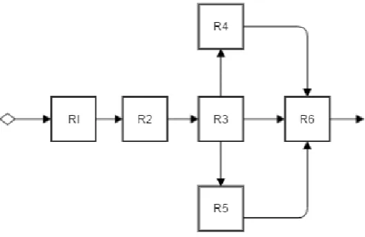
2.3 Decomposition with Reliability Block Diagram (RBD) and Optimisation

the complex connections and reliability interactions of the system’s components.

Fig 2: A typical system with both series and parallel relationships.

2.4 Reliability Optimisation

To develop an optimisation model, consider a system with x amount of components and the target is to optimize reliability to meet reliability without over-designing certain components to the detriment of other critical ones to minimise cost.

The optimality factor is the ratio of targeted reliability index for a system and its weibull-corrosion covariate reliability index multiplied by the failure time or basic Mean Time to Failure

(MTTF) of a system.

Mathematically, Optimality factor (OF) is,

(17)

The reliability importance ( ) of a system is defined as the ratio of system reliability

overall reliability. Mathematically, Reliability Importance (IR) is expressed as [42].

The Benchmark Minimum Failure (Minimum MTTF) can also be estimated and this refers to the product of the optimality factor and the reliability importance of a component. It is an expression that is used to arbitrarily extract resources from the over-designed components and evenly add to the under-designed or early failure ones. Two assumptions are made when evaluating the minimum time to failure.

 An assumption that if a component’s life expectancy is more than three standard

deviations beyond the statistical control limits (especially if beyond upper control limits) of the unstressed failure distribution, then the excess life would be extracted from the over-designed component and evenly shared among less reliable components within a sub-system.

 If the reliability importance of a component is 0 or less than 0.1, the minimum time to

failure remains the same as unstressed failure data. (See table 5 )

Optimal Time to Failure (Optimal MTTF) is gotten by dividing-up the extracted life values obtained from over-designed among other components, thereby optimizing and extending its life to failure.

2.5 Human-factor Analysis.

reliability analysis. These include, methods such as Technique for Human Error Rate Prediction – THERP, Human Error Assessment and Reduction Technique – HEART, Success Likelihood Index Method Multi-attribute Utility Decomposition – SLIM-MAUD and more recent techniques which are often referred to as second generation, or advanced methods such as Cognitive Reliability and Error Analysis Method – CREAM, Standardized Plant Analysis Risk Human Reliability Analysis – SPAR-H, Information, Decision and Action in Crew context – IDAC, in addition to probabilistic ones such as Bayesians models [2][3] , Organisational Risk Influence Model- ORIM, Model of Accident Causation using Hierarchical Influence Network-MACHINE. The major challenge is that many of these models with the exception of [2][3] were not particularly designed with reference to offshore risk inputs and industry average occurrence rate of those accidents[16][55].

The method employed for human factor analysis in the paper is a simplification of the Barrier and Operational Risk Analysis (BORA) model by [16] which is a very comprehensive framework for modelling and optimising barriers on offshore production installations. The introduction of severity measure in this paper is a major enhancement of the BORA methodology because it readily compares and presents the monetary consequence of impeding system risk. Industry average probability was decided by calculating the mean of participant’s rating for each category. The status of these factors for the specific oil field was also obtained in the same manner.

corrosion covariate expression.

In line with BORA recommended approach, the formula for calculating the revised Risk Influencing factor P(rev) is given by [16] [43].

∑ (19)

where Pave (X) represents the industry average of probability of occurrence of an event X,

Wi is the weight allocation of the Risk influencing factor and Qi represents an actual measure

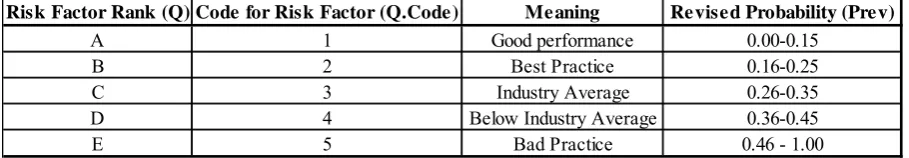
of the status of Risk influencing factor at field. The severity of the Risk Influencing Factor (RIF) is ranked on a scale of A to E with A (representing outstanding practice in Industry) to E (Worst practice in industry) where C corresponds to industry average. Table 1 summarises all the input data, rating system and weights applied to the risk influencing factor and the adjustment ratio.

Table 1: Risk Factor Code Table

The modification factor (MF) depends on the product of allocated weights (Wi) and rated event probability (Qi).

(20) 

The weights are applied relative to the importance of each factor on scales 0.2, 0.4, 0.6, 0.8 Risk Factor Rank (Q) Code for Risk Factor (Q.Code) Me aning Re vised Probability (Prev)

A 1 Good performance 0.00-0.15

B 2 Best Practice 0.16-0.25

C 3 Industry Average 0.26-0.35

D 4 Below Industry Average 0.36-0.45

and 1.0; where 0.2 means the least importance/influence and 1.0 meaning the utmost importance. Event probability (Q) is rated using a scale of A-E as shown in Table 1. The true value for the technical reliability index obtained from the new model is weighted together with the interview data obtained from survey for all factors in each category.

3. Case Study

The purpose of this case study is to demonstrate the applicability of the new model developed in Section 3 for reliability analysis and optimisation of a subsea compression system.

3. 1 Description of the case

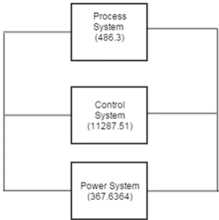
A major oil and gas firm wants to conduct a reliability assurance analysis on a subsea gas compression system proposed for the installation at the Escravos field off the coast of Nigeria, West Africa. The target reliability is 95% for the initial 300 days. To support decision making processes, the firm had requested for a numeric quantity of the subsea system’s survivability under operational stresses. The system which is directly synchronized with power units, a process system and control system is meant to take reservoir gas from the wellhead, through the compression system to a centrally positioned FPSO. The compression unit performs the mechanical job of compressing well fluid while the power units provide electric power for the entire system. The control system conveys and receives sensor signals between the Subsea Engineers on deck.

3.2 Case Analysis -Weibull-Corrosion Covariate Reliability Analysis

certain defined time. Majority of the failure data were obtained from OREDA [54]. Prior to the regression analysis of the MTTF data, some adjustments were performed to make the distribution a Weibull distribution. Firstly, the failure data is ranked in descending order as shown in the column ‘Rank’ of Table 2. The median rank for failure is then calculated to ascertain the proportion of the system component that will fail by the mean time in column MTTF.

Using the Bernard’s equation for determining median rank [13]: 0.3

0.4

(21)

where X represents the column rank and N is the sum of failed components being considered . In this case, there are 39 components as shown in Table 2.

The median rank and MTTF are further transformed by taking their natural logs using Eq. 5 and repeated with equation 6; so that regression analysis can take place more efficiently. A simple linear regression analysis is performed between ‘In MTTF’ and ln(ln(1/(1-Median Rank) in order to obtain parameter estimates in determining the survival rate.

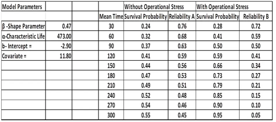
The scale parameter and the shape parameter are obtained from linear regression analysis [47] of In(In(1-Median Rank)) and In MTTF columns in table 2 above. The coefficients obtained are 473.36, 0.47 and the intercept -2.9.

The Weibull scale parameter (α) was obtained by substituting the b and β in Equation (22).

(22)       

In line with Weibull’s principles, the characteristic life indicates the time at which 63% of system components would have failed irrespective of the value of [12][13]. With an assumption that MTTF is expressed in days, the results from regression analysis indicate that at 473.36 (days), the unstressed reliability of the system in the absence of any repair or replacement work would be 37%.

No SUBSEA COMPRESSION SYSTEM MTTFSOURCE Rank Rank1Median Rank 1/(1-Median Rank ln(ln(1/(1-Median Rank)) ln(MTTF) Process System

1 Manifold Piping 3,048 OREDA 5.6 1 0.017766497 1.018087855 -4.021491042 1.7227666

2 Mechanical Connector 1,351 OREDA 6.1 2 0.043147208 1.045092838 -3.121165758 1.80828877

3 ROV Isolation Valve 1,389 OREDA 6.3 3 0.068527919 1.073569482 -2.645229481 1.84054963

4 EI Isolation Valve/Actuator 1,489 OREDA 7 4 0.093908629 1.103641457 -2.316530606 1.94591015

5 Check Valve 162 OREDA 8.1 5 0.11928934 1.135446686 -2.063362471 2.09186406

6 Scrubber 50 OREDA 9 6 0.144670051 1.169139466 -1.856182932 2.14006616

7 Scrubber Level Detector 98 Tracerco 24.5 7 0.170050761 1.204892966 -1.679910065 3.19867312

8 Magnetic Bearing System Compressor 27 S2M Report 27 8 0.195431472 1.242902208 -1.525790316 3.3068867

9 Compressor 9 OREDA 32 9 0.220812183 1.283387622 -1.388283692 3.4657359

10 Electric Motor(Compressor) 5.6 Aker Solution 38.7 10 0.246192893 1.326599327 -1.26365639 3.6558396

11 PSD Sensors 124 OREDA 41 11 0.271573604 1.3728223 -1.149267807 3.71357207

12 Flow Meter for Anti Surge Control 650 OREDA 43 12 0.296954315 1.422382671 -1.043177384 3.76120012

13 Anti Surge Actuator 228 Aker Solution 50 13 0.322335025 1.475655431 -0.943913114 3.91202301

14 Anti Surge Valve 89 OREDA 70 14 0.347715736 1.53307393 -0.850327856 4.24849524

15 Cooler 84 OREDA 84 15 0.373096447 1.5951417 -0.761506169 4.4308168

16 Condensate Pump Unit 6.1 KOP 89 16 0.398477157 1.662447257 -0.676701617 4.48863637

17 Re-circulation choke valve 32 OREDA 89 17 0.423857868 1.735682819 -0.595293163 4.48863637

18 Meg Piping 309 OREDA 98 18 0.449238579 1.815668203 -0.516753902 4.58496748

19 Pressure and Volume Controller 89 OREDA 100 19 0.474619289 1.903381643 -0.440627964 4.60517019

Control System

20 Top Side Master Control Station 24.5 OREDA 108 20 0.5 2 -0.366512921 4.68213123

21 Wet Mate Connector 24980 OREDA 124 21 0.525380711 2.106951872 -0.294045889 4.82028157

22 Electrical Dry Mate Connector 4424 OREDA 162 22 0.550761421 2.225988701 -0.222892112 5.08759634

23 Electric Jumpers 72022 Teledyne 192 23 0.576142132 2.359281437 -0.152735069 5.25749537

24 Junction Boxes 41 Telecordia 228 24 0.601522843 2.50955414 -0.083267372 5.42934563

25 Magnetic Bearing Control Module 6.3 S2M Report 309 25 0.626903553 2.680272109 -0.014181765 5.73334128 26 Anti-Surge Compressor Control Pod 38.7 CFD DOC 310 26 0.652284264 2.875912409 0.054838487 5.7365723

27 SCM 43 OREDA 358 27 0.677664975 3.102362205 0.124130689 5.88053299

28 UPS 8.1 OREDA 554 28 0.703045685 3.367521368 0.19406646 6.31716469

Power System

29 Topside Main Circuit Breaker 1116 OREDA 554 29 0.728426396 3.682242991 0.265069889 6.31716469

30 Topside Transformers 554 Vetco Gray 650 30 0.753807107 4.06185567 0.33764293 6.47697236

31 VSD 7 OREDA 675 31 0.779187817 4.528735632 0.412402847 6.51471269

32 Topside Umbilical Hang-off 358 OREDA 1116 32 0.804568528 5.116883117 0.490140445 7.01750614

33 Power Umbilical 108 OREDA 1,351 33 0.829949239 5.880597015 0.571915995 7.20860034

34 Umbilical Termination Assembly(UTA) 310 OREDA 1,389 34 0.855329949 6.912280702 0.659228202 7.23633934

35 Subsea Enclosures (Transformer) 675 OREDA 1,489 35 0.88071066 8.382978723 0.754337905 7.30586003

36 Subsea Main StepDown Transformer 554 Vetco Gray 3,048 36 0.906091371 10.64864865 0.86096109 8.02224092

37 Hv Penetrator/Dry Connector 192 Deutch 4424 37 0.931472081 14.59259259 0.986008583 8.39479954

38 Hv Power Jumper 100 OREDA 24980 38 0.956852792 23.17647059 1.145221526 10.1258308

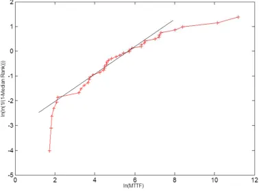
To check the fitness of Weibull 2-parameter modelling for analysis, a line fit plot as shown in Fig 3 between failure values and the natural log of the median is generated.

Fig 3: Line Fit plot showing fitness of data for reliability analysis

On close observation of fig 3, the fitted line has little doglegs which show that the failure modes affecting the system come from various origins [46]. In the current case, these can be overlooked because such scatter plot is typical for the hydro-mechanical components. The OREDA failure data being used generates such shape parameter of the failure distribution as supported by [46][47] provided that the straight line slope of such plot gives the shape parameter of the distribution. The plot has shown that the Weibull distribution modelling is a good choice and the generated values fit properly with theoretical values.

of the external influential forces that could interfere and further reduce system reliability. Values of the boundary variables were obtained from experts at the Egina field Nigeria. The temperature profile for West African waters is shown in Fig 4.

Fig 4: Temperature Profile for a West African Offshore Field [48]

The corrosion profile, for the subsea compression system was obtained using (reference of the following equation):

. ₍₂₃₎

If the water depth 1500 meters, Temperature Constant at 5 degrees Celsius KT = 0.42 [41]; FCO2 = Fugacity of CO2 pressure = 5840psi = 40265kPa (Field data);

F = Fugacity of pH at West African Water at pH 9 = 0.2208 (Field data) Therefore, 11.8

Having generated a covariate parameter to represent the influence of marine conditions, next step is to estimate the overall reliability index of the SCS system using Equation 15 as shown below containing the values of the shape and scale parameters derived from the failure data:

,

2.9 _.

473

. ₍₂₄₎ 

20 15 10 5 2500 2000 1500 1000 500 0

Te mpe rature (Celsius)

W a te r D e p th (M e te rs )

A stressed survival signature has been proven to be an effective method to estimate the survival function of systems with multiple component [42] and table 3 shows the values for both stressed and unstressed failure data using the new failure model. The contribution to unreliability by each failure data is taken into account and as a consequence, bounds of survival functions of the system and ratings of relative importance index values can be obtained using further optimization analysis.

Fig 5: Basic Weibull failure vs Stressed Weibull-Corrosion failure.

The result in Table 3 and Fig 5 show the impact of marine physical conditions on failure rate. The asset-life decline curve obtained from the stressed Weibull-covariate model gave a steeper decline curve compared to the unstressed Weibull failure model. This result further confirms that a catastrophic infant mortality is imminent if the quality and redundancy configurations of the components are not improved.

3.3 Root-Cause Analysis using Reliability Block Diagram.

Boolean algebra expressions defined by the MTTFs data of each component from table 2 are used to determine minimal cut sets or the minimum combination of failures required to cause a system failure. The RBD calculates system failure frequency and unavailability based on the Vesely model. The fundamental law guiding the analysis using ITEM software used for the RBD decomposition is the Weibull failure distribution principle and an extrapolation of failure data by the Vesely theory [49].The rationale guiding the combination of both laws is the assumption that there are no repairs thus failure is assumed as an exponential degradation

300 250 200 150 100 50 0 0.8 0.7 0.6 0.5 0.4 0.3 0.2 0.1 0.0

Time (days)

R e lia b ilit y I n d e x Unstressed Failure

curve. All failures are statistically independent. The failure rate of each subsea component is constant. After repair, the system will be as good as old, not as good as new based on the Weibull distribution model being applied. All component failures are statistically independent. The failure rate of reach equipment item is constant. The repair rate for each equipment item is constant. After repair, the system will be as good as new, (i.e., the repaired component is returned to the same initial state, with the same failure characteristics that it would have had if the failure had not occurred; repair is not considered to be a renewal process [49].

Let component failure rate be,

1 (25)

1 (26)

(27)

/ (28)

Where represents time specific unreliability of the system, is the time specific

recovery frequency of the system , time-specific failure frequency of the system, is the time specific failure rate of the system, the time specific recovery rate of the system, K is the phase of minimal cut set and t is time. More detailed derivation can be found in Jincheng [49].

The Fusell-Vesely measurement highlights an event’s contribution to system unavailability because it gives an idea on the likelihood that a component is down because a system is down. It is very important to identify those components in a system which have the greatest impact

on overall system reliability. In practice, this is done by first choosing a suitable measure

of component importance, calculating them for each component and then ranking the

importance of components according to that measure. In this paper, a presentation is made

of the various results for the power, process and control systems. This can be used to

importance measures so that the components can be ordered by their structural criticality.

These results help to quickly estimate optimizable components, because calculating the

exact values of the component importance measures is very laborious in a large and

complex system [50].

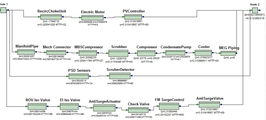
The RBD analysis was based on an enhanced Vesely theory which allowed the allocation of reliability capabilities to each block based on the logical failure of the system with respect to series and parallel connections. Fundamentally, the RBDs offer a higher probability of dangerous failure than other advanced techniques [19]. In this study, it was applied to model and decompose the system failures into cut-sets in order to visualize how the system is set-up and measure the actual faulty components so that a good logic for their optimization analysis will suffice rather than using a generic fault tree which is more suitable for sensitivity analysis without optimization details. It should be noted that it was used in a different way in the present analysis to consider the cut-sets on a node by node basis of process, control and power sub-systems. The clear advantage is that it simply allows the software’s failure estimation rule to analyse the contribution of each component to unreliability.

Fig 6: Reliability Block Diagram of the Subsea Compression System

3.3.1 Reliability Analysis of the Process Sub-System

The process sub-system is the section of the subsea compression plant where actual separation well fluid and compression of gas occurs. An RBD diagram of the process sub-system is cut out from the main subsea compression sub-system and calibrated accordingly with the MTTF values of Table 2. A simulation is run using ITEM Reliability Software for a lifetime of 7200 hours or 300 days and an average MTTR of 7 applied to each component. The component failure data is fed to the system. 100 iterations are run on each sub-system as obtained from Piping and instrumentation drawings to determine the severity index and reliability importance of the components. This iteration is repeated for all the sub-systems. The failure severity index measures the intensity of unreliability of each sub-system

The Failure Severity index is mathematically expressed as

x x (29)

Where T represents Time, represents Failure frequency and represents Expected failures.

and their various reliability importance for adequate system optimization. Fig 7 shows the reliability blocks configuration into a mix of series and parallel cut-sets as obtainable in realistic configuration.

Fig 7: Reliability Block Diagram (RBD) of SCS Process Sub-System

Fig 8: Time vs Unreliability for Process Sub-System

The time and unreliability index graph shown in Fig 8 indicates that the unreliability of the process components rapidly increases and attains full unreliability value in 288 days which significantly deviates from the target benchmark of 300 days or 7200 hours. The reliability of this system in relation to target operation benchmark is zero, therefore, all the critical components need to be optimized.

1600 1400

1200 1000

800 600

400 200

0 1.0

0.9

0.8

0.7

0.6

0.5

0.4

0.3

Me an Time Ste p

U

n

re

lia

b

ilit

y

I

n

d

e

x

(

%

Fig 9: Reliability Importance for Process Sub-system Components Systems.

Figure 9 shows the reliability importance chart of process components. To identify the critical components which need reliability upgrade the most, another analysis is subsequently run using Fusell-Vesely’s equation (FV). Fussell-Vesely Importance of the modelled plant

feature (usually a component, train, or system) is defined as the fractional decrease in total risk level (usually CDF) when the plant feature is assumed perfectly reliable (failure rate = 0.0). If all the sequences comprising the total risk level (e.g. CDF) are minimal, the F-V also equals the fractional contribution to the total risk level of all sequences containing the (failed) feature of interest. Where F-V = 1-1/RRW and RRW is Risk Reduction Worth (RRW) [51].

Change in unavailability of events with high importance values will have the most significant effect on system unavailability.

∑

(31)

Fig 9 above shows that the Meg Piping with zero reliability importance index, Mechanical MEG Mech Conn ecto r; ROVI soVa lve; FMSu rgeC ontro l; PVCo ntroll er; AntiS urge; Chec kValv e; Cond ensa tePum p; PSDS enso r; Electr icMot or; 0.7 0.6 0.5 0.4 0.3 0.2 0.1 0.0

Proce ss Compone nts

connector and Isolation Valve contributes least to unreliability while the electric motor with an importance factor of 68%, the PSD Sensor and condensate pump are top contributors to frequent failure of the process sub-system. A trade-off on cost will then guide the choice of redundancy or quality improvement to be made on the components.

3.3.2 Analysis of the Control Sub-system.

The control sub-system entails the auto-sensory segment which continuously monitors the overall condition of the subsea compression plant. In (Fig 10), the system is wired-up in reliability configuration and reliability analysis simulation is run through on the cut-sets.

Fig 10: Reliability Block Diagram (RBD) of the Control Sub-System.

Fig 11: Time vs Unreliability of the Control Sub-System

The control system chart in Fig 11 appears to be the main contributor to failure being that complete unreliability was reached within 72 days. The system fails rather earlier than the benchmark target therefore a further investigation to identify the contributors is justified. Recall some components in this sub-system has the highest MTTF with Wet Mate Connector and Electric Jumpers having 24980 and 72022 MTTFs respectively according to table 2. This analysis reveals that a high MTTF does not directly translate to high reliability rather the cumulative MTTFs together with frequency and times of failure gives better prediction of system reliability.

400 300

200 100

0 1.0

0.8

0.6

0.4

0.2

0.0

Me an Time Ste p

U

n

re

lia

b

ilit

y

I

n

d

e

x

(

%

Fig 12: Reliability Importance for the Control Sub-system.

Fig 12 shows that the Subsea Control Module (SCM) and the Dry Connector did not contribute much to unreliability rather it the Master Control and UPS that are critically important to overall system reliability because they contribute to unreliability by 32% and 68% respectively.

This implies that a significant upgrade of these two components will significantly improve the reliability of the control system cut set.

SCM MBCo ntrolM od, Juncti onBo xes, AntiS urgeC ontro l, Electr icJum pers, WetM ateCo nnec tor, DryC onec tor, Maste rContr ol, UPS, 0.7 0.6 0.5 0.4 0.3 0.2 0.1 0.0

Control Syste m Compone nts

3.3.3 Analysis of the Power Sub-System

The power system supplies the electric voltage that runs the subsea compression system. It is an integral part of the system that runs from the top side through the umbilical cable down to the base of the ocean where the compressor is located. Arhenius Law and Basquin Law posited that electronic components fail due to an increased ambient temperature [52]. It is possible to extend the life of the power components beyond the mean MTTF using pressure protective enclosures for the power sub-components as demonstrated by [53], however this particular research seeks to identify how the system configuration contributes to reliability and failure severity for stochastic optimisation. This implies that temperature fluctuations underwater have serious impact on the lifespan of the power sub-components. To account for this, the model law assumes a uniform fatality constant for stress based on the Weibull reliability index earlier estimated in 3.2. Fig 13 below shows that the decomposition and of power system in series connection based on instrumentation diagrams obtained for the case study.

Fig 13: Reliability Block Diagram (RBD) of the Power Sub-System

to be the most reliable and of least reliability importance. The failure frequency was 0.167% for the sum of total number of expected failures was 0.176. The severity index was found to be 0.002 disregarding the fact that it had 11 cut-sets.

Fig 14: Time Vs Unreliability of the Power Sub-system

The power sub-system is the least contributor to failure of the whole subsea compression system being almost 99.9% of reliability was maintained further in time step than other sub-systems. Fig 14 shows that, at maximal unreliability, the system maintains a total unreliability of 0.18 in 1 time step. System unreliability is relatively low and varies almost linearly with time. The three data points on Fig 14 established a sufficient convincing trend, however, in real field applications; curve fitting may be exercised on the graph to determine the best-fit decision for reliability improvement.

1.0 0.8

0.6 0.4

0.2 0.0

0.20

0.15

0.10

0.05

0.00

Time Ste p

U

n

re

lia

b

ilit

Fig 15: Reliability Importance of the Power Sub-system

The Variable Speed Drive (VSD) was identified as the critical item to be improved in the power segment. The high voltage connector may also need to be optimized, because, under subsea operational circumstances, the failure rate would increase. Table 4 shows a break-down of the results from sub-systems reliability assessment. Table 4 showcases the severity table of the whole system based on the Weibull analysis and Fusell-Vesely of the minimal cut sets. Minimal cut sets depend on the number of blocks in connection in each sub-system. A two-tailed F-test reveals that there is no relationship between the number of cut sets and expected failure, reliability, unreliability and failure frequency but there seems to be relationship between number of cut sets and severity. Thus, the lower the cut sets, the higher the severity. The biggest contributor to severity factor is total downtime.

TCirc uitBr eake r Subs eaTra nsfo rmer TopT ransfo rmer Umbil icalTe rmAs sy HVDr yCon necto r Powe rUmb ilical HVPo werJu mper HVW etCon necto r VSD 0.8 0.7 0.6 0.5 0.4 0.3 0.2 0.1 0.0

Powe r Compone nts

Table 4: Summary Table of Sub-Systems Reliability

3.4 Optimisation of the Subsea Compression System

Optimisation of the whole Subsea Compression System requires a careful consideration of the Weibull-Corrosion Covariate results of table (3) and table (4).

Since basic Weibull analysis has showed an infant mortality failure, it is imperative that the design is optimized to achieve the necessary reliability levels. Based on the requirement of 96% reliability at 300 days, a close look at the system components’ MTTF indicates that that up to 25 components were under-designed while 14 were over-designed. The low survivability of majority of the individual components was responsible for the low value of β and the subsequent stress induced failure.

An optimisation of the lope-sided reliability design can be achieved by enhanced process control at the design stage and subsequent identification of reliability importance of the

various components. Fig 16 shows the process control chart of the system.

Subsea Compression Sub-Systems No of Cut Sets Unreliability (%) Reliability (%) Total Downtime Expected Failures Failure Frequency Severity

Process System 19 1 0 156.64 88.5 0.0123 170.51

Control System 9 1 0 4180 496 0.0685 142019.68

Fig 16: Statistical Process Control Chart for Design Optimisation

System optimization using control charts helps to identify design needs from a cumulative perspective. In Fig 16, it can be observed that the design violated the seven-point rule which suggests that seven consecutive data points above or below the mean indicates a problem with the process. With a mean MTTF of 2945 as benchmark, a standard deviation of the mean (CL) 2945 gives an upper control limit (UCL) and a lower control limit (LCL) of 39703 and -33182 respectively. There is then room for process-smoothing and possibly cost balancing as these will help to prevent the discrepancy resulted from either over-design or poor designs. Whole failure time of any components that falls out of the standard limits would need to have some of its value extracted and shared out to deficient components in the distribution. This further confirms that unavailability of the subsea compression system under review is due to poor design and process control of individual components therefore there is a need for further analysis of the sub-systems and components to trace the key contributors to unreliability.

40 30

20 10

0 80000

60000

40000

20000

0

-20000

-40000

Equipment Number

T

im

e

t

o

Fa

ilu

re

MTTF DATA CL

Table 5: Optimized Subsea Compression System

Table 5 shows the optimisation of the subsea compression system to maintain 96% reliability at 300 days. The RBD decomposition of the entire system into its constituent components and analysis with pre-set algorithms in the ITEM software helped to analyse the contribution of each component to overall reliability. Whilst some components needed an increase MTTF, others for instance No (13), (Electric Jumpers) had way too much uptime life and its optimal MTTF had to be smoothened to a lower value to accommodate other deficient components. The components whose reliability importance are 0 or less than 0.1 are left untouched as seen in No (1), (Manifold Piping) in Table 5 where 3048 was both the initial MTTF and minimum MTTF but only increased to 3877 by taking a percentage of the extracted excess life of the

No SUBSEA COMPRESSION SYSTEM Initial MTTF Optimality Factor Reliability Importance Minimum MTTF Optimal MTTF Process System

1 Manifold Piping 3,048 58,522 0 3,048 3,877

2 Mechanical Connector 1,351 25,939 0 1,351 2,180

3 ROV Isolation Valve 1,389 26,669 0.04 1066.752 1,895 4 EI Isolation Valve/Actuator 1,489 28,589 0 1,489 2,318

5 Check Valve 162 3,110 0.25 777.6 1,606

6 Scrubber 50 960 0.12 115.2 944

7 Scrubber Level Detector 98 1,882 0.56 1053.696 1,882 8 Magnetic Bearing System Compressor 27 518 0.32 165.888 995

9 Compressor 9 173 0.43 74.304 903

10 Electric Motor(Compressor) 5.6 108 0.69 74.1888 903

11 PSD Sensors 124 2,381 0.44 1047.552 1,876

12 Flow Meter for Anti Surge Control 650 12,480 0.08 998.4 1,827

13 Anti Surge Actuator 228 4,378 0.18 787.968 1,617

14 Anti Surge Valve 89 1,709 0.44 751.872 1,581

15 Cooler 84 1,613 0.08 129.024 958

16 Condensate Pump Unit 6.1 117 0.44 51.5328 880

17 Re-circulation choke valve 32 614 0.22 135.168 964

18 Meg Piping 309 5,933 0 309 1,138

19 Pressure and Volume Controller 89 1,709 0.11 187.968 1,017 Control System

20 Top Side Master Control Station 24.5 470 0.32 150.528 979

21 Wet Mate Connector 24980 479,616 0 24980 25,809

22 Electrical Dry Mate Connector 4424 84,941 0 4424 5,253

23 Electric Jumpers 72022 1,382,822 0 39703 39,703

24 Junction Boxes 41 787 0 41 870

25 Magnetic Bearing Control Module 6.3 121 0 6.3 835 26 Anti-Surge Compressor Control Pod 38.7 743 0 38.7 867

27 SCM 43 826 0 43 872

28 UPS 8.1 156 0.67 104.1984 933

Power System

29 Topside Main Circuit Breaker 1116 21,427 0 1116 1,945

30 Topside Transformers 554 10,637 0 554 1,383

31 VSD 7 134 0.72 96.768 925

32 Topside Umbilical Hang-off 358 6,874 0 358 1,187

33 Power Umbilical 108 2,074 0 108 937

34 Umbilical Termination Assembly(UTA) 310 5,952 0 310 1,139 35 Subsea Enclosures (Transformer) 675 12,960 0 675 1,504 36 Subsea Main StepDown Transformer 554 10,637 0 554 1,383 37 Hv Penetrator/Dry Connector 192 3,686 0.02 192 1,021

38 Hv Power Jumper 100 1,920 0.05 100 929

Electric Jumpers.

3.5 Human-Factor Reliability Assessment

A questionnaire based on the Delphi method was developed by interviewing experts from the West African subsea sector. The questionnaire was reviewed by a reference panel to confirm its academic and ethical status. The panel was made up of engineering experts whose backgrounds were operation, maintenance, and subsea engineering.

A pilot survey was launched and little adjustments were effected on the final draft before the proper interview was carried out. The first section of the interview was designed to discover the company’s main business activities, experience and technical know-how of the respondents and in order to understand how the operations are shared-out within the company while at the second section, the company’s subsea personnel were required to highlight its strategy for offshore system maintenance activities and the operational challenges at play. Their opinions were measured on a scale and the same questionnaire was used in order to maintain uniformity of data from participants.

Five key factors were analysed being that they are factors during the installation, production and maintenance stages of a typical West African oil field. Ten specialists were interviewed through phone calls. Five of the specialists work with operators, two specialists work with subsea manufacturing companies and the other two specialists work with a company providing subsea consultancy service.

Each of the specialists possess a minimum four years’ experience with subsea systems and at least 10 years’ experience in several engineering and management positions within the subsea oil and gas industry. Based on the respondents’ profiles, the study reasonably indicated current trends and rating regarding human factor and operation indices of subsea oil and gas production practices, problems and issues in the installation.

fed to the slot for the technical condition/reliability system and the severity code read-off. The revised probability of failure in Tables 5 and 6 show that the most contributing Risk Influencing Factor (RIF) is personnel factors with a 56% probability of failure and the overall least RIF is technical factors with a 29% probability of occurrence. The severity index could be transcribed into weighted financial consequences from depending on pre-set benchmarks. From the results, urgent effort needs to be made towards smart resource allocation and staff scheduling in order to reduce human fatigue risks, improve occupational health and safety, and associated cost implications. Whilst the sum of Revised Probability (Prev) of Influence for the technical RIFs seem to be relatively low due, a look at the modification factor shows that elements such as material properties and process complexity of the system were both significantly high at 1.2, thus, requires improvement. Table 6 entails an enhanced method for human reliability assessment for quantitatively assessing the risk in a particular scenario.

Table 6: Human Reliability Analysis Table

Table 7: Risk Matrix Table of the RIFs No RISK INFLUENCE FACTOR

Industry Average (Pave) Weight (W) Risk Influencing Factor (Q)

Code for Risk Influencing Factor (Q. Code)

Moderation Factor (MF)

Average Moderation Factor (MF Ave.)

Revised Probability (Prev)

1 PERSONNEL FACTORS 0.45 1.25 0.5625

1a Competence 0.8 C 3 2.4

1b Work Stress 0.2 D 2 0.4

1c Fatigue Rate 0.2 D 2 0.4

1d Health Condition 0.6 C 3 1.8

2 TASK FACTORS 0.44 1.01 0.4463

2a Ergonomics 0.5 C 3 1.5

2b Supervision 0.2 C 3 0.6

2c Methodology 0.4 D 2 0.8

2d Time Pressure 0.8 E 1 0.8

2e Sufficient Work Tools 0.2 D 2 0.4

2f Spares Availability 0.2 C 3 0.6

2d Explosivity/Inflamability 0.8 C 3 2.4

3 TECHNICAL ELEMENTS 0.37 0.77 0.2854

3a Equipment Design 0.2 C 3 0.6

3b Material Properties 0.4 C 3 1.2

3c Process Complexity 0.4 C 3 1.2

3d Human Machine Interface 0.2 D 2 0.4

4d Maintainability 0.2 D 2 0.4

5e System Feedback 0.4 D 2 0.8

5f Technical Condition/Reliability 0.8 E 1 0.8

4 ADMINISTRATIVE 0.33 1 0.33

4a Work Permit 0.2 C 3 0.6

4b Work Safety Analysis 0.4 C 3 1.2

4c Procedures/Protocols 0.4 C 3 1.2

5 OPERATIONAL PHILOSOPHY 0.35 1.16 0.406

5a Trainings 0.6 C 3 1.8

5b Enterprise Feedback Loops 0.4 D 2 0.8

5c Communication 0.6 C 3 1.8

5d Regulation 0.4 D 2 0.8

5e Management of Changes 0.2 C 3 0.6

RATING

10 20 30 40 50 60

i Personnel Factor ii Task Factor

iii Techanical Elements iv Administrative

v Operational Philosophy

Se ve rity Inde x(Pe rce ntage )

3.6 Strengths and Limitations

 The key contribution of the research is a new systematic methodology for stressing a

low-stress failure data such as OREDA MTTF in order to predict a realistic failure curve and optimize an asset which has little field records but bound to face exponential covariate vectors of operational stresses afield.

 To model the reliability of a system in full water-wet condition, the Norsok’s Corrosion

profile model was adopted and incorporated with the newly developed Weibull failure expression by implementing the principle of Arrhenius reaction model for accelerated life reliability analysis.

 The motivation of the current study is due to the unavailability of any known

publication which addresses the reliability and optimization of a Subsea Gas Compression System - an emerging technology that had only been launched in 2015 at Asgard field, Norway.

 Further development of the present reliability analysis method shows that the baseline

reliability index of a system were stressed with statistical stress based on intended operating environment, in this case corrosion profile considering extended parameters such as subsea temperature, pressure, pH and fugacity variables, so that weak components are identified and an optimal MTTF is proposed (either increased, kept constant or decreased) for each component as shown in Table 5.

to visualize the life failure data, accelerate failure life and project optimal tolerances for subsea equipment subjected to operational influences of both the marine and human factors. The corrosion-Weibull covariate model produced valid benchmark which is vital for the improvement of the overall design of the subsea compression system for longer life. Redundancies and back-up systems were not considered in this study however, the detailed statistical analysis of the system has a 95% confidence status.

4. Conclusion

This paper constitutes a step forward in the use of advanced qualitative and quantitative analysis for assessing the reliability of the emerging subsea compression system.

 This paper reveals that a high MTTF component does not directly translate to high

reliability of a system rather the cumulative MTTFs together with frequency and times of failure gives better prediction of system reliability.

 It is more efficient and time-saving to (a) identify any infant mortality (b) identify

over-designed components by applying Weibull failure model and Fusell-Vesely theory to their minimal cut sets for optimizing overall reliability index based on criticality and reliability importance of components. The initial basic reliability of the system was optimized by a margin of 52% from 0.45 to 0.95 based on the confidence interval of the whole reliability analysis.

 The operational requirements of a subsea gas compression system can be understood

and optimized by embedding a high operational stressor using a covariate corrosion profile on a weibull model of component failure distribution, then reliability decomposition of the sub-components to identify the critical components and an optimization analysis based on reliability importance of each sub-component.

 Low subsea temperatures, high Co2 fugacity and pH variation has a significant impact

on asset degradation rate, failure modes and frequency over a time series. Personnel factors such as competence of the operators, works stress, fatigue, stress, and ergonomics constitute the highest weight of risk influencing factors that could cause a subsea gas compression system – based on the geographical setting of the study.

 The new model demonstrated a significant originality in producing more realistic

failure rate compared to the basic reliability models which does not consider credible external influences.

The newly developed method in the paper combines the powerful calculative abilities of a Weibull with corrosion covariate model together with systematic decomposition of the whole system with RBD analysis, subsequent identification of the reliability importance of each component and the novel optimisation method therein.

References

[1] Skogdalen,J. Utne I.B., Vinnem J., (2011). Developing safety indicators for preventing offshore oil and gas deepwater drilling blowouts. Safety Science,

Volume 48: 1187–1199.

[2] Cai Baoping, Yonghon L, Zengkai L, Xiaojie T, Yanzhen Z, Renjie Ji, (2013) A Dynamic Bayesian Network Modelling of Human Factors on Offshore Blow outs, Journal of Loss Prevention in Process Industry, Volume 26, Issue 4, July 2013, Pages 639–649

[3] Vadachalam N., (2016 ). An Approach to Operational Risk Modelling and Estimation of Safety Levels for Deep Water Work Class Remotely Operated Vehicle - A Case Study with refrence to ROSUB 6000 . Journal of Ocean Engineering and Science, (2016) 1-10

[4] HSE, Health and Safety Executive, UK, (2014). Offshore Technology Report:Review of Corrosion Management for Offshore Oil and Gas Processing.

[5] Cai Baoping, Yonghon L, Zengkai L, Xiaojie T, Yanzhen Z, Renjie Ji, (2013)Application of Bayesian Networks in Quantitative Risk Assessment of Subsea Blow-Out

Preventer Operations; Risk Analysis, 33(7):1293-311

[7] Vedachalam N, S. S. (2015). Review and reliability modeling of maturing subsea

hydrocarbon boosting systems. Journal of Natural Gas Science and Engineering, 25 (2015)284 - 296

[8] Antonsen S., Slarholt K., Ringstad A.J., (2012)The Role of Standardization in Safety Management- A Case Study of a Major Oil and Gas Company; Journal ofSafety Science, 50 (2012) 2001–2009

[9] El- Ladan S B., & Turan O., (2012). Human Reliability Analysis - Taxonomy and praxes on human entropy boundary conditions for marine and offshore applications. Journal of Reliability and Safety Systems, p. 98 (2012) 43– 54

[10] Lima F.S; Storstenik A;Nyborg K; (2011).Subsea Compression- A Game Changer,;

Offshore Technology Comference(OTC); OTC Brasil, 4-6 October, Rio de Janeiro,

Brazil,

[11] Vedachalam N, M. B. (2014). Review of Maturing Multi-Mega Watt Power Electronic Converter Technologies and Relaibility Modelling in the Light of Subsea

Applications. Ocean Research, 46(2014) 28-39.

[12] Nelson B. W. (2009). Accelerated Testing: Statistical Models,Test Plans, and Data Analysis . Interscience Newyork

[14] Zhang Q., C. H. (2014). A Mixture Weibull Proportional Hazard Model for Mechanical System Failure Predicition Using Life and Monitoring Data. Mechanical Systems and Signal Processing, 43 (2014) 103–112.

[15] Barabadi, A. (2014). Reliability Analysis of Offshore Production Facilities Under Arctic Conditions . Journal of Offshore Mechanics and Arctic Engineering, Vol. 136 / 021601-1.

[16] Sklet S., Vinnem J.E, Aven T. (2006) Barrier and Operational Risk Analysis of Hydrocarbon Releases (BORA Release) Part 2 , Results and Case Study Journal of Hazardous Materials A(137(2006) 692-708

[17] Bai Q. (2005). Subsea Pipeline and Risers. London: Elservier.

[18] Hassani S., Vu T.N, Rosli R N, Esmaeely S N, Choi Y N, Young D; Nesric S. (2014) Wellbore Integrity and corrosion of low alloy and stainless steel in high pressure CO2 geologic storage environments : An experimental study ; International Journal of Greenhouse Effect, 23(2014) 30-43.

[19] Kaczor Grzegorz, S. M. (2016). Verification of safety integrity level with the application of Monte Carlo simulation and reliability block diagrams. Journal of Loss Prevention in Process Industries, 41(2016) 31-39.

[20] Zio E, M. M. (2007). A Monte Carlo approach to availability assesment of multi-state systems with operational dependencies. Reliability Engineering System Safety, 92:871–82.

Operational Resiience, Issue 99, 325–349.

[22] Jablonowski, C. R. H. L. L., (2010). Modeling facility expansion options under uncertainty. In: SPE Annual Technical Conference and ExhibitionFlorence, Italy,

Issue September 19–22, SPE 134678.

[23] Norris Bruce W.E, L. E. (2016). Rapid assessments of hydrate blockage risk in oil-continuous flowlines. Journal of Natural Gas Science and Engineering, 30 (2016) 284 - 294.

[24] Lin D, W. L. (1998). Accelerated Failure Time Models For Counting Processes.

Biometrica, 85(3), pp. 605–618.

[25] Lin, 2008. Exploring Flexible Strategies in Engineering Systems Using Screening.

Doctoral Thesis, Engineering Systems Division,Technology,Cambridge, MA.

/http://esd.mit.edu/people/alumni.html#linS..

[26] Lee Seong-yeob, C. J. (2016). Life-cycle cost-based design procedure to determine the optimal environmental design load and target reliability in offshore installations.

Structural Safety, 59 (2016) 96-107.

[27] El Abassy M, S. A. (2014). Artificial Neural Network models for predicitng condition of offshore oil and gas pipelines. Automation in Construction, 45 (2014) 50–65.

[29] Barabadi Abbas, J. B. (2014). Application of Reliability Models with Covariates in Spare Parts Prediction and Optimization. Journal of Reliability Engineering and System Safety, 123(2014) 1- 7.

[30] Tsoukalas V. D., F. N. (2016). Prediction of occupational risk in the shipbuilding industry using multivariable linear regression and genetic algorithm analysis. Safety Science, 83 (2016) 12 -22.

[31] Gómez Fernández Juan F., A. C.-C. (2016). Customer Oriented Risk Assesment in Network Utilities. Journal of Reliability Engineering and System Safety, 147 (2016) 72- 83.

[32] Chiaccio F., U. D. (2016). Stochastic hybrid automaton model of a multi-state system with aging: Reliability assessment and design consequences. Reliability Engineering and System Safety, 149 (2016)1-13 http://dx.doi.org/10.1016/j.ress.2015.12.007.

[33] Peng et al, Y.-F. L.-Z. (2016). Reliability of Complex Systems under Dynamic Conditions: A Bayesian Multi-variate degradation perspective. Reliability Engineering and Safety Science, http://dx.doi.org/10.1016/j.ress.2016.04.005.

[34] Naseri Masoud, P. B. (2016). Availability assessment of oil and gas processing plants operating under dynamic Arctic weather conditions. Journal of Reliability

Engineering and System Safety, 152 (2016) 66-82 http://dx.doi.org/10.1016/j.ress.2016.03.004.

[35] Gao Xueli, J. B. (2010). An approach for prediction of petroleum production facility performance considering Arctic influence factors. Journal of ReliabilitY Engineering and System Safety, 95 (2010) 837- 846.