Homomorphisms between bubble algebra modules

City, University of London Institutional Repository

Citation

:

This is the unspecified version of the paper.

This version of the publication may differ from the final published

version.

Permanent repository link: http://openaccess.city.ac.uk/2380/

Link to published version

:

Copyright and reuse:

City Research Online aims to make research

outputs of City, University of London available to a wider audience.

Copyright and Moral Rights remain with the author(s) and/or copyright

holders. URLs from City Research Online may be freely distributed and

linked to.

City Research Online: http://openaccess.city.ac.uk/ [email protected]

HOMOMORPHISMS BETWEEN BUBBLE ALGEBRA

MODULES

By

Mahadevan Jegan

SUBMITTED IN PARTIAL FULFILLMENT OF THE REQUIREMENTS FOR THE DEGREE OF

DOCTOR OF PHILOSOPHY AT

CITY UNIVERSITY LONDON

NORTHAMPTON SQUARE, LONDON EC1 OHB APRIL 2013

c

CITY UNIVERSITY LONDON DEPARTMENT OF

ENGINEERING AND MATHEMATICAL SCIENCES

The undersigned hereby certify that they have read and recommend to the Faculty of Mathematical Science for acceptance a thesis entitled “Homomorphisms Between Bubble Algebra Modules ” byMahadevan Jeganin partial fulfillment of the requirements for the degree ofDoctor of Philosophy.

Dated: April 2013

External Examiner:

Prof.Robert Marsh

Research Supervisor:

Dr.A.Cox

Examing Committee:

CITY UNIVERSITY LONDON

Date:April 2013

Author: Mahadevan Jegan

Title: Homomorphisms Between Bubble Algebra Modules

Department: Engineering and Mathematical Sciences

Degree:Ph.D. Convocation:July Year:2013

Permission is herewith granted to City University London to circulate and to have copied for non-commercial purposes, at its discretion, the above title upon the request of individuals or institutions.

Signature of Author

THE AUTHOR RESERVES OTHER PUBLICATION RIGHTS, AND NEITHER THE THESIS NOR EXTENSIVE EXTRACTS FROM IT MAY BE PRINTED OR OTHERWISE REPRODUCED WITHOUT THE AUTHOR’S WRITTEN PERMISSION.

Table of Contents

Table of Contents iv

Abstract vi

Acknowledgements vii

Dedication viii

Introduction 1

1 Cellular algebras, Temperley-Lieb algebras, and bubble algebras 6

1.1 Cellular algebras . . . 6

1.1.1 Formulating the cellular algebra model . . . 7

1.1.2 Formulating the cell module . . . 8

1.1.3 The radical of a cell module . . . 10

1.2 The Temperley-Lieb algebra . . . 12

1.2.1 Formulating the Temperley-Lieb algebra model . . . 13

1.2.2 The Temperley-Lieb algebra is a cellular algebra . . . 14

1.3 The bubble algebra . . . 28

1.3.1 Formulating the bubble algebra model with two colours . . . 29

1.3.2 The bubble algebra is a cellular algebra . . . 32

2 Towers of recollement 45 2.1 Bubble algebras satisfies the axiomatic framework . . . 46

2.2 Other algebras satisfy the axiomatic frame work . . . 87

3 Tensor products and Gram matrices 89 3.1 An idempotent subalgebra of the bubble algebra . . . 90

3.1.2 Idempotent element with all lines propagating . . . 90

3.2 Gram matrix and its application . . . 98

3.2.1 Finding the Gram matrix of a given module . . . 99

3.2.2 Tensor Product of Matrices . . . 103

4 Homomorphism between modules: the one arc case 111 4.1 Finding homomorphisms . . . 112

4.1.1 Introduction to the notation for modules and algebra elements . . . 112

4.1.2 Introducing the matrix corresponding to the homomorphism . . . . 128

4.1.3 Verifying that the matrix corresponding to the homomorphism and the matrix coming from the matrix equation are the same . . . 138

4.1.4 Proving the constructed map is a homomorphism . . . 143

4.2 Finding non-zero homomorphism for fixedδ . . . 150

4.2.1 Solving the difference equation . . . 150

4.2.2 Finding the value ofδRfor which determinant ofRn= 0 . . . 154

4.2.3 Families of modules giving non-zero homomorphisms . . . 157

5 Generators 162 5.1 Finding generators ofT L2 n(δR, δG) . . . 162

5.2 Finding the generators ofT L3 n(δR, δG, δB) . . . 171

5.3 Finding the generators ofT Lh_n(δC1, δC2, . . . , δCh) . . . 179

6 Homomorphism between modules: the general case 192 6.1 A new notation for module and algebra elements . . . 193

6.2 Using one colour fact to construct the hypercuboid . . . 196

Abstract

In this thesis, we study the representation theory of the bubble algebras. We focus on determining the homomorphisms between cell modules for these algebras.

Acknowledgements

I am deeply indebted to Dr.Anton G Cox, my supervisor, who has continually guided me throughout my doctorate research. His insight and enthusiasm towards my work has been tremendous. From him I have gained an incredible depth of understanding on the subject area which has contributed significantly to my research.

In addition, I would like to thank School of Engineering and Mathematical Science for their financial support during my first three years of degree. I also would like to thank the staff in the Center of Mathematics by providing support and the provision of a structured learning environment has helped me greatly during my research.

Finally I am extremely indebted to my wife, Bamathy, my little son, Harien and my family who have always believed in me and shown me great support throughout my re-search.

I also thank God who has given me the strength, knowledge and wisdom to successfully complete my research and also want to thank my maths teachers R.Arulchelvam and late P.Velautham (vector master).

Dedication

Introduction

In this thesis, we are concerned with the problem of finding homomorphisms between two

cell modules for the bubble algebra. This algebra was defined by Grimm and Martin [30]

in 2003. We shall start with a brief review in order to motivate this study.

From the study of dilute lattice models [56, 64], Grimm and Pearce [29] came up with

certain generalisations of some diagram algebras (algebras with a diagrammatic

formula-tion [45]), such as the Temperley-Lieb [60] and BMW [53, 6] algebras. These algebras

play a significant role in the theory of solvable lattice models of two dimensional

statis-tical mechanics [3] and are related to link and knot invariants [62]. The idea behind the

generalisation arises on the diagram level by introducing diagrams with different colour

lines. Each of the algebras was then described by generators by the requirement of

solv-ing the Yang-Baxter equations. However, the topological underpinnsolv-ing was not precisely

formalised.

The discovery of the solvable lattice models called dilute lattice models [56, 64, 40]

stimulated their generalisation. This has very strong connection to models of dilute loops

on a lattice [2, 54]. These models include the solvable companion of the two-dimensional

Ising model in a magnetic field [64, 31, 32], which is one of the unsolved problems in

statistical mechanics. The idea was to consider two colours and regard the second colour

Grimm and Pearce’s design of the relations perfectly fulfilled the requirement of solving

the Yang-Baxter equations in the two-colour case. These equations are enough to make sure

of solvability in the sense of commuting transfer matrices [3, 62]. The representation theory

of this kind of algebra facilitated the formation of the solvable dilute and two-colour lattice

models. Many different representations and related models are considered in [29, 24, 25,

34, 35, 26].

The new representation of the algebra contained the previously known lattice

mod-els [24, 25]. It also led to a new series of solvable lattice modmod-els [34, 34, 26]. They had

generators and relations, and enough representations to show that these relations do not

im-ply a trivial algebra. However at that time they did not have any knowledge of dimensions

or even of finiteness, and also had no idea of the irreducible representations. This was

unlike the representation theory of the Temperley-Lieb algebra itself, which is very well

studied and understood, in part because of its importance in several areas of mathematics

and physics [18, 43, 41, 45, 37, 38, 42].

Grimm and Martin [30] defined the bubble algebra entirely diagrammatically, in such

a way that it satisfied the general framework of [45, 49, section 9.5]. After that they have

shown it provides a diagrammatic realisation of the Grimm-Pearce multi-colour

Temperley-Lieb algebra. They used the general method to find the generic representation theory of

these algebras. They came up with the machinery to investigate their representation theory

(analogous to that of ordinary Hecke algebras at q a root of unity). They also showed how

irreducible representations may be associated with physical observables in the

correspond-ing lattice models. They concluded in their paper with the discussion of their results for the

Bethe ansatz on models derived using this algebra.

mainly considered the two colour case. In our thesis we have considered the bubble algebra

withhcolours.

There are various generalisations of the Temperley-Lieb algebra [49, 50, 7, 58, 23], so it

is natural to ask why the bubble algebra in particular should be studied. There are a number

of important reasons that can be given.

First, the diagram form of the Temperley-Lieb algebra is a deep and powerful

prop-erty [43, 41, 45], and the bubble algebra realisation provides a natural generalisation on the

diagram level.

Second, it provides solutions of the Yang-Baxter equation. The Temperley-Lieb algebra

is also related to the blob algebra, which has been shown [17] to be useful in solving the

reflection equation [39]. It is useful in constructing integrable boundary conditions for

certain solvable lattice models, including conformal-twisted boundary conditions [33, 4,

55, 27, 28]. It is quite important to boundary conformal field theory. A bubble algebra

analogue of these relationships would be very interesting.

Third, it is a part of a class of algebras amenable to the methods of [49]. It is quite

relevant for growth of the statistical mechanics (cf [63, 65, 61]); see for example [36]. It

looks like it should be useful for circuit design and even transport network design. There

are also some similarities with Murakami Birman Wenzl algebras [53, 6] and Fuss-Catalan

algebras [15]. Both these algebras have been used to construct integrable systems.

The final reason, which is the key motivation for this thesis, is that the bubble algebras

have some useful technical features of interest in representation theory. There is a general

programme of abstract algebraic Lie theory in diagram algebras which has been introduced

by Cox, Martin, Parker and Xi [13] as towers of recollement, and the bubble algebra also

We end this introduction with a brief survey of the rest of this thesis. The first chapter

is devoted to the general theory of cellular algebras, and introduces the Temperley-Lieb

algebra and bubble algebra. In the first section of this chapter we will start by giving

the definition of Graham and Lehrer [20] of a cellular algebra. In the next section we

will introduce the Temperley-Lieb algebra and review the proof that it is a cellular algebra.

After that we will introduce the bubble algebra and show in a similar way that it is a cellular

algebra. This have not been done explicitly before. We will provide the complete proof for

this in this chapter.

In the second chapter, we turn our attention to a paper of Cox, Martin, Parker and

Xi [13]. This chapter is about towers of recollement, which form an axiomatic framework

for studying the representation theory of towers of algebra. If a family of algebras is a tower

of recollement, then we can apply Theorem 2.1.27 in Chapter 2. This theorem helps us to

know whether we have a non-zero homomorphism between two standard (which in our

case are also cell) modules by reducing to the case where one is simple. This allows us to

restrict attention in this thesis to the problem of determining the non-zero homomorphisms

from a simple cell module.

The third chapter is devoted to certain special idempotents, and considers the Gram

matrix associated to a module. We show how certain idempotent subalgebras of the bubble

algebra correspond to tensor products of Temperley-Lieb algebras, and relate the cell

mod-ules of these two types of algebra. We will also show that the Gram matrix in general has

a similar decomposition into products.

From this point onwards we start to concentrate on finding homomorphisms between

cell modules. The fourth chapter is devoted to the special case where the second module

homomorphism between the modules we can find the homomorphism.

For our convenience, we consider a certain matrix Rn as in (4.1.10). Later we will

see that it is a matrix corresponding to the homomorphism between two Temperley-Lieb

algebra modules. The determinant of this matrixRnsatisfies a difference equation (4.1.11).

This helps us to find the homomorphism between cell modules for different values ofδas

in Proposition 4.2.4 and the families of non-zero homomorphism between two modules for

the same values of δ as in Proposition ??equation (??). At the end of the Chapter 4, we

will show that the homomorphism we found is unique.

The fifth chapter is devoted to considering certain generators of the bubble algebra. We

will classify all the generators into four cases. By finding the generators in each case, we

will give a formula for the total number of generators for the bubble algebra withhcolours.

It is given by the Proposition 5.3.1. We use the generators to prove the important Theorem

in Chapter 6.

In Chapter 6 we will find the non-zero homomorphism between cell modules in the

general case. In Chapter 6, we will introduce the idea of the hypercuboid to help us find the

homomorphism between two given modules. Here, we find the homomorphism between

each colour module separately. By gluing each colour shape and by looking at the colour

shape change, we find the homomorphism between h colour modules. This method is

the best way to find the homomorphism between the given two modules. Theorem 6.2.2

Chapter 1

Cellular algebras, Temperley-Lieb

algebras, and bubble algebras

1.1

Cellular algebras

Cellular algebras were introduced by Graham and Lehrer [20] in 1996. In general terms, a

cellular algebraAis an algebra with a very special basis which helps us to study the

repre-sentation theory ofA. This section discusses the theory of cellular algebras, our motivation

being that both Temperley-Lieb algebras and bubble algebras are cellular algebras.

A cellular algebra A have two main properties. The first property is that there is a

cellular basis which gives a filtration ofA, and defines certain special modules (called cell

modules) ofA. The second property is that there are associated bilinear forms on each of

the cell modules. Further, the quotient of a cell module by the radical of its bilinear form

is either zero or absolutely irreducible, and every irreducible (up to isomorphism) arises in

this way. However, it is difficult to determine when the quotients are zero and non-zero.

A basic question in any branch of representation theory is to determine the number of

non-isomorphic simple modules. One of the strengths of the theory of cellular algebras

algebra.

We can also define a decomposition matrix for a given cellular algebra. One of the nice

properties of celluar algebras is that this decomposition matrix is always unitrangular and

Ais semisimple if and only if the decomposition matrix is the identity.

1.1.1

Formulating the cellular algebra model

We begin by recalling the basic definition of Graham and Lehrer [20].

Definition 1.1.1. LetAbe an algebra over a ringR. Suppose that we have a finite partially

ordered set(Λ,≥), and for eachλ ∈ Λa finite setT(λ)such that there exists a basis ofA

of the form

C ={C_stλ :λ∈Λands, t∈T(λ)}. (1.1.1)

For eachλ ∈Λ, letAˇλ be theR-submodule ofAwith basis

{C_uvµ :µ∈Λ, µ > λandu, v ∈T(µ)} (1.1.2)

andAλbe theR-submodule ofAwith basis

{C_uvµ :µ∈Λ, µ ≥λandu, v ∈T(µ)}. (1.1.3)

The pair(C,Λ)is called acellular basisofAif it satisfies the following two conditions.

(i) There should be an algebra anti-isomorphism “∗” ofAsuch that

C_stλ∗ =C_tsλ (1.1.4)

(ii) For anyλ ∈Λ, t∈T(λ)anda∈Athere existrv ∈Rsuch that for alls∈T(λ)we

have

C_stλa≡ ∑ v∈T(λ)

rvCsvλ mod ˇA

λ_.

(1.1.5)

IfAhas a cellular basis we say thatAis acellular algebra.

Note that in part (ii), we should write rv =rvta sincerv depends onv, tanda; what is

really important is thatrv does not depend ons.

The following Lemma summarizes some basic properties of a cellular algebra (see for

example [52], which will be our main reference for standard results about cellular algebras).

Lemma 1.1.2. Letλbe an element ofΛ.

(i) Ifs ∈T(λ)anda∈A, then for allt ∈T(λ)we have

a∗C_stλ ≡ ∑ u∈T(λ)

ruCutλ mod ˇA

λ_{, (1.1.6)}

where for eachu, ruis the element ofRdetermined by (1.1.5).

(ii) TheR-modulesAλ _andAˇλ _{are two-sided ideals ofA.}

(iii) Ifsandtare elements ofT(λ), then there exists an elementrstofRsuch that for any

u, v ∈T(λ)we have

C_usλ C_tvλ ≡rstC_uvλ mod ˇAλ. (1.1.7)

1.1.2

Formulating the cell module

LetAbe an algebra with basis as in (1.1.1). ThenAλ _{is an subalgebra ofAwith basisC}µ st,

whereµ≥λ, andAˇλ _{is an ideal inA}λ _{with basisC}µ

st, whereµ > λ. Therefore,Aλ/Aˇλ is

an algebra with basisCλ

Fix an elementλofΛ. Ifs∈T(λ)defineCλ_{(s)to be theR-submodule ofA}λ_/Aˇλ_with

basis

{C_stλ + ˇAλ :t∈T(λ)}. (1.1.8)

Cλ_{(s) is a right A-module and the action of A onC}λ_{(s)is completely independent of s}

by (1.1.5). That is

Cλ(s)∼=Cλ(t) (1.1.9)

for alls, t∈T(λ). This allows to define the right cell moduleCλ_{to be the rightA-module}

which is free as anR-module with basis{Cλ

t :t ∈T(λ)}. For eacha∈Awe have

C_tλa= ∑ v∈T(λ)

rvCvλ, (1.1.10)

whererv is the element ofRdetermined by (1.1.5). Then

Cλ ∼=Cλ(s), (1.1.11)

for all s ∈ T(λ), via the canonical R-linear map which sends Cλ

t to Cstλ + ˇAλ, for all t∈T(λ).

Definition 1.1.3. By Lemma 1.1.2(iii), there is a unique bilinear map

⟨ , ⟩:Cλ ×Cλ →Rsuch that⟨C_sλ, C_tλ⟩,fors, t∈T(λ),is given by

⟨C_sλ, C_tλ⟩C_uvλ ≡C_usλ C_tvλ modAˇλ, (1.1.12)

whereuandv are elements ofT(λ).

We have

Proposition 1.1.4. [52] Ifλ∈Λandx, y ∈Cλ, then

(ii) ⟨xa, y⟩=⟨x, ya∗⟩for alla ∈A

(iii) xCλ

uv =⟨x, Cuλ⟩Cvλ for allu, v ∈T(λ).

Hence⟨ , ⟩is both symmetric and associative.

1.1.3

The radical of a cell module

Given a cellular algebra we can make the following definition.

Definition 1.1.5. The radical of the moduleCλ_{is given by}

radCλ ={x∈Cλ :⟨x, y⟩= 0for ally ∈Cλ}. (1.1.13)

By proposition 1.1.4(ii), radCλ _{is anA-submodule ofC}λ_.

Recall that the Jacobson radical of a moduleM is the intersection of the maximal ideals

ofM. There will be no confusion over terminology because of the following proposition.

Proposition 1.1.6. [52] Suppose thatRis a field and letµbe any element ofΛ.

(i) The Jacobson radical ofCµis equal toradCµ.

(ii) The rightA-module

Lµ=Cµ/radCµ (1.1.14)

is irreducible.

Corollary 1.1.7. Suppose that R is a field and let µ and λ be elements of Λ such that

Lµ̸_{= 0andL}µ∼_=Lλ_{. Thenµ=λ.}

Theorem 1.1.8. Suppose thatRis a field and letΛbe finite. Set

Λ0 ={µ∈Λ :Lµ ̸= 0}.

Then{Lµ _:µ∈_Λ

0}is a complete set of pairwise inequivalent irreducibleA-modules.

Theorem 1.1.8 classifies the simple A-modules; however it is often difficult to

deter-mine the setΛ0.

Definition 1.1.9. Letµ∈Λ0 andλ∈Λ. Define

dλµ = [Cλ :Lµ] (1.1.15)

to be the composition multiplicity of the irreducible module Lµ _{in C}λ_{. By the}

Jordan-H¨older theorem,dλµ is well-defined. The so-called decomposition matrixDofAis given

by

D = (dλµ), (1.1.16)

whereλ ∈Λandµ∈Λ0.

The decomposition matrix has the following special form.

Corollary 1.1.10. [52] Suppose thatR is a field. Then the decomposition matrixD ofA

is unitriangular; that is, ifµ∈Λ0 andλ∈Λthendµµ = 1anddλµ̸= 0only ifλ≥µ.

Decomposition matrices can also be used to determine when a cellular algebra is

semisim-ple.

Corollary 1.1.11. [52] Suppose thatRis a field. Then the following are equivalent.

(i) Ais (split) semisimple.

(iii) rad(Cλ_{) = 0for allλ∈Λ.}

(iv) dλµ =δλµfor allλandµinΛ.

1.2

The Temperley-Lieb algebra

The Temperley-Lieb algebras were first introduced in 1971 by Temperley and Lieb [60].

They were used to study the single bond transfer matrices for the Ising model in statistical

mechanics. Some time after this, they were independently found by Jones [37] when he

characterized the algebras arising from the tower construction of semisimple algebras in

the study of subfactors in mathematics. Their connection with knot theory comes from

their role in the definition of Jones polynomial.

We first define the Temperley-Lieb algebra as in [8].

Definition 1.2.1. TheTemperley-Lieb algebraT Ln(δ)is the associative algebra overR

with generators1(the identity),e1, . . . , en−1 subject to the following conditions:

(1) eiejei =eiif|j−i|= 1,

(2) eiej =ejei if|j −i|>1,

(3) e2

i =δei for1≤i≤n−1.

By using this definition it is quite hard to understand the nature of the algebra. The

algebraT Ln(δ)can be easily described by diagrams in the plane. Hereei is the diagram of

· · ·

1

1 i n

n i

i+ 1

i+ 1

· · ·

Figure 1.1:

1.2.1

Formulating the Temperley-Lieb algebra model

We want to describe the Temperley-Lieb algebra as a diagram algebra — an algebra with

a diagrammatic formulation. The basis of the algebra will be rectangular diagrams withn

nodes at the northern edge and n nodes at the southern edge, decorated with lines which

connect the nodes in pairs without crossing the other lines and with no internal loops. A

line in a diagram with one endpoint in the northern edge and one in the southern edge is

called a propagating line and one with both endpoints in the same edge is called an arc.

The identity element is the unique diagram all of whose lines are propagating.

We can form the product of any two diagrams a, b by concatenating them, writing a

above b, and the southern endpoints of lines in a coincide with the northern endpoints of

lines in b (NB. This requires only that the number of nodes matches up). Each node of

coincidence may then be regarded as an interior point of a continuous line passing though

the concatenated a|b. The multiplication ab is the new diagram of the combined region

which results from this. In this multiplication, if we get any diagram with closed loop in

the middle, then closed loop is removed and replaced with the loop replacement scalar δ

times the same diagram without the closed loops. If several loops are removed, the scalar

is a power ofδ raise to the number of loops. At the beginning of Example 1.2.3, we will

1.2.2

The Temperley-Lieb algebra is a cellular algebra

One of the easiest examples of a cellular algebra is the Temperley-Lieb Algebra. We will

review the proof of this result, as the corresponding proof for the bubble algebra will be

based on this.

Proposition 1.2.2. The Temperley-Lieb algebraT Ln(δ)is a cellular algebra.

Proof. Our finite partially ordered setΛtakes the values of the number of propagating lines

from northern edge to southern edge. Our order onΛis the opposite of the usual order on

natural numbers. It is always possible to cut every decorated diagram from eastern edge

to western edge in such a way that only propagating lines are cut. These upper halves and

lower halves of diagrams are called half diagrams. The finite indexing setT(λ)is given

by

T(λ) ={half diagrams withλfree lines}

for eachλinΛ.

We will define a set of basis elements ofT Ln(δ)which we will denote by

C ={C_stλ :λ∈Λands, t∈T(λ)}.

We denote the algebra T Ln(δ) byA for convenience. Let us define an element Cstλ of C

which is a basis element ofAwiths, t ∈T(λ). Here,sis the upper half andtis the lower

half diagram of the basis element, where upper half diagram has been flipped and drawn

above the lower half, and propagating lines from the two halves are connected in the unique

possible way. Recall that we have defined (1.1.2)

ˇ

Aλ =span{C_stµ :µ∈Λandµ > λ}. (1.2.1)

We will continue proving T Ln(δ) is a cellular algebra after looking at the following

Example 1.2.3. Let us consider the algebraT L4(δ), which has basis elements those

dia-grams with four nodes at the northern edge and four nodes at the southern edge and

non-crossing lines connecting them in pairs. Figure 1.2 is a basis element ofT L4(δ).

Figure 1.2:

Multiplication rule

Figure 1.3 shows the multiplication of two basis elements. This is equivalent toδtimes the

Figure 1.4.

Figure 1.3:

We analyse the algebraT L4(δ)by findingΛ,T(λ), the order ofΛand the basis elements

of the algebra of T L4(δ). Arcs are formed by connecting two nodes in an edge. Basis

elements ofT L4(δ)can have no arcs or one arc or two arcs. Therefore,Λcan be given by

Λ ={0,2,4}.

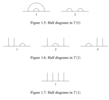
A finite indexing setT(λ)is given by Figure 1.5, Figure 1.6 and Figure 1.7.

1 2

Figure 1.5: Half diagrams inT(0)

1 2 3

Figure 1.6: Half diagrams inT(2)

1

Figure 1.7: Half diagrams inT(4)

The basis element in Figure 1.2 has been constructed by drawing the second half

dia-gram in the northern edge and the first half diadia-gram in the southern edge of the figures in

Figure 1.6. Let us construct all basis elements ofT L4(δ).

Let us name the basis elements in the formCλ

st, wheresandtare half diagrams inT(λ)

C220

C0

12 C210

C110

Figure 1.8: Basis elements ofT L4(δ)with0lines

C112 C222 C332

C2 23

C2 12

C2

32 C212

C2 31

C2 13

Figure 1.9: Basis elements ofT L4(δ)with2lines

C4 11

Figure 1.10 are the basis elements of T L4(δ). Therefore, set of basis elements of T L4(δ)

can be written as

C ={C₁₁0 , C₂₂0 , C₁₂0 , C₂₁0 ,

C₁₁2 , C₂₂2 , C₃₃2 , C₁₂2 , C₂₁2 , C₁₃2 , C₃₁2 , C₂₃2 , C₃₂2 , C₁₁4 }.

The order on the elements ofΛis as follows:

0 ≥ 2 ≥ 4.

Let us find the basis ofAˇ0_,Aˇ2_andAˇ4_.

Basis ofAˇ0 ={C_stµ :s, t ∈T(µ)andµ > 0}

=∅

Basis ofAˇ2 ={C_stµ :s, t ∈T(µ)andµ > 2} ={C₁₁0 , C₂₂0 , C₁₂0 , C₂₁0 }

Basis ofAˇ4 ={C_stµ :s, t ∈T(µ)andµ > 4} ={C₁₁0 , C₂₂0 , C₁₂0 , C₂₁0 ,

C₁₁2 , C₂₂2 , C₃₃2 , C₁₃2 , C₃₁2 , C₂₃2 , C₃₂2 , C₁₂2 , C₂₁2 }

This example helped us to understand the basis elements of algebraAand its idealAˇλ

for eachλ ∈ Λ. This understanding will help us to continue provingT Ln(δ)is a cellular

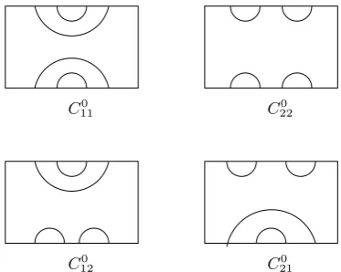
C0

21 C120

Figure 1.11: Basis to basis map

First condition: Anti-isomorphism

Define the map∗ofAas follows

∗:A→A

C_stλ∗ =C_tsλ.

This mapping reflects diagrams upside down as shown in Figure 1.11 for then = 4case.

Let us explain why∗is an anti-homomorphism. We need to show

(ma)∗ =a∗(m)∗.

The left-hand side of the above equation says find the multiplication mathen flip upside

down. On the other hand, the right-hand side says first flip a then flip m then multiply.

Obviously both are the same. From this we can say ∗ is an anti-homomorphism. ∗ is

injective by the way it is defined (it takes a basis to a basis). Now we will show ∗ is

surjective by using the rank nullity-theorem.

dim(A)=dim(Ker(∗)) +dim(Im(∗))

We know that

dim(ker(∗)) = 0.

Therefore, this implies that

t

s′

t′ s

Figure 1.12:

and so ∗is surjective. We have shown ∗ is anti-homomorphism, injective and surjective

therefore,∗is anti-isomorphism.

Second condition:

Now we will check the second condition of the cellular basis. Let Cλ

st be a basis element

of A and a ∈ A. We can write a as the linear combination of the basis elements ofA.

Therefore,acan be written as follows

a=∑dλ′s′t′Cλ ′ s′t′,

wheredλ′s′t′ ∈C. If we findCstλawe will get

C_stλa=C_stλ∑dλ′s′t′Cλ ′ s′t′

=∑dλ′s′t′CstλC

λ′ s′t′.

Figure 1.12 illustrates the multiplication ofCλ stCλ

′

s′t′. The product of these two diagrams is

a new diagram whose numberλ′′of propagating lines is less than or equal to the minimum

of the two numbersλandλ′. That is in the order onΛwe haveλ′′ ≥max(λ, λ′).

Case (i)λ=λ′.

(order onΛis not being used). First we look into the situation that multiplication gives the

same number of propagating lines. In this situation, we may get loops at the middle of the

diagrams when southern edge half diagramt of Cλ

st and northern edge half diagrams′ of Cλ′

s′t′ meet each other. If the number of propagating lines is unchanged then the

multiplica-tion does not affect the northern edge s ofCλ

st and the southern edge of Cλ ′

s′t′. Therefore,

we can say

C_stλC_sλ′′_t′ =rC_stλ′.

Hereris dependent ontands′and most importantly not dependent ons.

Now we look into the situation where multiplication gives fewer propagating lines thanλ

andλ′ (order onΛ is not being used). Let us say, we getλ′′ number of propagating lines.

According to our orderλ′′is greater thanλ. Therefore,

C_stλC_sλ′′t′ =αC λ′′ s′′t′′,

whereC_sλ′′′′_t′′is a basis element constructed from the half diagrams inT(λ′′)andα∈C. Case (ii)λ < λ′.

In this case multiplication gives us fewer propagating lines thanλ(order onΛ is not being

used). Let us say we getλ′′propagating lines. According to our order,λ′′is greater thanλ.

Therefore, this case is very similar to the latter part of Case(i). This implies that,

C_stλC_sλ′′_t′ =αC_sλ′′′′_t′′,

where Cλ′′

s′′t′′ is a basis element constructed from the half diagrams in T(λ′′), α ∈ C and λ′′ > λ.

Case (iii)λ > λ′

(order onΛis not being used). Let us say we getλ′′number of propagating lines. According

to our orderλ′′ greater than or equal toλ. Ifλ′′ =λthen

C_stλC_sλ′′_t′ =rC_stλ′.

Hereris dependent ontands′and most importantly not dependent ons.

Ifλ′′> λthen,

C_stλC_sλ′′_t′ =αC_sλ′′′′_t′′,

where C_sλ′′′′t′′ is a basis element constructed from the half diagrams in T(λ′′), α ∈ C and λ′′ > λ.

From Cases (i–iii),we see that

C_stλa =∑rC_stλ′+

∑

αC_sλ′′′′_t′′.

This can be written as

C_stλa≡∑rC_stλ′ mod ˇAλ.

Hence(C,Λ)is a cellular basis ofA. Therefore,A=T Ln(δ)is a cellular algebra.

Example 1.2.4. Let the algebraAbeT L4(δ)andλ = 2. By (1.1.3) we have that A2 is a

subalgebra ofA with basis elements of the formC_stµ,where µ ≥ λ. Similarly, by (1.1.2)

and Lemma 1.1.2(ii) we have thatAˇ2 ⊂ A2 is an ideal in A2 with basis elements of the formC_stµ, whereµ > λ. Therefore, A2/Aˇ2 is an algebra with basis elements of the form

C_st2 + ˇA2.

A2/Aˇ2 ∼=algebra with basis elements have exactly 2 propagating lines and ifais a diagram andbis a diagram anda.bhas0number of

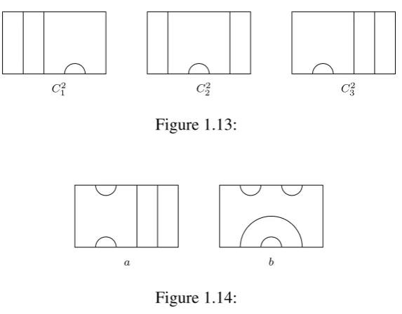
C2

1 C22 C32

Figure 1.13:

a b

Figure 1.14:

The right cell moduleC2 _{is a rightA-module with basis as in Figure 1.13. The set of basis}

elements ofC2_is

{C_t2 :t∈T(2)}={C₁2, C₂2, C₃2},

whereT(2), the set of labels with two propagating lines, is given by{1,2,3}.These three

basis elements have been constructed by fixing the northern edge half diagram and choosing

the southern edge half diagram fromT(2).

For eacha∈Awe have

C_t2a= ∑ v∈T(2)

rvCv2 mod ˇA

2_{. (1.2.2)}

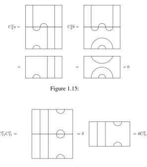
If we take algebra elementsaandbas in Figure 1.14, thenC2

2aandC22bare illustrated

in Figure 1.15. From these Figures we can say, C2

2ais C32 andC22b is0. This helps us to

understand the multiplication in (1.2.2).

We will work out the inner product⟨ , ⟩of the cell moduleC2_{basis elements in the}

= = = 0

C2

2a= C22b=

Figure 1.15:

C2

11C112 = =δ =δC112

Figure 1.16:

Example 1.2.5. Let us consider the algebra T L4(δ) and the associated cell module C2.

Figure 1.6 shows the half diagrams ofT(2). Therefore, the basis elements ofC2_are

{C₁2, C₂2, C₃2}.

By using (1.1.12) we can find the following.

i) ⟨C2

1, C12⟩C112 =C112 C112

From Figure 1.16, we can say multiplication ofC2

11andC112 gives usδC112 . From this

we can say,

C11C2 212 = = =C112

Figure 1.17:

This implies that

⟨C₁2, C₁2⟩=δ.

ii) ⟨C₁2, C₂2⟩C₁₁2 =C₁₁2 C₂₁2

From Figure 1.17, we can sayC₁₁2 C₂₁2 gives usC₁₁2 . From this we can say

⟨C₁2, C₂2⟩C₁₁2 =C₁₁2 .

Therefore,

⟨C₁2, C₂2⟩= 1.

iii) ⟨C₁2, C₃2⟩C₁₁2 =C₁₁2 C₃₁2

From Figure 1.18, we can sayC₁₁2 C₃₁2 isC₂₂0 . From this we can say

⟨C₁2, C₃2⟩C₁₁2 =C₂₂0 .

Therefore,

C11C2 312 = = =C220

Figure 1.18:

From these and similar calculations, we get

⟨C₁2, C₁2⟩=⟨C₂2, C₂2⟩=⟨C₃2, C₃2⟩=δ ⟨C₁2, C₂2⟩=⟨C₂2, C₃2⟩= 1

⟨C₁2, C₃2⟩= 0.

(1.2.3)

Example 1.2.6. Let us find radC2 _{of the cell module of the algebra T L}

4(δ). According

to (1.1.13) we can say

radC2 ={x∈C2 :⟨x, y⟩= 0for ally∈C2}.

Suppose ⟨x, y⟩ = 0 with x and y in C2_{. Therefore, we can write x and y as the linear}

combination of the basis elements ofC2. That is

x=α1C12+α2C22+α3C32,

y=β1C12+β2C22+β3C32.

Substituting for x, y and by solving ⟨x, y⟩ = 0 with the help of (1.2.3) and the

proposi-tion 1.1.4 we get

However, this equation can be written as

(α1δ+α2)β1+ (α1+α2δ+α3)β2+ (α2+α3δ)β3 = 0.

The above equation should be true for all values ofβ1,β2 andβ3. Therefore, we can say

α1δ+α2 = 0, (1.2.4)

α1+α2δ+α3 = 0, (1.2.5)

α2+α3δ = 0. (1.2.6)

Equations (1.2.4), (1.2.5) and (1.2.6) can be written as the matrix equation      

δ 1 0

1 δ 1

0 1 δ

            α1 α2 α3     

=0. (1.2.7)

We get non zero solutions to (1.2.7) only if

det      

δ 1 0

1 δ 1

0 1 δ

     = 0.

This implies

δ(δ2−2) = 0.

From this we can sayδ= 0orδ=±√2.

Ifδ̸= 0andδ ̸=±√2thenα1 =α2 =α3 = 0.Therefore,x= 0,which implies that

radC2 ={0}.

Whenδ = 0equations (1.2.4), (1.2.5) and (1.2.6) give usα2 = 0andα3 =−α1. This

implies that

radC2 ={α1(C12−C 2

3) :α1 ∈C},

which is a one dimensional space with basis (C2

1 −C32). In this case C2 is not a simple

module.

Whenδ =±√2equations (1.2.4), (1.2.5) and (1.2.6) give usα2 =∓

√

2α1 andα3 =

α1. Therefore,

radC2 ={α1(C12∓

√

2C₂2+C₃2) :α1 ∈C},

which is a one dimensional space with basis C₁2 ∓√2C₂2 +C₃2. In this case C2 is not a simple module.

We have shown thatC2is a simple module if and only ifδ ̸= 0andδ̸=±√2. Similarly we can show thatC0is a simple module if and only ifδ̸= 0andδ̸=±1andC4is a simple module for allδ ∈C.

1.3

The bubble algebra

Bubble algebras were first introduced in 2003 by Grimm and Martin [30]. These are

di-agram algebras which provide multiparameter generalizations of the Temperley-Lieb

al-gebra [60, 44]. They can be used to help solve the Yang-Baxter equation [30, section 3,

equation (5)].

In this section, we will define the bubble algebra and show that it is a cellular algebra.

Thereafter, we will discuss the cell modules of the bubble algebra and their reducibility.

Figure 4.1 denotes the labeling for the red, green and black propagating lines and arc colour

: red colour

: green colour : black colour

Figure 1.19: Colour labeling

1.3.1

Formulating the bubble algebra model with two colours

Just as for the Templerley-Lieb algebra, we shall first define a basis using diagrams, and

them introduce a multiplication rule on diagrams. The basis of this algebra will consist of

rectangular diagrams withn nodes at the northern edge andn nodes at the southern edge

which connect the nodes in pairs with two different colours red and green, without any

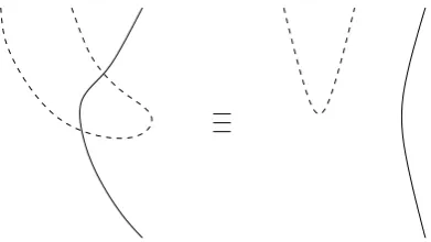
crossings of strings of the same colour and with no internal loops. Different colour strings

can cross each other, but we exclude crossing occurring on the frame of the rectangle. For

example, look at Figures 1.20 and 1.21. (These figures have been taken from [30, Section

2].)

Figure 1.20: Both are equivalent

Let us think of this, as Grimm and Martin [30] did, as lines embedded not in a rectangle,

Figure 1.21: Both are not equivalent

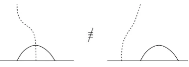
together along certain lines to trap bubbles). We allow red lines on the weld and the back

of the sheet; green lines are allowed on the welds and the front sheet.

Figure 1.22: Bubble wrap and the equivalent rectangular diagram

In this realization, lines on the same sheet(or on the weld) are not allowed to touch.

Figure 1.22 shows this and the equivalent rectangular diagram. (This figure has been taken

from [30, section 2].)

We define the multiplication of the diagrams whenever the number of end points match

up. We call the match up precise if the colours match up precisely. The composite is zero

unless the match up is precise. If the match up is precise, then we concatenate the diagrams

just as for the Temperley-Lieb algebra. When we multiply two diagrams, if we get any loop

inside then that diagram can be replaced by an appropriate loop replacement scalar times

the rest of the diagram. If the loop is red (respectively green) then the loop replacement

scalar isδR(respectivelyδG).

We denote a bubble algebra withnnodes and2colours red and green byT L2

Figure 1.23: A basis element ofT L2

3(δR, δG)

Figure 1.24: Loop form at the middle

whereδR, δGare the red and green loop replacement parameters. We can define anhcolour

generalization asT Lh

n(δC1, . . . , δCh), whereδCiis the loop replacement scalar for the colour

Ciloop for eachi∈ {1, . . . , h}.

Our modules and algebras have more than one colour. Instead of using actual colours,

we have used different types of lines to denote the label of the colours.

Example 1.3.1. Let us consider the algebraT L2

3(δR, δG). It has three nodes at the northern

and southern edges with two colours red and green. Figure 1.23 is a basis element of

T L2

3(δR, δG). Figure 1.24 is an example of the multiplication of two diagrams. This is

Figure 1.25: Loop removed

1.3.2

The bubble algebra is a cellular algebra

We will show that the bubble algebra is a cellular algebra. The full proof of this has not

previously been given. Therefore, it is quite an important matter to discuss.

Proposition 1.3.2. The bubble algebraT Lh_n(δC1, . . . , δCh)is a cellular algebra.

Proof. We consider the finite partially ordered set

Λ =

{

(c1, . . . , ch) : 0 ≤ci ≤n, 1≤i≤hand h

∑

i=1

ci =n−2tfor somet ≥0

}

.

In our diagramsciwill be the number of colourCi propagating lines andtwill denote the

total number of arcs. LettCi denote the number ofCicolour arcs. Therefore,tcan be given

by

t= h

∑

i=1

tCi.

An arc can be constructed by connecting two nodes. Therefore, the total number of

propa-gating lines will ben−2tfor some0≤t≤ n₂. Therefore, we can say

h

∑

i=1

ci =n−2t

and so each diagram is associated to an element inΛ. Define the order onΛby

Letλ ∈Λ. Therefore,λcan be given by

λ = (c1, . . . , ch)

for someci ∈ {1, . . . , n}. We define the finite indexing setT(λ)to contain half diagrams

withci colourCi propagating lines, wherei = 1,2. . . , h. (Note that there is no condition

on the colour of any arcs.) As for the Temperley-Lieb algebra, we can form a unique

bubble algebra diagram from a pair of half diagrams in T(λ) by inverting the first and

concatenating. It is clear that the set of all possible basis elements of the bubble algebra

T Lh

n(δC1, . . . , δCh)arises as we allowλto vary. Let us call the algebraAand set

C ={C_stλ :λ∈Λands, t∈T(λ)}.

HereC_stλ is the basis element ofAwiths, t ∈ T(λ), wheresis the upper half and tis the

lower half diagram of the basis element. Following (1.1.2) we set

ˇ

Aλ =span{C_stµ :µ∈Λandµ > λ} (1.3.2)

Now we define the anti-isomorphism “∗” as follows.

∗:A→A

C_stλ∗ =C_tsλ

which corresponds to reflecting a diagram in the horizontal axis.

The verification that

(ma)∗ =a∗m∗. (1.3.3)

Now we check the second condition. Let Cλ

st ∈ C and a ∈ A. An element acan be

written as a linear combination of the basis elements inA. Therefore we can giveaas

a=∑dλ′s′t′Cλ ′ s′t′,

wheredλ′s′t′ is some scalar inC. If we findCstλawe will get

C_stλa=C_stλ∑dλ′s′t′Cλ ′ s′t′

=∑dλ′s′t′CstλC

λ′ s′t′.

Now we analyze the possible values ofCλ stCλ

′ s′t′

Case (i)λ=λ′.

In this situation if the colour sequences match and the number of propagating lines does

not change then

C_stλC_sλ′′_t′ =rC_stλ′,

wherer = 1or a monomial inδC1. . . . , δCh. Thisris not dependent ons, since any loops

are not dependent ons. If the colours intands′ did not match up then the product will be

zero.

If the colour sequences match and the number of propagating lines does change, say toλ′′,

then we get less propagating lines thanλ. Therefore,λ′′ greater thanλand

C_stλC_sλ′′t′ =r′′Cλ ′′

s′′t′′ ∈Aˇλ.

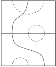
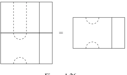
Case (ii)λ̸=λ′.

In this situation two things can happen. If the colors do not match up then

=

Figure 1.26:

On the other hand, if the colours match up let us denote byλ′′ the number of propagating

lines in the product. In this situation we get less than or equal to λ propagating lines.

Therefore, according to our order in (1.3.1) we can sayλ′′ > λorλ′′=λ.

Whenλ′′ > λwe can say

C_stλC_sλ′′_t′ =r′′C_sλ′′′′_t′′ ∈Aˇλ.

Whenλ′′=λwe have by the same argument as in case (i) that

C_stλC_sλ′′_t′ =rC_stλ′,

From case(i) and case (ii) we can say

C_stλa =∑rC_stλ′+

∑

r′′C_sλ′′′′_t′′

=∑rC_stλ′ modAˇλ

Hence we have shown that(C,Λ)is a cellular basis ofA, and soA=T Lh

n(δ1, . . . , δh)is a

cellular algebra.

Example 1.3.3. From the above proof we know thatT L2

3(δR, δG)is a cellular algebra. We

λ Half diagrams inT(λ) (3,0) Figure 1.27

(0,3) Figure 1.28

(2,1) Figure 1.29

(1,2) Figure 1.30

(1,0) Figure 1.31

(0,1) Figure 1.32

Table 1.1:

Let Λhave elements as ordered pairs with first part denoting the number of red

prop-agating lines and second part denoting the number of green propprop-agating lines. If we take

any half-diagram in a diagram inT L2

3, it can either have all propagating lines or one

prop-agating line and one arc. If we takeλ∈Λit will be of the form

λ= (m, n),

wheremdenotes the number of red propagating lines andn denotes the number of green

propagating lines. Therefore, we can say

m+n = 3or1.

From this we can say

Λ ={(3,0),(2,1),(1,0),(0,3),(1,2),(0,1)}.

For eachλ∈Λthe indexing setT(λ)gives half diagrams withmbeing the number of red

propagating lines andnbeing the number of green propagating lines. Let us find the half

diagrams for each value ofλ. We illustrate these in the Figures indicated in Table 1.1.

The order inΛis

(a, b)≥(c, d)if and only ifa≤candb ≤d.

1

Figure 1.27: Half diagram inT((3,0))

1

Figure 1.28: Half diagram inT((0,3))

1 2 3

Figure 1.29: Half diagrams inT((2,1))

1 2 3

Figure 1.30: Half diagrams inT((1,2))

1 2 3

4 5

1 2 3

4 5

Figure 1.32: Half diagrams inT((0,1))

(0,1)

(1,2) (0,3)

(1,0)

(3,0) (2,1)

Figure 1.34: Basis element ofT L2

3(δR, δG)

In general this order is very important to showT L2

3 is a cellular algebra even though it

is not important in this example.

Let us pick the half diagrams denoted by1and4fromT((1,0)). Draw the half diagram

1at the northern edge and 4at the southern edge of the rectangular box. We will get the

diagram in Figure 1.34. This is a basis element ofT L2

3(δR, δG). We name thisC

(1,0) 14 .

Example 1.3.4. Let algebraAbeT L2

3(δR, δG). We find the basis elements ofC

(1,0) 3 . This

is anA-submodule ofA(2,1)_/Aˇ(2,1)_{. Half diagrams inT((1,0)) are in Figure 1.31.}

There-+ _Aˇ(1,0)

ˇ

A(1,0)

+

ˇ

A(1,0)

+

+ _Aˇ(1,0)

+ _Aˇ(1,0)

Figure 1.35:

c(1,0)1 c (1,0)

2 c

(1,0) 3

c(1,0)4 c

(1,0) 5

Figure 1.36:

Figure 1.35. (We normally ignore the final term Aˇ(1,0).) If we look at each diagram, all have the same northern edge half diagram.

Basis elements of the cell moduleC(1,0)_areC(1,0) 1 ,C

(1,0) 2 ,C

(1,0) 3 ,C

(1,0) 4 andC

(1,0) 5 which

are in Figure 1.36.

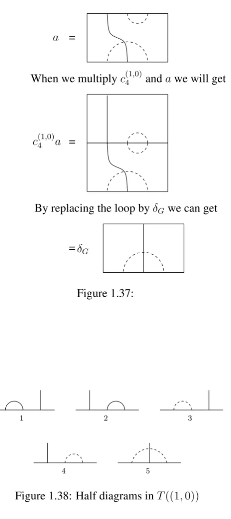
Let see what will happen if we multiplyC₄(1,0) in Figure 1.36 by the algebra elementa

fromT L2

3 which is illustrated in the Figure 1.37. From this we can say

C₄(1,0)a=δGc

(1,0) 5 .

Example 1.3.5. Let algebra Abe T L2

3(δR, δG)and consider the cell moduleC(1,0). Now

we find the inner product between the basis elements of the cell module. Figure 1.38 shows

the half diagrams of the basis element of the cell moduleC(1,0)_{. Basis ofC}(1,0) _{is given by}

C(1,0) ={C₁(1,0), C₂(1,0), C₃(1,0), C₄(1,0), C₅(1,0)}.

Let us apply the rule

=

a

=

c(1₄,0)a

=δG

When we multiplyc(1₄,0) andawe will get

By replacing the loop byδGwe can get

Figure 1.37:

1 2 3

4 5

in (1.1.12) All the changes happen at the middle of the two diagrams. Half diagrams

correspond to the basis in< , >responsible for those changes. This observation makes the

working out< , >very easy.

< C₁(1,0), C₄(1,0) >= 0 < C₃(1,0), C₃(1,0) >=δG < C₁(1,0), C₅(1,0) >= 0 < C₃(1,0), C₄(1,0) >= 0 < C₂(1,0), C₂(1,0) >=δR < C₃(1,0), C₅(1,0) >= 0 < C₂(1,0), C₃(1,0) >= 0 < C₄(1,0), C₄(1,0) >=δG < C₂(1,0), C₄(1,0) >= 0 < C₄(1,0), C₅(1,0) >= 0 < C₂(1,0), C₅(1,0) >= 0 < C₅(1,0), C₅(1,0) >=δG

Example 1.3.6. Let us find radC(1,0)

radC(1,0) ={x∈C(1,0) :< x, y >= 0for ally∈C(1,0) }.

Letxandybe elements inC(1,0)_{. Therefore, we can writexandyas linear combinations}

of the basis elements ofC(1,0)_{. That is}

x=α1C (1,0)

1 +α2C (1,0)

2 +α3C (1,0)

3 +α4C (1,0)

4 +α5C (1,0) 5 ,

y=β1C (1,0)

1 +β2C (1,0)

2 +β3C (1,0)

3 +β4C (1,0)

4 +β5C (1,0) 5 .

Suppose< x, y >= 0for ally. By substituting forxandywe obtain the following.

α1δR+α2 = 0 (1.3.4)

α1+α2δR= 0 (1.3.5)

α3δG = 0 (1.3.6)

α4δG = 0 (1.3.7)

If we solve (1.3.4) and (1.3.5) we obtain

α1(δR2 −1) = 0. (1.3.9)

When δR ̸= ±1 and δG ̸= 0 then equations (1.3.4), (1.3.5), (1.3.6), (1.3.7), (1.3.8)

and (1.3.9) imply

α1 =α2 =α3 =α4 =α5 = 0.

Therefore,

radC(1,0) ={0}.

From this we can sayC(1,0)_{is a simple module for almost every value ofδ.}

WhenδR =±1andδG̸= 0we have

radC(1,0) ={α1(C1(1,0) ∓C (1,0)

2 )|α1 ∈C}.

This is a one dimensional vector space with basisC₁(1,0)∓C₂(1,0). WhenδR ̸=±1andδG= 0we have

radC(1,0) ={α3C (1,0)

3 +α4C (1,0)

4 +α5C (1,0)

5 |α3, α4, α5 ∈C}.

This is a three dimensional vector space with basisC₃(1,0),C₄(1,0) andC₅(1,0). WhenδR =±1andδG= 0we have

radC(1,0) ={α1(C (1,0) 1 ∓C

(1,0)

2 ) +α3C (1,0)

3 +α4C (1,0)

4 +α5C (1,0)

5 |α1, α3, α4, α5 ∈C}.

This is a four dimensional vector space with basisC₁(1,0) ∓C₂(1,0), C₃(1,0), C₄(1,0)andC₅(1,0).

The moduleC(1,0) is not a simple module in the last three cases.

If we repeat this calculation for C(0,1)_{, C}(2,1)_{, C}(1,2)_{, C}(3,0) _{and C}(0,3) _{we obtain the}

C(1,0)_{is a simple module ifδ}

R̸=±1andδG ̸= 0. C(0,1)_{is a simple module ifδ}

G ̸=±1andδR̸= 0.

C(2,1)_{, C}(1,2)_{, C}(3,0)_andC(0,3) _{are simple modules for allδ}

Chapter 2

Towers of recollement

In this chapter we are going to discuss an axiomatic framework for studying the

representa-tion theory of towers of algebras. This has been introduced by Cox, Martin, Parker and Xi

[13] in 2006. They introduced a new class of algebras called contour algebras, and proved

that they satisfy the axiomatic framework of towers of recollement. Brauer and walled

Brauer algebras also form towers of recollement [10].

Let An (with n ∈ N) be a family of finite dimensional algebras, with idempotents en in An, defined over an algebraically closed fieldK. Such a family of algebras which

satisfies the axioms(A1)to(A6)which we are going to discuss soon is called a tower of

recollement.

If a family of algebras is a tower of recollement, then we can apply Theorem 2.1.27

which we are going to discuss later in this chapter. This Theorem helps us to know whether

we have a non-zero homomorphism between two standard modules by reducing to the case

2.1

Bubble algebras satisfies the axiomatic framework

We are going to show that our family of algebrasT Lh

n(withn ∈ N) is a tower of

recolle-ment when all of theδCi are non-zero. We introduce each axiom for a tower of recollement

followed by the proof that the bubble algebra satisfies it.

In chapters 4 and 6, we will discuss how to find the non-zero homomorphisms (if they

exist) between two given cell modules where the first has no arcs. If we consider two

modules with the first having some arcs, then by using the Theorem 2.1.27, we can reduce

the size of the modules until the first module has no arcs in it. Therefore, it is enough to

consider whether a homomorphism between the given two modules exists or not in this

special case.

LetAn = T Lhn(δC1, . . . , δCh). We want to define idempotentsen inAn. Leten be the

sum over all possible colourings of strings and arcs (with the two arcs coloured the same)

of diagrams as in Figure 2.1, where each such diagram is multiplied by the scalar_δ1

Ci which corresponds to the colour of the arc at the northern edge and southern edge of the diagram.

As the arcs at the northern edge and southern edge of the diagram are the same in colour

they can be coloured inhways, and the rest of then−2lines can each be coloured by h

different colours. Therefore,enis a sum ofhn−1diagrams. To be an idempotent elementenshould satisfy the condition

e2_n =en.

When we finden×en, we get zero for the southern edge colour sequence of the diagrams

comes from the firsten, and the northern edge colour sequence of the diagram come from

the second en do not match. However, we get a loop at the middle of the diagram if the

edge colour sequence of the diagram coming from the second en are the same. For this

reason we defineden as the sum of diagrams as in Figure 2.1 multiplied by the scalar _δ1

Ci, as this gives the desired idempotent property.

. . .

Figure 2.1:

We will show our algebrasAn = T Lhn satisfies the tower of recollement axioms (A1)

to (A6) in [13].

Definition 2.1.1. LetΛn be an indexing set for the simple An-modules and Λn be an

in-dexing set for the simpleAn/AnenAn-modules.

For any algebraAwith idempotente∈Awe have the following Theorem.

Theorem 2.1.2. (Green [22]) Let{L(λ) : λ ∈ Λ}be a full set of simpleA-modules, and

setΛe_{={λ∈Λ :L(λ)e̸= 0}. Then{L(λ)e:λ∈Λ}e_{}is a full set of simpleeAe-modules.}

Further, the simple modulesL(λ)withλ∈Λ\Λe_{are a full set of simpleA/AeA-modules.}

If we take the algebraAto beAn, the indexing setΛto beΛnand the idempotenteto

beenin this Theorem, thenΛeisΛn−2andΛnisΛn\Λn−2.

Axiom 2.1.3. (A1) For eachn≥2we have an isomorphism