Modeling and control design of a Vienna rectifier based electrolyzer

Modeling and Control Design of a Vienna

Rectifier Based Electrolyzer

Jos´e Luis Monroy-Morales, M´aximo Hern´andez- ´

Angeles

Instituto Tecnol´ogico de Morelia Morelia, Michoac´an M´exico Email: jlmonroy [email protected],

mhernand [email protected]

David Campos-Gaona, Rafael Pe˜na-Alzola,

Martin Ordonez, Walter M´erida

Department of Electrical and Computer Engineering The University of British Columbia

2332 Main Mall. Vancouver, BC Canada V6T 1Z4l Email: [email protected], [email protected],

[email protected], [email protected]

Abstract—Hydrogen production is an interesting alternative of storing energy. Electrolyzers produce hydrogen through water electrolysis; the resulting hydrogen is later used to generate electricity by using fuel cells, that reverse the process. Electrolyzers use rectifiers to convert the gridacvoltage intodc

voltage for supplying the electrolyzer cells. Previous research used a rectification process based on conventional rectifiers (diode- or thyristor-based) which draw non-sinusoidal current from the main grid. This requires increased filtering to prevent power quality problems and equipment malfunctioning/failure. In addition, previous literature assumed simplified models for the power electronics converters and lacked a detailed control system. The Vienna rectifier is a non-regenerative converter that produces sinusoidal currents with low losses due to the reduced number of active switches. This manuscript proposes using the Vienna rectifier as an interface to connect electrolyz-ers to theacgrid. Thedcvoltage applied to the electrolyzer is regulated by using another dc-dc converter, which is selected to be a synchronous buck converter for simplicity and maximum efficiency. In this paper, the models of the Vienna rectifier, synchronous buck converter, and the electrolyzer are developed along with their respective controls. The control system has the ability to function in two operation modes for the overall reference: hydrogen production and power demand. The first one is adequate for grid-connected operation and the later for off-grid operation. Simulation results are given to show the validity of the proposed procedures.

Index Terms—Alkaline electrolyzer, vienna rectifier, hydro-gen storage, fuel cell, hydrohydro-gen production, water electrolysis.

I. INTRODUCTION

The awareness in environmental pollution requires finding alternate ways to produce energy with low greenhouse gas emissions. There are various ways to store renewable energy. Battery banks can be a solution of energy storage, but they have medium energy density, self-discharge and leakage characteristics. They are also not suitable for long-term energy storage. Pumped hydro and compressed air energy storages are low cost options, but they have lower efficiencies and mostly dependent on the geographical location. Hydrogen is more suitable for long-term load leveling applications and fuel cells and electrolyzers can have a vital role in distributed energy generation and storage with minimal emissions [1, 2]. Hydrogen is often referred to as the energy carrier of the future as it can be used to store

intermittent renewable energy. Hydrogen can be produced from electrical power and water by using an electrolyzer. An electrolyzer is a device that converts electricity into chemical energy to produces hydrogen through the process of electrolysis [3–6]. Fuel cells can be used to return the energy to the grid or to an electric vehicle with no emissions, high efficiency and fast response. Fuel cells also have the capability to supply electricity for unlimited time as long as the required amount of hydrogen is present in the deposit.

An increase in energy demand and decrease in fossil fuels leads to the need to find alternate ways to produce energy with low greenhouse gas emissions. In consequence, there is a great need for accelerating the development and implementation of new technologies for alternative energies [7]. Electrolyzers use rectifiers to convert the gridacvoltage intodcvoltage for supplying the electrolyzer cells. Previous research used a rectification process based on conventional rectifiers (diode- or thyristor-based) which draw non-sinusoidal current from the main grid. This requires increased filtering to prevent power quality problems and equipment malfunctioning/failure due to electromagnetic interference (EMI). In addition, previous literature assumed simplified models for the power electronics converters and lacked a detailed control system. The Vienna rectifier is one of the most popular topologies for three-phase power factor correction due to its good performance and relatively low costs [8–10]. The Vienna rectifier is a non-regenerative converter that produces sinusoidal currents with unity power factor and low losses due to the reduced number of active switches.

L ie

v_DC

Vienna Rectifier Synchronous Buck Converter

G

Grid _i

A B C

A

+

L_e

N

2C_DC v_DCu

+

v_DCl

+ 1

2 3

1 Grid-side Converter: Vienna Rectifier

2 Available DC-link for Auxiliary Services

3 Synchronous Buck Converter for Electrolyzer

H₂

Electrolyzer

e_g v ve

v_b

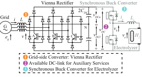
Fig. 1. Overall representation of the proposed system. thus increasing efficiency [11]. In this paper, the models of the Vienna rectifier, synchronous buck converter, and the electrolyzer are developed along with their respective controls. The control system has the ability to function in two operation modes for the overall reference: hydrogen production and power demand. The first one is adequate for grid-connected operation and the later for off-grid operation. Fig. 1 shows the overall representation of the proposed new application. The Vienna rectifier has sinusoidal voltage and current in phase inputs and unity power factor and the synchronous buck converters control the amount of produced hydrogen/power. Simulation results are given to show the validity of the proposed procedures.

II. CONTROL OF THEASSOCIATEDPOWERELECTRONICS Rectifiers are needed in electrolyzer systems to transform the grid acvoltage to dcvoltage. The output voltage of the fuel cell array varies significantly with the hydrogen supply rate and the pressure. Therefore, adc−dcconverter is also required to control the electrolyzer system.

A. Vienna Rectifier Control

When using carrier-based pulse width modulation (PWM) and unity power factor the control of the Vienna rectifier is very similar to that of the full-bridge converter. The control employs a rotating reference frame synchronized with theac -grid voltage vector by using a phase-locked loop (P LL). The voltages and currents occur as constant vectors in the d−q reference frame in steady state. Considering the converter system connected to grid, the phase voltages and currents are given by the equation,

vabc=Riabc+L

diabc

dt +Vabc,conv (1)

where vabc, iabc, vabc,conv are ac voltages, currents and

converter input voltages respectively. R and L are the resistance and filter inductance between the converter and the ac system. Assuming perfect synchronization with the grid voltage, the voltage equations in d−q synchronous reference frame are:

vd=Rid+L

did

dt −ωgLiq+vdconv (2)

vq =Riq+L

diq

dt +ωgLid+vqconv (3)

The subscript d and q stand for direct and quadrature respectively. In this configuration, the active and reactive power are controlled by theid andiq currents respectively.

The control system is based on nested loops with fast inner current control loops and slower outer dc voltage control loop. The current reference for iq is set to zero for unity

power factor.

Similarly on the output side,

Idc=C

dVdc

dt +IL (4)

The power balance relationship between theacinput anddc output is given as,

P =3

2(vdid+vqiq) =VdcIdc (5) where Vdc and Idc are dc output voltage and current

respectively.

The grid voltage vector is defined to be along thed−axis direction, and then a virtual grid flux vector can be assumed to be acting along theq−axis. With this alignment,vq = 0

and the instantaneous real and reactive power injected into or absorbed fromac system is given by,

p= 3

2vdid (6)

q=−3

2vdiq (7)

Hence, the transformation into rotating d−q coordinate system oriented with respect to the grid voltage vector, leads to a split of the mains current into two parts. One part determines the contribution which gives required power flow into the dcbus while the other part defines the reactive power condition. The equations (6) and (7) show directly the possibility to control two current components independently. The overall scheme is shown in Fig. 2.

DC-Voltage Measurement

DC Voltage Controller (Outer Control

Loop)

Current Controller

(Inner Control Loop)

abc to dq

Transformation

AC Current Measurement

PLL

Measurement

PWM

Generator

Vienna Rectifier

i_abc

iq=0 vDC

id ref

ref

vDC ref

D_d

Dq

i_dq

Fig. 2. Overall scheme of vectorial Vienna rectifier control. The inner current control block is represented by the general block diagram shown in Figure 3.

V’_conv V_conv I I_ref

-+ PI Controller

PWM Converter

System Transfer Function

Fig. 3. General Block Diagram of Inner Current Control. is discussed below.

The equation of the P I regulator is:

R(s) =Kp+

Ki

s =Kp

_{1 +T}

is

Tis

(8)

thus for PI controller block,

{Iref(s)−I(s)}

Kp+

Ki

s

=V_conv0 (s) (9)

the converter is considered as an ideal power transformer with a time delay. The output voltage of the converter is assumed to follow a voltage reference signal with an average time delay equals half of a switching cycle, due to converter switches. Hence, the general expression is:

Y(s) = 1 1 +Tas

(10)

whereTa=Tswitch/2. Thus, for converter block,

V_conv0 (s)

₁

1 +Tas

=Vconv(s) (11)

The system behavior is governed by equations (2) and (3). As seen from the equations, the model of the converter in the synchronous reference frame is a multiple-input multiple output, strongly coupled nonlinear system. And it is difficult to realize the exact decoupled control with general linear control strategies. The transformed voltage equations of each axis have speed/frequency induced term, wgLid and

wgLiq, that gives cross-coupling between the two axes.

For each axis, the cross-coupling term can be considered as disturbance from control point of view. Thus, a dual-close-loop direct current controller with decoupled current compensation and voltage feed-forward compensation is required to obtain a good control performance. The equations (2) and (3) are rewritten as follows,

Vd−Vdconv=L

did

dt +Rid−wgLiq (12)

Vq−Vqconv =L

diq

dt +Riq−wgLid (13)

Using separate inner loop current controllers for id and iq,

give the output of voltage reference signals for two axes, which fed to the converter gives two references for the system, that are d−q components of Vconv(s): Vdconv

and Vqconv. Using Equation (9) and Equation (11), these

references are,

Vdconv= (idref−id)

Kp+

Ki

s

₁

1 +sTa

(14)

Vqconv = (iqref−iq)

Kp+

Ki

s

₁

1 +sTa

(15)

As seen from equations (12) and (13), the dandq compo-nents of the converter voltages are cross coupled. Hence, the reference used as input to system can be split in two com-ponents, one of which is obtained from converter whereas the other is a feed-forward term to eliminate the cross-coupling. With the compensation terms used for decoupling, the system input from converter is defined as

V0dconv=−(idref−id)

Kp+

Ki

s

+wgLiq+Vd (16)

V0qconv=−(iqref−iq)

Kp+

Ki

s

−wgLid+Vq (17)

Equations (16) and (17) when substituted in Eqn.(11) and equated to system equations (12) and (13) respectively, it gives,

Ldid

dt +Rid =Vdconv (18)

Ldiq

dt +Riq=Vqconv (19)

The cross coupling terms are thus cancelled out and independent control in d and q axis is achieved, which is one of the important features of vector control. Thus, current controllers of each axis operate independently. Figure 4 show the reduced diagram indandq axes.

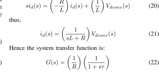
As seen from equations (18) and (19) the equations in d andq axis have a similar form. For this reason only the d-axis equations are used for further analysis. Consequently the other controller will also have the same parameters. By Laplace transformation the equation becomes:

sid(s) =

−R

L

id(s) +

1

L

Vdconv(s) (20)

thus,

id(s) =

₁

sL+R

Vdconv(s) (21)

Hence the system transfer function is:

G(s) =

₁

R

1 1 +sτ

(22)

Where the time constant of the line is defined as τ=L/R.

I_d _I_q

-+

Ti .s

Kp

(

(

1+T_a.s

(

(

1+t.s

(

(

Fig. 4. Reduced block diagram indandqaxes.

response. From (22) it can be seen that the open-loop current system has a stable pole at −R/L . This pole can be cancelled with the zero provided by the P I controller, whereKpandKiare the proportional and integral constants

of the P I current controller. Thus, choosing Ki/Kp=R/L

and Kp/L = 1/τ where τ is the time constant of the

closed-loop system. Hence the tuning of current controller by modulus optimum criteria can be summed up as,

Kp=

τ R

2T a (23)

Ki=R/τ (24)

whereτ=Ti.

Dimensioning of the dc link voltage controller is deter-mined by the transfer function between the current reference value to be given and the dc link voltage. The general diagram for the external controller is shown in Figure 5. The diagram consists of a P I controller, the inner current controller and the power transfer function of the output element system.

I_{dref Inner Current} I_d V_dc Controller

V_dcref

-+ PI Controller

System Transfer Function

Fig. 5. General Block Diagram of OuterdcVoltage Control. The equation forP I voltage controller is:

R(s) =Kpv+

Kiv

s =Kpv

1 +Tivs

Tivs

(25)

where the subscript v denotes the voltage regulator. The controller parametersKpv and Tiv = Kpv/Kiv need to be

designed for an optimum performance. For the PI controller block for outer voltage control,

{Vdcref(s)−Vdc(s)}

Kpv+

Kiv

s

=idref(s) (26)

The closed current loop gives the relation between idref

andid in the block diagram as in Fig. 4. The second order

transfer function of the inner current controller, can be approximated as:

W(s) = 1

Teqs+ 1

(27)

whereTeq=2Ta.

From the equation (5), to obtain the transfer function of the converter, third block of Figure 5, and having the condition Vq = 0, the relationship between id andIdc is:

Idc=

3 2

Vd

Vdc

id (28)

This defines the value of the current gain to be used from dc current to input current or viceversa. Substituting this value in Eqn. (4), we get,

CdVdc dt =

₃

2

Vd

Vdc

(id)−IL (29)

It is possible to observe that the dc-link current equation is a nonlinear equation. For analyzing the stability of a non-linear system in the neighborhood of a steady state operating point, it is necessary to linearize the system model around the operating point and perform linear stability analysis. The reference point for linearization is found by specifying reference input, Vdcref for the nonlinear model.

Consequently the linear expression becomes,

Cd∆Vdc dt =

₃

2

Vd,0

Vdc,ref

∆id (30)

(31)

By Laplace transformation it is:

∆Vdc(s)

∆id(s)

=

₃

2

Vd,0

Vdc,ref

1

sC

(32)

Thedclink voltage controller controls the capacitor current so as to maintain the power balance. Hence under balanced conditions,Ic= 0. That is,Idc=IL.

Thus, the reference value ofid should be,

id=

₂

3

Vdc

Vd

Idc (33)

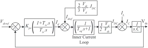
which is the feed-forward term, ensuring exact compensation for load variation. The overall control block diagram of the dc voltage controller based on Eqn. (26)-(33) is as shown in Fig. 6.

Inner Current Loop

Vdcref Vdc

-+ +- _T +

-eq.s+1

(

(

2. VV_dcd

1 s.C

I_d I_DC IC

IL

I_dref

2 3.

V_dc V_d .IDC

(

Tiv.s

Kpv

(

1+T_iv.s

In cascade control, generally the inner loop is tuned according to modulus optimum condition because of fast response and simplicity whereas the outer loop according to symmetrical optimum condition for optimizing system behavior with respect to disturbance signals. From the system block diagram as developed in Fig.6, the open loop transfer function of the system without considering the feed-forward and the disturbance input is given by,

GV,OL(s) =Kpv

_{1 +T}

ivs

Tivs

₁

Teqs+ 1

_V

dwbC

Vdcs

(34)

The open loop transfer function consists of double pole at origin. The system cannot be designed by cancelling the pole and zero, because it will result in two poles at origin and the system becomes unstable. Hence the design is chosen by using symmetrical optimum design criteria. Symmetrical Optimum method obtains a controller that forces the frequency response from a reference point to output as close as possible to that for low frequencies. The method has the advantage of maximizing the phase margin. As phase margin is maximized for given frequency, the system can withstand more delay, which is important for systems having delays. This method optimizes the control system behaviour with respect to disturbance input [12].

Eqn. (34) can be simplified by introducing K=Vd/Vdc,

andTc= 1/wb.C as follows,

GV,OL(s) =Kpv

_{1 +T}

ivs

Tivs

K Teqs+ 1

1

Tcs

(35)

wherewb= 2πf, is the base frequency.

According to the tuning criteria derived, the parameters for tuning the outer controller by symmetrical optimum are,

Tiv =a2Teq (36)

Kpv=

Tc

aKTeq

(37)

whereTeq = 2Ta andTa= Tswitch₂ =_2fswitch1 .

The inner control time response is selected in 1ms, hence, the outer control is selected 10 times this value in order to get a good performance of the controller.

B. Synchronous Buck Converter Control

In the synchronous buck converters, the lower diode is replaced by a power MOSFET with lower on-voltage drop than the forward drop of the rectifier, thus increasing efficiency. The output voltage of the synchronous buck

converterVb is set by the duty cycleD:

Vb= (D)(Vdc) (38)

with Vdc the overall dc-link voltage assumed for constant

for control. A simple analysis of buck converter circuit shown in Fig. 1 results in the following equation:

(D)(Vdc)−Ve=Le

die

dt +Reie (39)

where ie and Ve is the electrolyzer current and voltage

respectively.Leis an connection inductor to the electrolyzer

andRe is parasitic resistance. Applying Laplace transform

to (39) and rearranging, it follows:

ie(s)

(Ds)Vdc

= 1

Les+Re

(40)

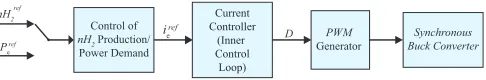
Using the transfer function from equation (40) the buck converter current is controlled in a closed loop as shown in Fig. 7. Assuming the overalldc-link voltage is constant, the consumed power is proportional to the electrolyzer current ie. Additionally, it is shown in the next section that the

hydrogen productions is also proportional to the electrolyzer current.

Current Controller

(Inner Control Loop)

PWM

Generator

Synchronous Buck Converter Pe

i_eref nH₂ref

D ref

Control of

nH₂Production/ Power Demand

Fig. 7. Scheme control of synchronous buck converter output current.

III. ELECTROCHEMICALMODEL OFELECTROLYZERS The most economically appropriate for an energy storage system are the alkaline water electrolyzers. The decomposition of water into hydrogen and oxygen can be achieved by passing a dc electricity current between two electrodes separated by a aqueous potassium hydroxide (KOH) electrolyte with good ionic conductivity [13].

I-U Characteristic Curve: The kinetic properties around the electrodes in an electrolyzer cell can be modeled based on empirical data of different proposed I −V curves. A representative plot of the theoretical and actual voltages for an alkaline water electrolyzer versus the current density at high and low operating temperatures is shown in Fig. 8. The basic relationship between current and cell voltage in a given temperature is:

V =Vrev+

I

Ar+slog

I At+ 1

(41)

Current (mA)

0 200 400 600 800 1000 1200

Ce

ll

V

ol

ta

ge

(V

)

1.2 1.4 1.6 1.8 2 2.2 2.4

= V_{ref 10º}= 1.2772 V V_{ref 80º} 1.2275 V

30º 10º

20º

40º 50º 60º_{70º 80º} 90º

100º Temperature:

Overvoltage

Fig. 8. Typical I-V curves for an electrolyzer cell at high and low temperatures.

coefficients on electrodes andVrevis the reversible voltage.

The thermodynamics of the electrochemical reactions is an important factor to be taken into account. The changes in enthalpy and entropy of the water splitting reaction induce changes in Gibb’s energy and consequently in the Vrev.

These parameters are directly affected by the working con-ditions of the Alkaline Electrolyzer. The reversible voltage can be expressed as:

Vrev=

∆G

zF (42)

where ∆G is Gibb’s energy, z is the number of electrons transferred in each reaction, here it is 2, andFis the Faraday constant. In standard condition,25◦C and1bar, the change of Gibb’s energy of water splitting is ∆G◦ = 237kJ/mol. In order to relate the ohmic resistance parameterrand over voltage coefficient t, the equation (41) can be modified in more detailed way as:

V =Vrev+

I

A(r1+r2T)

+slog[I

A(t1+ t2

T + t3

T2 + 1)]

(43)

whereT is the electrolyte temperature.

Hydrogen Production:Faraday efficiency is the proportion of the actual and theoretical hydrogen production in the electrolyzer [14]. One of the parameters that control the hydrogen production is current, so another name of Faraday efficiency iscurrent efficiency. It can be noted that parasitic current increases with the decrement of current density and the increment of temperature resulting the reduction of Faraday efficiency. This phenomenon can be expressed as:

nF =

(I A)

2

f1+ (_AI)2

∗f2 (44)

where f1 and f2 are the parameters related to Faraday efficiency.

Normally a number of electrolyzer cells are connected in

series in a stack and some stacks are connected in parallel. The number of such electrolyzer cells has an impact on the total hydrogen production [15]. The production rate is

n_H2 =nF

ncI

zF (45)

wherenc is the number of electrolyzer cells per stack.

The total amount of energy needed in water electrolysis is equivalent to the change in enthalpy ∆H. The standard enthalpy for splitting water is ∆H◦ = 286 kJ mol−1. The total energy demand∆H is related to the thermoneutral cell voltage by the expression

Vtn=

∆H

zF (46)

The energy efficiency can be calculated from the thermo neutral voltage and the cell voltage by the expression

ne=

Vtn

V (47)

The electrical inefficiencies result the unwanted heat generation in the electrolyzer which has an indirect influence on Faraday efficiency.

IV. SIMULATIONRESULTS

Simulations were conducted in order to verify the performance of the system shown in Fig. 1 along with its control strategy. The hydrogen production operative mode is used when a fixed amount of hydrogen is required, up to the maximum attainable limit of hydrogen production. This operation mode is adequate when the system is connected to the main grid. Fig. 9 shows the current and voltage waveform of phase a in pu when a step change from 0.5 to 0.8 pu in the hydrogen production reference signal is applied (hydrogen production mode).

0 0.05 0.1 0.15 0.2

-2 -1 0 1 2

time

pu

Current Voltage

Fig. 9. Hydrogen production operating mode, voltage and current of phase

ainpuwith a change from 0.5 to 0.8 in the reference signal.

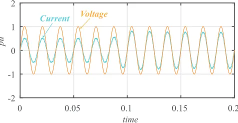
demand side management or off-grid configuration. Fig. 10 shows the current and voltage waveform of phase a in pu when a step change from 0.5 to 0.8 pu in the power demand reference signal is applied (power demand mode).

0 0.05 0.1 0.15 0.2 0.25 0.3

-2 -1 0 1 2

time

pu

Voltage

Current

Fig. 10. Power demand operating mode, voltage and current of phaseain

puwith a change from 0.5 to 0.8 in the reference signal.

In both cases, Figs. 9 and 10, the current waveform changes accordingly while remaining in phase with the ac voltage (unity power factor).

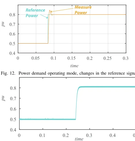
Fig. 11 shows the performance of the hydrogen production operative mode when the hydrogen production reference signal is changed from 0.5 to 0.8 pu. As seen Fig. 11 the controller tracks hydrogen production reference signal in a fast and stable manner. Fig. 12 shows the performance of the power reference operative mode when the excess of power production in theacgrid changes from 0.5 to 0.8 pu. As seen in Fig. 12 the controller drives the Vienna rectifier to absorb 0.8 of power in a fast and stable manner.

0 0.05 0.1 0.15 0.2

0.4 0.5 0.6 0.7 0.8

time

pu

n_H2 Reference

n_H2 Measure

Fig. 11. Hydrogen production operating mode, changes in the reference signal.

Figs. 13 and 14 show the change of current in the synchronous buck converter when a reference change is applied in hydrogen production mode and power reference mode respectively. The slower response of the hydrogen production mode is because of the larger time constant of the electrochemical process. This simulation results corrob-orate the proper functioning of the Vienna rectifier and the electrolyzer control modes.

0 0.05 0.1 0.15 0.2 0.25 0.3 0.4

0.5 0.6 0.7 0.8

time

pu

Reference Power

Measure Power

Fig. 12. Power demand operating mode, changes in the reference signal.

0 0.1 0.2 0.3 0.4 0.5

0.4 0.5 0.6 0.7 0.8

time

pu

Fig. 13. Hydrogen production operating mode, change in the Synchronous Buck converter current.

0 0.1 0.2 0.3 0.4 0.5 0.6

0.4 0.6 0.8

time

pu

Fig. 14. Power demand operating mode, change in the Synchronous Buck converter current.

V. CONCLUSION

The complete model of the Vienna rectifier, the synchronous buck and the electrical to hydrogen production process was developed along with the different controls. The whole system is able to characterize the relation among the different physical quantities to determine the control action that ensures the proper operation of the electrolyzer. Additionally, the electricity-to-hydrogen conversion process is carried out efficiently (because of the Vienna rectifier topology), with sinusoidal current and unity power factor in the AC mains. The proposed system operates in two modes; hydrogen production and power demand operating mode. The ability to select between these two operative modes is highly beneficial for electrical grids connected to intermittent power sources and/or requiring capability for demand side management. Simulation results corroborate the proper functioning of the proposed new application using the Vienna rectifier for the electrolyzer system.

REFERENCES

fuzzy logic controller,” in Green Computing Communication and Electrical Engineering (ICGCCEE), 2014 International Conference on, March 2014, pp. 1–6.

[2] M. Kolhe and O. Atlam, “Empirical electrical modeling for a proton exchange membrane electrolyzer,” inApplied Superconductivity and Electromagnetic Devices (ASEMD), 2011 International Conference on, Dec 2011, pp. 131–134.

[3] R. Takahashi, H. Kinoshita, T. Murata, J. Tamura, M. Sugimasa, A. Komura, M. Futami, M. Ichinose, and K. Ide, “Output power smoothing and hydrogen production by using variable speed wind generators,” Industrial Electronics, IEEE Transactions on, vol. 57, no. 2, pp. 485–493, Feb 2010.

[4] O. Bendakha and S. Larbi, “Hydrogen production system analysis us-ing direct photo-electrolysis process in algeria,” inRenewable Energy Research and Applications (ICRERA), 2013 International Conference on, Oct 2013, pp. 1123–1128.

[5] I. S.J. Anand and V. Bale, “Exergetic assessment of solar hydrogen production methods,,” Int. J. Hydrogen Energy. vol.35, pp.4901-8, 2010.

[6] W. S.-Y. X. Lan and L. You-Rong, “Advances in solar hydrogen production via two-step water-splitting thermochemical cycles based on metal redox reactions,”Renew Energ, vol. 41, pp. 1-12, 2012. [7] H. Teymour, D. Sutanto, K. Muttaqi, and P. Ciufo, “Solar pv and

battery storage integration using a new configuration of a three-level npc inverter with advanced control strategy,”Energy Conversion, IEEE Transactions on, vol. 29, no. 2, pp. 354–365, June 2014.

[8] X. Jiang, J. Yang, J. Han, and T. Tang, “A survey of cascaded multi-level pwm rectifier with vienna modules for hvdc system,” in Electronics and Application Conference and Exposition (PEAC), 2014 International, Nov 2014, pp. 72–77.

[9] C. Qiao and K. M. Smedley, “Three-phase unity-power-factor vienna rectifier with unified constant-frequency integration control,” inPower Electronics Congress, 2000. CIEP 2000. VII IEEE International, 2000, pp. 125–130.

[10] S. H. J. Bhumika S., “Three phase vienna rectifier for wind power generation system,”International Journal of Research in Engineering and Technology, eISSN: 2319-1163 — pISSN: 2321-7308, Volume: 03 Special Issue: 03 — May-2014 — NCRIET-2014.

[11] C. Wilson, J. Hung, and R. Dean, “A sliding mode controller for two-phase synchronous buck converters,” inIECON 2012 - 38th Annual Conference on IEEE Industrial Electronics Society, Oct 2012, pp. 2150–2155.

[12] J. A. S. T. M. U. Chandra Bajracharya, Marta Molinas, “Under-standing of tuning techniques of converter controllers for vsc-hvdc,” NORPIE/2008, Nordic Workshop on Power and Industrial Electronics, June 9-11, 2008.

[13] O. Ulleberg, “Modeling of advanced alkaline electrolyzers: a system simulation approach,”International Journal of Hydrogen Energy, pp. 21-33, 28, (2003).

[14] M. M. ul Karim and M. T. Iqbal, “Dynamic modeling and simulation of alkaline type electrolyzers,” inElectrical and Computer Engineer-ing, 2009. CCECE ’09. Canadian Conference on, May 2009, pp. 711– 715.