Computational framework for longevity risk management

City, University of London Institutional Repository

Citation:

This is the accepted version of the paper.

This version of the publication may differ from the final published

version.

Permanent repository link:

Link to published version:

Copyright and reuse: City Research Online aims to make research

outputs of City, University of London available to a wider audience.

Copyright and Moral Rights remain with the author(s) and/or copyright

holders. URLs from City Research Online may be freely distributed and

linked to.

Computational Management Science

Computational framework for longevity risk management

Draft--Manuscript Number: CMSC-D-12-00023R1

Full Title: Computational framework for longevity risk management Article Type: SI: CMS 2012

Corresponding Author: Valeria D'Amato, Researcher University of Salerno, Italy

Campus di Fisciano, Salerno, ITALY Corresponding Author Secondary

Information:

Corresponding Author's Institution: University of Salerno, Italy Corresponding Author's Secondary

Institution:

First Author: Valeria D'Amato, Researcher First Author Secondary Information:

Order of Authors: Valeria D'Amato, Researcher Steven Haberman, Full Professor Gabriella Piscopo, Researcher Maria Russolillo, Researcher Order of Authors Secondary Information:

Abstract: Longevity risk threatens the financial stability of private and government sponsored defined benefit pension systems as well as social security schemes, in an environment already characterized by persistent low interest rates and heightened financial

uncertainty.

The mortality experience of countries in the industrialized world would suggest a substantial age-time interaction, with the two dominant trends affecting different age groups at different times. From a statistical point of view, this indicates a dependence structure. It is observed that mortality improvements are similar for individuals of contiguous ages (Wills and Sherris 2008). Moreover, considering the dataset by single ages, the correlations between the residuals for adjacent age groups tend to be high (as noted in Denton et al 2005). This suggests that there is value in exploring the dependence structure, also across time, in other words the inter-period correlation. In this research, we focus on the projections of mortality rates, contravening the most commonly encountered dependence property which is the "lack of dependence" (Denuit et al. 2005). By taking into account the presence of dependence across age and time which leads to systematic over-estimation or under-estimation of uncertainty in the estimates (Liu and Braun 2010), the paper analyzes a tailor-made bootstrap methodology for capturing the spatial dependence in deriving prediction intervals for mortality projection rates. We propose a method which leads to a prudent measure of longevity risk, avoiding the structural incompleteness of the ordinary simulation bootstrap methodology which involves the assumption of independence. Response to Reviewers: Dear Referees,

we thank you for your reports, which were useful for us, in order to increase the value of our work. Please find below, the description of how we have changed the paper according to your suggestions.

Reviewer #1: General comments

The manuscript "Computational framework for longevity risk management" introduces a Panel Sieve Bootstrapping technique in the Lee-Carter setting to capture the spatial dependence across age and time in deriving prediction intervals for mortality projection rates. The manuscript is well written and the information provided is so interesting. The use of bootstrapping method to explore the dependency nature of residuals looks very promising for me. However, I found some difficulties to prove the accurate projection with reducing dependency nature of the residual using bootstrapping technique. The authors started nicely to describe the procedure; however, failed to prove the evidence of forecast accuracy using their techniques.

We have added some comments on forecast accuracy at the end of the section 4. In particular, we have enriched the numerical application with the calculation and comments on some forecast accuracy measures (table 9) and the implementation of a backtesting procedure at the end of section 5.

Specific comments

1.Page 2, Lines 16-22: I don't think authors need to describe the parametric and nonparametric/semi-parametric bootstrapping techniques.

We have deleted lines 16-22.

2.Pages 2-3, Lines 61 for page 2 and 1 for page 3: Is there any way to use the projection pursuit approach to handle the high dimensional data?

Most methods for projecting mortality are extrapolative in nature: they make use of the regularity typically found in both age patterns and trends over time (Booth et al. 2008) as in Lee Carter model.

Nevertheless, mortality forecasting can be implemented under the so-called explanatory approach, where the projections are based on structural or causal epidemiological models of certain causes of death or risk factors. In this context a important problem is concerned high dimensionality, especially when single years of age are used, the high dimensionality referring to the total number of data ‘cells’ that are modelled, equal to the product of the numbers of categories for the factors classifying the data.

However we believe that in the mortality analysis the level of disaggregation according spatial or socio-economic factors could add valuable information about the factors driving changes in mortality, so that we will study this aspect and the related dimensionality question in the development of the research. To this aim we have added this consideration in the last sentences of the section 6 devoted to the concluding remarks.

Booth H., Tickle L., 2008, Mortality Modelling and Forecasting: a Review of Methods, Annals of Actuarial Science / vol.3, Issue 1-2.

3.Page 4,Lines 51-54: The authors didn't mention the fitting procedure of Lee-Carter model. Did they use principal component technique in the estimation framework? From my understanding, the optimal orthonormal basis set (bx) is obtained from PCA gives coefficients are uncorrelated. Does it capture some sort of uncorrelated nature of time effects (kt).

In section 3 we have clarified that we used the fitting procedure proposed by Lee and Carter (1992) based on Singular Value Decomposition, where the authors estimate just one component bx. Nevertheless, other contributions are based on the estimation of orthonormal bases from PCA (Hyndman and Hullah 2007).

Hyndman R.J., Ullah S., 2007, Robust forecasting of mortality and fertility rates: a functional data approach, Computational Statistics & Data Analysis, issue 10, 4942-4956.

4.Page 5, Line 56: Authors need to spell out the ADF.

We have spelled out Augmented Dickey Fuller.

5.Page 6 (Empirical evidence): Obviously there is a cohort effect in the longitudinal nature of the data. I just wonder how the authors handled this issue in there bootstrapping technique to improve the mortality forecasts and prediction intervals. In this paper the benefit of introducing the cohort effect has not been studied, but certainly deserves a deep investigation. Nevertheless, the method we proposed is flexible to incorporate the consideration of the cohort effect. The methodology is enucleated on the basic version of the Lee Carter model. Our idea is to extend the approach to the family of the Lee Carter models, as we have already pointed out in the Concluding Remarks. In particular, in this context, the literature recognises the desirable properties and the good performances of the Renshaw and Haberman Lee Carter version (2006) which allows for cohort effect.

Renshaw, A. E., Haberman S., 2006, A Cohort-Based Extension to the Lee-Carter Model for Mortality Reduction Factors, Insurance: Mathematics and Economics 38: 556–70

6.In Figure 1: The higher variability should appear in the older age groups due to small sample size. However, some sort of smoothing techniques (probably penalized regression analysis) can reduce the observational errors, especially in the older age groups. Did the authors think about the smoothing technique(s) to reduce the observational errors for improving the mortality projections?

The higher variability in the older age is an interesting issue to deal with in the mortality setting and the smoothing techniques is used by Hyndman and Ullah (2007) the improve the forecasts. It would be interesting to develop this point in future research, combining smoothing techniques and panel sieve bootstrap, as we have now highlighted in the Concluding Remarks. We think this further aspect would not be so time-consuming, but on the contrary easy to implement because of the flexibility of the model we have proposed.

Reviewer #2:

1.Page 4 (line 29): "event is intersection of elements in A and belonging to A [?]" The end of the sentence is unclear. The expressions "elements in A" and "belonging to A" typically describe the same set..

We have corrected the redundant sentence. 2.Page 4 (lines 30-33): needs minor clarifications

a.In "where F Mh (mh) are marginal ?" the terms FMh (mh) is not used in the expression FM (m), and therefore should be deleted.

We have corrected the notation.

b.The sentence "Let us define the joint probability function of the random mortality vector FM ?" should be something like:

"For any random mortality vector M, let us define the joint probability function FM from Rn into [0,1] by the following expression FM (m) = ?"

Alternatively:

"For any random mortality vector M, let us define the joint probability function FM as follows FM : Rn ? [0,1]

M |? FM (m) = P(??..) "

We have corrected the sentence according to your first suggestion.

3.Page 4 (line 54): For clarification purpose, the authors could add the following items to Equation (3):

(x,t) = xt = ln(mxt) - x - x t for any x = 1, ?, N and t = 1, ?, T We have introduced the clarification.

4.Figures and Tables:

a.Pages 7-9: references to figures and tables location are written in too small font. We have enlarged the font of the references to figures and tables you referred. b.Figures:

i. Figure 1: the authors could indicate on the graph that the upper curve represents the year 1980 while the lowest curve shows the rates for 2006.

We have indicated it in the legend of the Figure.

ii.Figure 2: the authors should indicate in the text what bx1 and kt(adjusted)1 stand for. We have modified the mistake in the labels of the Figure 2.

iii.Figure 3: the legend is missing We have added the legend.

iv.Figures 4 and 5: it will be better to have each of these ste of graphs in a "block", unbroken.

We will ask the Journal to put it in a single page. v.Figure 7: a bit too small.

We have enlarged Figure 7.

vi.Figure 10: the authors should indicate the forecast horizon (length of forecast), as well as how many years where used for the data + data origin. Something like "Figure 10 - Forecasted kt - Horizon (20XX-20XX)- Residual Bootstrap and Panel Sieve Bootstrap - Italian males (19XX-20XX)"

We have renamed the figure according to your suggestion and have added a clarification on page 8 line 50.

c.Tables:

i. Table 2: should not be broken.

We will ask the Journal to put it in a single page.

ii.Table 3: for consistency the authors should use "h" instead of "H". Also, the authors should indicate in the title "Table 3 - Comparison among Residual Sieve Bootstrap (RSB) and Panel Sieve Bootstrap (PSB), B=100"

We have changed Table 3 according to your suggestion.

iii.Tables 3, 5, and 7: the authors should indicate that the values shown represent the "mean residual"

In the Table 3 we show the residuals of the Lee Carter model, in the Table 5 the residuals of the autocorrelation function, in Figure 7 the parameter ax of the Lee Carter fitted after implementing bootstrap on the residuals.

Many thanks The Authors

Dear Referees,

we thank you for your reports, which were useful for us, in order to increase the value of our work. Please find below, the description of how we have changed the paper according to your suggestions.

Reviewer #1:

General comments

The manuscript "Computational framework for longevity risk management" introduces a Panel Sieve Bootstrapping technique in the Lee-Carter setting to capture the spatial dependence across age and time in deriving prediction intervals for mortality projection rates. The manuscript is well written and the information provided is so interesting. The use of bootstrapping method to explore the dependency nature of residuals looks very promising for me. However, I found some difficulties to prove the accurate projection with reducing dependency nature of the residual using bootstrapping technique. The authors started nicely to describe the procedure; however, failed to prove the evidence of forecast accuracy using their techniques.

We have added some comments on forecast accuracy at the end of the section 4. In particular, we have enriched the numerical application with the calculation and comments on some forecast accuracy measures (table 9) and the implementation of a backtesting procedure at the end of section 5.

Specific comments

1. Page 2, Lines 16-22: I don't think authors need to describe the parametric and

nonparametric/semi-parametric bootstrapping techniques.

We have deleted lines 16-22.

2. Pages 2-3, Lines 61 for page 2 and 1 for page 3: Is there any way to use the projection

pursuit approach to handle the high dimensional data?

Most methods for projecting mortality are extrapolative in nature: they make use of the regularity typically found in both age patterns and trends over time (Booth et al. 2008) as in Lee Carter model.

Nevertheless, mortality forecasting can be implemented under the so-called explanatory approach, where the projections are based on structural or causal epidemiological models of certain causes of death or risk factors. In this context a important problem is concerned high dimensionality, especially when single years of age are used, the high dimensionality referring to the total number of data ‘cells’ that are modelled, equal to the product of the numbers of categories for the factors classifying the data.

However we believe that in the mortality analysis the level of disaggregation according spatial or socio-economic factors could add valuable information about the factors driving changes in mortality, so that we will study this aspect and the related dimensionality question in the development of the research. To this aim we have added this consideration in the last sentences of the section 6 devoted to the concluding remarks.

Authors' Response to Reviewers' Comments

Booth H., Tickle L., 2008, Mortality Modelling and Forecasting: a Review of Methods,

Annals of Actuarial Science / vol.3, Issue 1-2.

3. Page 4, Lines 51-54: The authors didn't mention the fitting procedure of Lee-Carter

model. Did they use principal component technique in the estimation framework? From my understanding, the optimal orthonormal basis set (bx) is obtained from PCA gives coefficients are uncorrelated. Does it capture some sort of uncorrelated nature of time effects (kt).

In section 3 we have clarified that we used the fitting procedure proposed by Lee and Carter (1992) based on Singular Value Decomposition, where the authors estimate just one component bx. Nevertheless, other contributions are based on the estimation of orthonormal bases from PCA (Hyndman and Hullah 2007).

Hyndman R.J., Ullah S., 2007, Robust forecasting of mortality and fertility rates: a functional data approach, Computational Statistics & Data Analysis, issue 10, 4942-4956.

4. Page 5, Line 56: Authors need to spell out the ADF.

We have spelled out Augmented Dickey Fuller.

5. Page 6 (Empirical evidence): Obviously there is a cohort effect in the longitudinal

nature of the data. I just wonder how the authors handled this issue in there bootstrapping technique to improve the mortality forecasts and prediction intervals.

In this paper the benefit of introducing the cohort effect has not been studied, but certainly deserves a deep investigation. Nevertheless, the method we proposed is flexible to incorporate the consideration of the cohort effect. The methodology is enucleated on the basic version of the Lee Carter model. Our idea is to extend the approach to the family of the Lee Carter models, as we have already pointed out in the Concluding Remarks. In particular, in this context, the literature recognises the desirable properties and the good performances of the Renshaw and Haberman Lee Carter version (2006) which allows for cohort effect.

Renshaw, A. E., Haberman S., 2006, A Cohort-Based Extension to the Lee-Carter Model for Mortality Reduction Factors, Insurance: Mathematics and Economics 38: 556–70

6. In Figure 1: The higher variability should appear in the older age groups due to small

sample size. However, some sort of smoothing techniques (probably penalized regression analysis) can reduce the observational errors, especially in the older age groups. Did the authors think about the smoothing technique(s) to reduce the observational errors for improving the mortality projections?

highlighted in the Concluding Remarks. We think this further aspect would not be so time-consuming, but on the contrary easy to implement because of the flexibility of the model we have proposed.

Reviewer #2:

1. Page 4 (line 29): "event is intersection of elements in A and belonging to A [?]" The

end of the sentence is unclear. The expressions "elements in A" and "belonging to A" typically describe the same set..

We have corrected the redundant sentence.

2. Page 4 (lines 30-33): needs minor clarifications

a. In "where F Mh (mh) are marginal ?" the terms FMh (mh) is not used in the

expression FM (m), and therefore should be deleted.

We have corrected the notation.

b. The sentence "Let us define the joint probability function of the random

mortality vector FM ?" should be something like:

"For any random mortality vector M, let us define the joint probability function FM from Rn into [0,1] by the following expression FM (m) = ?"

Alternatively:

"For any random mortality vector M, let us define the joint probability function FM as follows FM : Rn ? [0,1]

M |? FM (m) = P(??..) "

We have corrected the sentence according to your first suggestion.

3. Page 4 (line 54): For clarification purpose, the authors could add the following items

to Equation (3):

(x,t) = xt = ln(mxt) - x - x t for any x = 1, ?, N and t = 1, ?, T

We have introduced the clarification.

4. Figures and Tables:

a. Pages 7-9: references to figures and tables location are written in too small

font.

We have enlarged the font of the references to figures and tables you referred.

b. Figures:

i. Figure 1: the authors could indicate on the graph that the upper curve represents the year 1980 while the lowest curve shows the rates for 2006.

We have indicated it in the legend of the Figure.

ii. Figure 2: the authors should indicate in the text what bx1 and kt(adjusted)1

stand for.

iii. Figure 3: the legend is missing

We have added the legend.

iv. Figures 4 and 5: it will be better to have each of these ste of graphs in a

"block", unbroken.

We will ask the Journal to put it in a single page.

v. Figure 7: a bit too small.

We have enlarged Figure 7.

vi. Figure 10: the authors should indicate the forecast horizon (length of

forecast), as well as how many years where used for the data + data origin. Something like "Figure 10 - Forecasted kt - Horizon (20XX-20XX)- Residual Bootstrap and Panel Sieve Bootstrap - Italian males (19XX-20XX)"

We have renamed the figure according to your suggestion and have added a clarification on page 8 line 50.

c. Tables:

i. Table 2: should not be broken.

We will ask the Journal to put it in a single page.

ii. Table 3: for consistency the authors should use "h" instead of "H". Also, the

authors should indicate in the title "Table 3 - Comparison among Residual Sieve Bootstrap (RSB) and Panel Sieve Bootstrap (PSB), B=100"

We have changed Table 3 according to your suggestion.

iii. Tables 3, 5, and 7: the authors should indicate that the values shown

represent the "mean residual"

In the Table 3 we show the residuals of the Lee Carter model, in the Table 5 the residuals of the autocorrelation function, in Figure 7 the parameter ax of the Lee Carter fitted after implementing bootstrap on the residuals.

1

Computational framework for longevity risk management

Valeria D’Amato1_{, Steven Haberman}2_{,Gabriella Piscopo}3_{, Maria Russolillo}1

1 _{Department of Economics and Statistics, University of Salerno, via Ponte Don Melillo, Campus Universitario, 84084}

Fisciano (Salerno), Italy

e-mail: [email protected], [email protected]

2_{Faculty of Actuarial Science and Insurance, Cass Business School, City University, Bunhill Row London, UK, e-mail:}

[email protected]

3_{Department of Economics and Quantitative Methods, University of Genoa, Via Vivaldi, 2 (Darsena), 16126 Genoa,}

Italy, e-mail: [email protected]

Keywords: Longevity Risk Management, Bootstrap Techniques

Abstract.

Longevity risk threatens the financial stability of private and government sponsored defined benefit pension systems as well as social security schemes, in an environment already characterized by persistent low interest rates and heightened financial uncertainty.

The mortality experience of countries in the industrialized world would suggest a substantial age-time interaction, with the two dominant trends affecting different age groups at different times. From a statistical point of view, this indicates a dependence structure. It is observed that mortality improvements are similar for individuals of contiguous ages (Wills and Sherris 2008). Moreover, considering the dataset by single ages, the correlations between the residuals for adjacent age groups tend to be high (as noted in Denton et al 2005). This suggests that there is value in exploring the dependence structure, also across time, in other words the inter-period correlation.

In this research, we focus on the projections of mortality rates, contravening the most commonly encountered dependence property which is the “lack of dependence” (Denuit et al. 2005). By taking into account the presence of dependence across age and time which leads to systematic over-estimation or under-estimation of uncertainty in the estimates (Liu and Braun 2010), the paper analyzes a tailor-made bootstrap methodology for capturing the spatial dependence in deriving confidence intervals for mortality projection rates. We propose a method which leads to a prudent measure of longevity risk, avoiding the structural incompleteness of the ordinary simulation bootstrap methodology which involves the assumption of independence.

1. Introduction

The improvements of the longevity phenomenon over the time are noteworthy. According to Swiss Re (2011), “life expectancy at birth in the developed world has risen from around 65 years in 1950 to over 75 years now, or one extra year every six years, and is currently projected to rise to more than 88 years by the end of this century”.

From the life insurance companies’ point of view, the risk that people live longer than predicted, i.e. the so-called longevity risk, has to be carefully managed. Longevity projections are also a critical feature for sponsors of defined benefit pension plan and

Manuscript

Click here to download Manuscript: CMS DAmato V et al-sh.docx

Click here to view linked References

2

government sponsored welfare systems and social security systems. On a global scale, the costs of ageing are a substantial threat to the financial stability of whole nations and make fiscal balance sheets more vulnerable, as pointed out by International Monetary Fund (2012).

Broadly speaking, our research is addressed to produce reliable mortality projections. In order to manage the mortality risk properly, we need to assess the uncertainty coming from the mortality dynamics carefully. In the literature, simulation techniques have been proposed to measure the mortality risk and confidence intervals are then calculated to obtain a measure of the risk arising from the uncertain mortality rates. With regard to the Lee Carter framework, which is a seminal work in terms of mortality projections, empirical studies reveal better performances under the bootstrap techniques rather than by implementing the Monte Carlo approach which is sensitive to the identifiability constraints (Renshaw and Haberman 2008).

Recently, various bootstrap methods have been proposed to measure mortality risk, as seen in Brouhns et al. (2005) for the parametric bootstrap, in Brouhns et al. (2005) for the semi-parametric bootstrap, and in Koissi et al. (2006) for the ordinary residual bootstrap. In these papers, the implicit assumption is that the residuals after fitting the model to the data are independent and identically distributed. However, as has been shown in the literature, correlations across age and year can be observed in the residuals. It should be highlighted that if a correlation structure between the residuals exists and it is not taken into account, then the resulting confidence intervals could be too narrow or too wide. In particular, when calculating confidence intervals by bootstrap methods, there may be an underestimation of the mortality risk if correlations in residuals are not properly handled. In the light of this consideration, in the context of mortality data, the re-sampling has to be carried out in such a way that the dependence structure is captured. One of the typical methods used for bootstrapping dependent data is the block bootstrap (Kunsch 1989). The basic idea of the block bootstrap is based on drawing observations with replacement. In the block bootstrap, however, instead of single observations, blocks of consecutive observations are drawn. This is done in order to capture the dependency structure of neighbouring observations (Liu and Braun 2010). In the literature, there is considerable evidence that the sieve bootstrap, initially proposed by Kreiss (1992) and Bulhmann (1997), usually outperforms the block bootstrap (Choi and Hall 2000). D’Amato et al. (2012) apply a sieve bootstrap on the residuals of the Lee Carter model; they take up the Lee Carter parametric model firstly and then re-sample a particular class of the residuals, the so-called centred residuals, according to the design of the typical autoregressive sieve bootstrap. According to this scheme, they are able to reproduce in the sampling the dependence structure that exists between the years of the dataset for each age.

In this work we try to capture a more complex structure, incorporating in the bootstrap procedure the whole error matrix. In the case of panel data with a complex dependence structure, there are two different way to implement a bootstrap scheme: the first one is to apply a vector autoregressive (VAR) bootstrap, which extends the autoregressive procedure to the multidimensional case (Trapani, 2011); the second one consists of a univariate AR sieve bootstrap, with the modification that the residuals are re-sampled jointly across units to preserve the cross-sectional dependence (Smeeks and Urbain, 2011). With regard to the former, the VAR bootstrap scheme becomes infeasible in panel data where the number of cross-sectional units is large and the dimension of the system is too high. With regard to the latter, Palm (1977) shows that any VAR model can be written as a system of ARMA equations for each unit; starting from this consideration and using the results of Kreiss et al. (2011), Smeeks and Urbain (2011) describe the AR sieve bootstrap algorithm for panel data. Chang (2004) has proven the validity of the AR sieve bootstrap in the context of panel data if there is only one contemporaneous source of dependence between the units; however, this

3

condition is likely to be violated in many empirical applications. In this paper, we verify if the condition for the validity of the AR sieve bootstrap in panel data exists for mortality data in order to apply an opportune algorithm to the residuals of the Lee Carter model. The paper is structured as follows: in section 2, we provide a motivation for the paper; in section 3 dependency is discussed and in section 4 the panel sieve algorithm is described; section 5 provides an application to Italian male mortality data, articulated in two steps: first the condition of validity is verified and then the algorithm is applied; finally, some remarks and conclusions are presented in section 6.

2. Motivation

A key objective of for many of the aforementioned stakeholders is to ensure that longevity risk is well managed and is supported by adequate financial resources. An integrated method of risk assessment should help to protect policyholders’ and pension plan members’ interests more effectively, by making reliable evaluation of the uncertainty around longevity projections. This corresponds to having robust methods of calculation of the confidence intervals for the forecasted rates. The robustness has to be investigated with respect to both the statistical principles and the objective of consistent risk management. The increasing complexity of the real world imposes the necessity of modeling of dependent risks, so that, in the case of longevity data, the interactions between age and time cannot be neglected. Indeed, the presence of spatial dependence across age and time leads to systematic over-estimation or under-over-estimation of uncertainty in the estimates, caused by whether negative

or positive dependence dominates (Liu et al. 2010). Thus, in order to produce accurate

longevity projections,it is necessary to allow for the so-called dependency risk (D’Amato et al. 2012).

In light of these considerations, the aim is to develop an appropriate algorithm for deriving better forecasts of mortality rates, taking into account the dependency feature.

3. Dependence Framework

The leading statistical model for projecting mortality is represented by the Lee Carter model. Lee and Carter (1992) suggested a log-bilinear form for the force of mortality:

 

where mxtis the crude log-death rate at age x in calendar year t, which is the logarithm of the

number of deaths occurred among individual aged x in calendar year t, divided by the corresponding exposure-to-risk and where the constraints ensure the model identification.

The value of x_{corresponds to the average of} ln

 

mortality change according to the overall mortality index kt_{modulated by an age}

responsex_{. The time factor} kt_{is intrinsically viewed as a stochastic process and}

Box-Jenkins techniques are then used to model and forecast kt_{. Formally, the log mortality rate}

of the x-year-old at time t ln

 

data, in other words multidimensional data. The panel under consideration has the form mxt_,

exp( )

xt x x t xt

m    k u

ln(mxt)xx tk uxt

0





t t

k

1





x x



4 1,...,

x N_and t1,...,T _{, where the cross-sectional dimension is related to the ages and}

time series dimension to the observation periods.

Generally, panel data could reveal dynamics that are difficult to detect only with cross-sectional data. In the case of human population, each single unit is represented by a different age; the variable observed is the central mortality death rate and the observations areNT, consisting of time series of length T, on Nparallel units-ages. Cross-sectional or “spatial” dependence is a problematic aspect of many panel data sets in which the cross-sectional units are not randomly sampled. The standard techniques can fail to account for the presence of spatial correlations, yielding inconsistent estimates of the standard errors of the model parameters.

In the mortality setting, consider a rectangular mortality data array

 

log-bilinear structure, as composed by determinations from random vectors.

Let ,A, the probability space where Athe  algebra on and a probability on A. Let us consider a random mortality vector Mrepresented by a n-dimensional vector of





Note that in the case of a specific demographic population, for each n-dimensional vector of

real numbers m





 

 

 







 



n i n

n m M m

M m M

m

M      



    _  

 : _{1 1}, _{2 2},..., ₁ :

where this event is intersection of elements belonging to A.

For any random mortality vector M, let us define the joint probability function F_M from

 

n

R  by the following expression: FM

 





 

M

F m are marginal probability mass functions. In the rectangular mortality data array, it is essential to compare the random mortality vectors allowing for dependence. With this aim in mind, the standard tool is the correlation Pearson index, which we can arrange in the context under consideration as follows:





   

r  ,

 

In this paper, we start to verify the validity of the assumption of lack of dependence or the presence of correlations across age and year in the residuals, because calculating confidence intervals by bootstrap methods may imply an underestimation of the mortality risk if correlations in residuals are not properly handled (D’Amato et al. 2012).

Hence, we investigate the autocorrelation structure in the matrix of residuals both through graphical analysis and statistical inference.

Let Σ(x,t) be the matrix of residuals obtained after fitting the Lee Carter model:

 

xt m   k

 ln  

 

Following Lee and Carter (1992), the parameters can be estimated according to the SVD of the matrix of the log age-specific observed death rates with suitable constraints (see eq. 1) to obtain a unique solution. The matrix can be viewed as being composed of some random vectors, where in the rows and columns the residuals are collected respectively by age and time and are realizations of different stochastic processes. In order to investigate the

5

correlation in the residuals, we make use of the correlogram, a graphical tool to examine the strength of association between observations. In our mortality matrix, it is interesting to evaluate the correlation between both age and time, i.e. across rows and columns. In the former case, we are interested in the distance between neighboring observations, i.e. the residuals for consecutive ages. In the latter case, we look at each row as a time series and verify whether it is autocorrelated or not. The graphical results need to be supported by statistical inference. We have chosen to use the Ljung–Box test, a statistical test of whether any of a group of autocorrelations of a time series are different from zero, which tests the overall randomness based on a number of lags instead of testing randomness at each distinct lag.

4. The AR sieve algorithm for panel data

D’Amato et al. (2012) take up the older idea of first fitting Lee Carter parametric model, because of its well known properties (Deaton and Paxson, 2004) and then re-sampling a particular class of the residuals, the so-called centred residuals, according to the design of the typical sieve scheme: an autoregressive approximation for generating bootstrap replications of the data. As has been shown, the order of the autoregressive approximation increases at some appropriate rate with increases in the sample size (Kreiss 1992). In this paper, we explore the possibility of applying the AR sieve bootstrap algorithm adapted for panel data to the error matrix of the Lee Carter model. In order to describe this algorithm, we introduce below the adopted notation:

xt

u error term

xt

 innovation term

x t

r estimated innovation or residual

x t

r mean value of the residuals

xt xt r

r  centred residuals

xr

Fˆ empirical cumulative distribution function of the residuals

* xt

u Bootstrap error

* xt

 iid term from Fˆ_xr

Let m_xt describe the matrix of central death rates; The LC model is fitted to the m_xt and the

matrix of the residuals by age and time indicated by u_xt is computed, x=1…N, t=1,…T. The

steps of the algorithm are the following:

1. For each age x=1,..,N, the error term is approximated by an AR

 



 

We specify the value of the lag length q

 

2. For each age x=1,..,N, we run an ADF (Augmented Dickey Fuller) regression with q lags to obtain residuals:

 

j, 1,...,

6

 

We highlight that the lag q needs to be selected for each equation individually by using information criteria.

3. For each age x=1,..,N, recentre the residuals to obtain r~_{x t}

4. Resample with replacement from r~_qt 









,

,

t











5. For each age x=1,..,N, construct u_xt* recursively as



j xt j xt j xt u

u  

 

On the basis of the values of *_xt obtained by randomly sampling with replacement from





q r r

r   , the simulated u*xt are computed and consequently the * xt m

are mapped. New matrices of central death rates are obtained as the difference between the observed death rates and the synthetic *

xt

u . Finally the estimates * * *

, , _{x t}

x  k

 are obtained by fitting the log-bilinear structure to the m_xt*. In particular, for each of the B bootstrap

samples, the ARIMA model is re-fitted to kt* and then re-projected. Bootstrap percentile

intervals on the re-projected k_t* are constructed. The validity of this AR sieve algorithm

adapted to panel data is verified if the matrix r_{x t} is a white noise vector, which requires that there is only contemporaneous dependence between units.

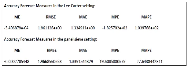
To verify the forecast goodness of the bootstrap technique under consideration, some measures of forecast accuracy can be investigated. There are some commonly used accuracy measures whose scale depends on the scale of the data, like ME, RMSE and MAE, and others scale- independent, like MPE and MAPE. In the following numerical application we offer a comparative implementation of these measures in both the Lee Carter model (where is dependence not assumed) and in the panel sieve algorithm (which considers dependence) to show how the latter improves the accuracy in the mortality forecasts. Moreover, we set out a backtesting procedure for multi-ahead mortality projections (as in Dowd et al. 2010) to evaluate the forecast performance of the bootstrap algorithm.

5. Empirical evidence

Chang (2004) prove the validity of the AR sieve bootstrap in the context of panel data if there is only contemporaneous dependence between units; however, this condition is likely to be violated in many empirical applications. In this section, we verify if the condition of validity of the AR sieve bootstrap in panel data exists for mortality data, in order to apply a bootstrap algorithm to the residuals of the Lee Carter model. In other words, we have to verify if the residuals on which we will operate the bootstrap are distributed as a vector white noise.   ˆ ˆ ˆ ˆ 1 j t x n p j j xt

xt u u

7

We investigate the empirical evidence of the aforementioned condition by considering the Italian male mortality dataset, ranging from 1980 up to 2006, from ages 0 up to 100. The death rates, considered by single calendar year and by single year of age, are aggregated in

an open age group 100+ for the class of age above 100 years. Before implementing the

bootstrap algorithm, we proceed as follows:

1. we fit the Lee Carter model to the selected dataset;

2. we analyze the residuals: as has been well verified in the literature, the independence assumption is violated;

3. we operate an autoregressive approximation of the residuals for each age. We specify the value of the lag length q

 

(1973) and calculate the autoregressive coefficients by using the Yule-Walker method. 4. we verify if the errors of the autoregressive approximation operated in the previous step are a vector white noise.

A k by 1 vector stochastic process

 

 

















k x k s t t k t

E

E

E

'

0

'

0











 

Figure 1 illustrates the evolution of the mortality dynamics over age, simultaneously highlighting the log death rate trends from 1980 to 2006.

Figure 1- log death rates - Italian male population, age: from 0 to 100 (the upper curve represents the year 1980 while the lowest curve shows the rates for 2006)

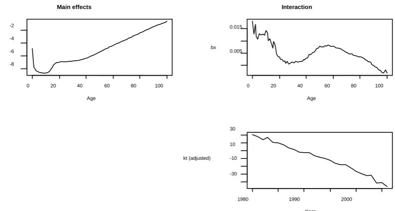
In order to produce mortality death rates projections, we implement the standard version of the Lee Carter model (1992). Figure 2 shows the estimates of the model parameters provided by the demography package developed in R software (Hyndman):

Figure 2- ax, bx, kt adjusted, basic Lee Carter model - Italian male population, age: from 0 to 100

As is shown in Figure 3, there are systematic patterns in the residual plots suggesting that the independence assumption is violated.

Figure 3- Residuals year vs age – basic Lee Carter model -Italian male population, age: from 0 to 100

Starting from the residuals represented, we subdivide the matrix of residuals into n vectors, where n corresponds to the number of ages being considered, and find an autoregressive approximation for the residuals for each age. For the sake of clarity, let us consider the first row vector of the residual matrix which corresponds to the age equal to 0. We represent it as an AR process and calculate the correspondent forecasted errors. We successively replicate the above operation for each row vector (each age) and construct a new matrix of errors, where, in each row, the errors of the AR processes derived exactly from the residuals of the Lee Carter model are allocated. Finally, by verifying if the composed matrix represents a vector white noise, we can check whether the conditions described in formula

 

8

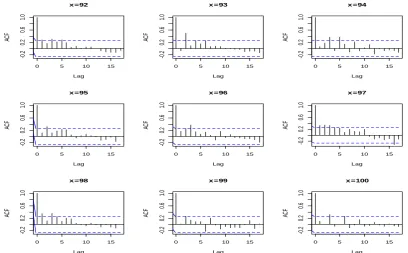
In previous studies, the fitting of the Lee Carter model has been shown and the residuals have been represented, which reveal that there is dependence in the residuals. In the following, we fully investigate the particular dependence structures. Separately for each row and column, respectively representing age and calendar year, we have produced the correlograms shown, in order to highlight graphically the correlation between values of the process at different points in time and at different ages. The first group of correlograms, which is displayed in Figure 4, is constructed considering the correlation between years for each age. In this case, for each age, we are dealing with a time series generated from a stochastic process and verify the autocorrelations over time. In other words, we verify the existence of temporal dependence for each age during the years. The correlograms show the presence of temporal dependence for almost all ages and in particular for the younger ones.

Figure 4- Autocorrelation function of the residuals by age

The second group of correlograms, which is displayed in Figure 5, is constructed by considering the correlation between ages for each year of the dataset. Thus, time 1 corresponds to the year 1980, time t=2 to the year 1981 and so on. They show the persistence of spatial correlation in almost all cases between the years; in other words, in this case, spatial correlation means that there is a dependence structure between ages in the same year and this appears for each year that is separately considered: given t, we observe the correlation between the residuals of age x=0,1,2,…,p where p is the maximum lag considered.

Figure 5 - Autocorrelation function of the residuals by time

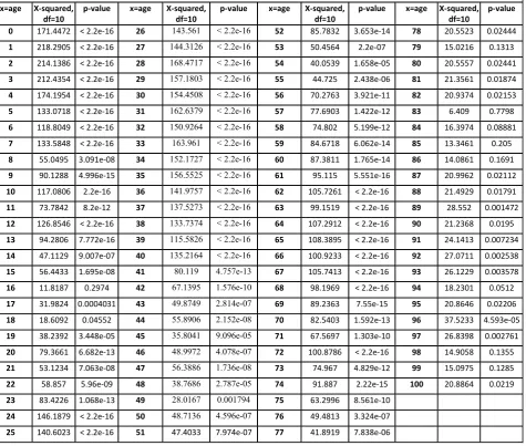
The previous graphical analysis is supported by the results of the Ljung-Box test, which have been implemented for each age separately. As shown in table 1, for almost all ages, the hypothesis of null correlation is rejected. In conclusion, we note that the presence of a dependence structure between residuals of the mortality model has been verified and so needs to be taken into account

.

Table 1 - Ljung-Box test on the residuals

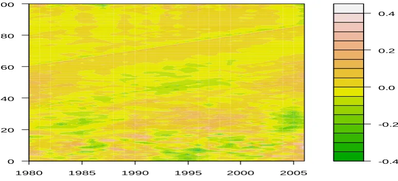
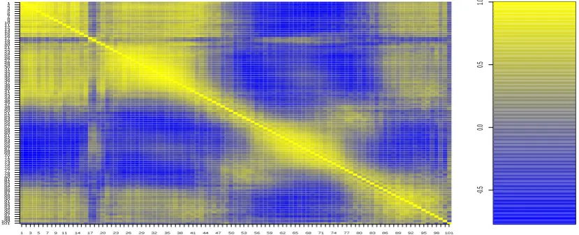
Furthermore, for formally testing the dependence structure into the residuals, we have considered also the standard measure of Pearson, since it is particularly suitable to the configuration model which assumes normality in the residuals. Table 2 and Figure 6 show a strong positive dependence.

Table 2 - Pearson’s correlation coefficient test on the residuals

Figure 6 - Pearson’s correlation coefficient on the residuals - contour map

Thus, the presence of a dependence structure in residuals of the mortality model has been verified and needs to be taken into account.

At this stage we compare two kinds of simulation scheme: a) the residual bootstrap on the Lee Carter residuals relying on the independence assumption; b) the Panel Sieve bootstrap

9

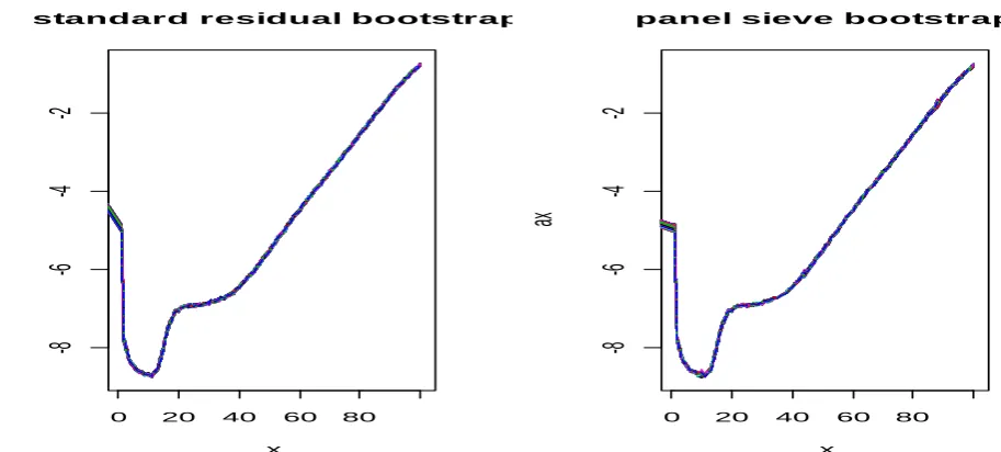
algorithm that we have developed in the Lee Carter setting for capturing the dependence structures which we have assessed. Figures 7-10 display the simulated trajectories for the model parameters for _x, _xand k_tin the two different bootstrap schemes for different numbers of simulations B100,500,1000. The model is fitted to the Italian male mortality dataset, ranging from 1980 up to 2006, from ages 0 up to 100 and then the parameter kt is projected for h=1,...,15 years ahead.

We begin by examining the following Figures which illustrate the simulated patterns for the model parameters for x, xand ktand for the projected ktin the case of B1000

Figure 7 – Simulated paths for ax – Residual Bootstrap and Panel Sieve Bootstrap

Figure 8 - Simulated paths for bx – Residual Bootstrap and Panel Sieve Bootstrap

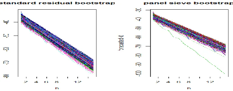
Figure 9 - Simulated paths for kt – Residual Bootstrap and Panel Sieve Bootstrap

Figure 10 - Forecasted kt – Residual Bootstrap and Panel Sieve Bootstrap

As is highlighted in the graphs, the Panel Sieve Bootstrap produces wider confidence

intervals, since it allows for another source of risk: the dependency risk (D’Amato et al.

2012).

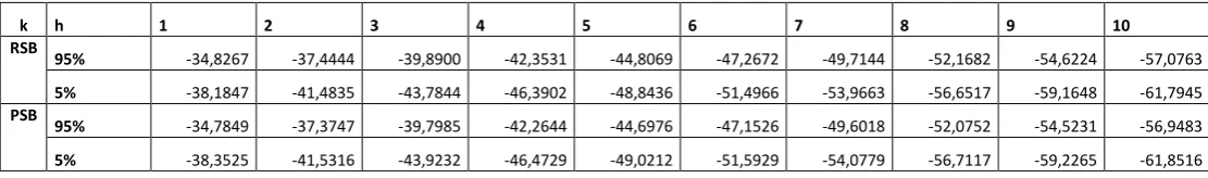
In our analysis, we find the following numerical results on the basis of the algorithm indicated in section 4. Table 3 illustrates different percentiles of the mean of projection of kt

obtained implementing different bootstrap algorithms for future times of valuation equal tohand for the number of simulations equal toB100. In particular, for h1,...,15periods ahead, the performance of the residual bootstrap and panel sieve bootstrap is examined by calculating 5% and 95% confidence intervals, CI’s.

Table 3 – Comparison among Residual Sieve Bootstrap (RSB) and Panel Sieve Bootstrap (PSB), B=100

As is clearly shown by Table 4, if we compare the different algorithms in terms of the distance between the 95% and 5% percentiles, we notice the wider CI’s for the Panel Sieve Bootstrap. From this point of view, the residual bootstrap leads to less uncertain projections, with the dependency in the data being completely neglected. In the case of Panel Sieve bootstrap procedure we are able to capture the whole correlation structure and thereby obtain more reliable projections.

Table 4 – Comparison among Residual Bootstrap and Panel Sieve Bootstrap, in terms of the difference between 95% and 5%, B=100

The outcomes remain stable for the increasing the number of replications, as shown in tables

5-8, for the cases of B500and B1000.

Table 5 – Comparison among Residual Bootstrap and Panel Sieve Bootstrap, B=500

10

Table 6 – Comparison among Residual Bootstrap and Panel Sieve Bootstrap, in terms of the difference between 95% and 5%, B=500

Table 7– Comparison among Residual Bootstrap and Panel Sieve Bootstrap, B=1000

Table 8 – Comparison among Residual Bootstrap and Panel Sieve Bootstrap, in terms of the difference between 95% and 5%, B=1000

To verify the forecast goodness of the panel sieve bootstrap technique, we investigate some measures of forecast accuracy in both Lee Carter model and in the panel sieve algorithm; table 9 shows how the panel sieve bootstrap improves the accuracy in the mortality forecasts with respect to widely used Lee Carter model.

Table 9– Comparison among Lee Carter and Panel Sieve bootstrap in terms of forecast accuracy

Finally, we set out a backtesting procedure for multi-ahead mortality projections to evaluate the forecast performance of the panel sieve bootstrap algorithm. Its implementation is based on the following steps:

- selection of the metric of interest: we have chosen to adopt the life expectancy at birth, which is a very useful metric in the actuarial practice;

- selection of the historical lookback window and the lookforward window to make the backtesting forecasts: we have considered the Italian male mortality dataset, ranging from 1980 up to 1996, from ages 0 up to 100; it is a reduced dataset with respect to that previously used, so that it is possible to produce projections from 1997 to 2006 and compare them with the realized values of the metric of interest.

- graphical results.

Figure 11 – Backtesting on life expectancy in LC and PSB

Figure 11 shows the results of the backtesting procedure; in it we compare the actual expectancy of life at birth, calculated on the realized mortality dataset for an Italian male ranging from 1980 to 2006, with those obtained with a backtesting on the Lee Carter model and the panel sieve boostrap. We observe that, even though both models produce a well- known underestimation of the life expectancy, the projections achieved with the panel sieve bootstrap are closer to the actual values, due to a wider projection interval.

6. Concluding Remarks

The complex structure of the longevity phenomenon means that, in order to produce reliable projections of mortality indices, the interactions between age and time cannot be neglected. Ignoring dependency risk (D’Amato et al. 2012) would lead to an inefficient risk management strategy for insurance companies.

In particular, the presence of spatial dependence across age and time leads to a systematic over-estimation or under-estimation of uncertainty in the estimates, caused by whether negative or positive dependence dominates (Liu et al. 2010).

As is well-known in the demographic literature, the Lee Carter model has become the seminal

statistical model for projections of mortality. To obtain a measurement of the uncertainty in

the forecasted mortality rates, reliable confidence intervals for the quantities of interest connected to the phenomenon under consideration can be calculated on the basis of simulation techniques.

11

Nevertheless, we propose a method which leads to a prudent measure of longevity risk, avoiding the structural incompleteness of the ordinary simulation bootstrap methodology

which involves the assumption of independence. The algorithm that we have studied

combines model-based predictions in Lee Carter framework (1992) with a bootstrap procedure for dependent data, and so both the historical parametric structure and the intra-group error correlation structure are preserved. D’Amato et al. (2012) apply a sieve bootstrap to the residuals of the Lee Carter model, according to the design of the typical autoregressive sieve bootstrap. According to this scheme, we develop a Panel Sieve Bootstrap in the Lee Carter setting, and are able to reproduce in the sampling the dependence structure that exists between the years of the dataset for each age. The methodology is sufficiently flexible to be extended to the whole family of the Lee Carter models in order to take into account additional

issues. In particular one important question is represented by the cohort effect. In this paper,

the benefit of introducing the cohort effect has not been studied, but certainly deserves a deeper investigation. Nevertheless, the method we have proposed, which utilises the basic version of the Lee Carter model, can incorporate a consideration of the cohort effect. In this context, the literature recognises the desirable properties and the good performance of the Renshaw and Haberman (2006) model which incorporates the cohort effect in the Lee Carter model. In this context, the literature recognises the desirable properties and the good performances of the Renshaw and Haberman Lee Carter version (2006) which allows for cohort effect.

Another additional issue to address is the higher variability in the older age groups due to small sample size, that influences the accuracy in the mortality. Hyndman and Ullah (2007) show a particular version of the LC methodology based on the combination of functional data analysis and nonparametric smoothing and D’Amato et al (2011c) offer a comparative analysis of LC and the Hyndman Ullah version. Further analysis could combine smoothing techniques and bootstrap procedure in the mortality setting to improve beyond the forecasts. Future research will focus on detecting the dependence across different populations. The investigation about the factors driving changes in mortality, in particular across countries, requires us to handle the related high dimensional data question. The high dimensionality refers to the total number of data ‘cells’ that are modeled, and this is equal to the product of the numbers of categories for the factors classifying the data.

In order to address the dimensionality problem by extracting age patterns from the data we will take into account principal components approaches in future work.

ACKNOWLEDGEMENTS

The authors would like to express their gratitude to the participants at 9th International Conference

on Computational Management Science whose comments have been extremely useful in helping us to revise a previous version of the present work.

References

Alonso, A. M., Pena D., Romo, J., 2002, Forecasting time series with sieve bootstrap, Journal of

Statistical planning and inference, 100

12

Amemiya, T., 1973, Generalized least square with an estimated autocovariance matrix,

Econometrica, 41, 723-732

Berkowitz, J., Kilian, L., 1996, Recent developments in bootstrapping time series. Econometric

Reviews 19 (1), 1-48

Brouhns N., Denuit M., van Keilegom I., 2005, Bootstrapping the Poisson log-bilinear model for mortality forecasting, Scandinavian Actuarial Journal, 3, 212-224

Bühlmann, P.,1997, Sieve bootstrap for time series. Bernoulli 3, 123-148

Bühlmann, P., 1998, Sieve bootstrap for smoothing in nonstationary time series. Annals of Statistics

26 (1), 48-82

Bühlmann, P., 2002, Bootstrap for time series. Statistical Science 17 (1), 52-72

Chang, Y., 2004, Bootstrap unit root tests in panels with cross-sectional dependency, Journal of

Econometrics, vol. 120(2), pages 263-293.

Choi, E., Hall, P., 2000, Bootstrap confidence regions computed from autoregressions of arbitrary

order, Biometrika, 62: 461-477

D’Amato, V., S. Haberman, M. Russolillo, 2009, Efficient Bootstrap applied to the Poisson Log-Bilinear Lee Carter Model, Applied Stochastic Models and Data Analysis – ASMDA 2009 Selected Paper

D’Amato V., Haberman S., Russolillo M., 2011a, The Stratified Sampling Bootstrap: an algorithm

for forecasting mortality rates in the Poisson Lee Carter setting, Methodology and Computing in

Applied Probability 14 (1) 135-148.

D’Amato V., Di Lorenzo E., Haberman S., Russolillo M., Sibillo M., 2011b, The Poisson

log-bilinear Lee Carter model: Applications of efficient bootstrap methods to annuity analyses, North

American Actuarial Journal 15 (2) 315-333.

D’Amato V., Piscopo G., Russolillo M., 2011c, The mortality of the Italian population: Smoothing

techniques on the Lee Carter Model, The Annals of Applied Statistics,5, (2A), 705–724.

D’Amato, V., S. Haberman, Piscopo, G., M. Russolillo, 2012, Modelling dependent data for longevity projections, Seventh International Longevity Risk and Capital Markets Solutions Conference.

Davidson, R., MacKinnon, J.G., 2005, Bootstrap Methods in Econometrics, Chapter 25 in Palgrave Handbooks of Econometrics: Vol. Econometric Theory, ed. Patterson, K.D. e Mills, T.C., Basingstoke, Palgrave Macmillan, 812-838

Deaton, A. and Paxson C., 2004, Mortality, Income, and Income Inequality Over Time in the Britain and the United States. Technical Report 8534 National Bureau of Economic Research Cambridge, MA: . http://www.nber.org/papers/w8534

Denton, F.T, Feaver C.H., Spencer B.G., 2005, Time series analysis and stochastic forecasting: An

econometric study of mortality and life expectancy, Journal of Population Economics 18:203–227

13

Denuit, M., Dhaene, J., Goovaerts, M.J., & Kaas, R. 2005, Actuarial Theory for Dependent Risks: Measures, Orders and Models. Wiley, New York.

Dowd, K., Cairns, A. J. G., Blake, D. P., Coughlan, G., Epstein, D. and Khalaf-Allah, M., 2010, Backtesting Stochastic Mortality An Ex-Post Evaluation of Multi-Period Ahead-Density Forecasts,

Pension Institute, North American Actuarial Journal, 14, n.3, 280-298.

Efron, B., 1979, Bootstrap methods: another look at the jackknife. Annals of Statistics 7, 1-26.

Efron, B., Tibshirani, R.J., 1986, Bootstrap Methods for Standard Errors, Confidence Intervals, and

Other Measures of Statistical Accuracy, Statistical Science 1, 54-75

Efron, B., Tibshirani, R.J., 1997, An Introduction to the Bootstrap, Chapman & Hall

Hyndman R.J., Ullah S., 2007, Robust forecasting of mortality and fertility rates: a functional data approach, Computational Statistics & Data Analysis, issue 10, 4942-4956.

Hyndman R.J., Demography R package: http://robjhyndman.com/software/demography

International Monetary Fund, 2012, Global Financial Stability Report.

Koissi, M.C., A.F. Shapiro, G. Hognas, 2006, Evaluating and Extending the Lee–Carter Model for

Mortality Forecasting: Bootstrap Confidence Interval. Insurance: Mathematics and Economics 26:

1-20

Kreiss, J.P., 1988, Asymptotic Inference for a Class of Stochastic Processes, Habilitationsschrift, Faculty of Mathematics, University of Hamburg,

Germany

Kreiss J., 1992, Bootstrap procedures for AR(1)-process, Bootstrapping and Related Techniques. Lecture Notes in Economics and Mathematical Systems Springer 376, 107-113

Kreiss J.P., Paparoditis E., Politis D. N., 2011, On the range of validity of the autoregressive sieve

bootstrap, Annals of Statistics 39, 2103–2130.

unsch, H.R., 1989, The jackknife and the bootstrap for general stationary observations, Annals of

Statistics 17 1217-1241.

Lahiri, S.N., 2003, Resampling Methods for Dependent Data, Springer.

Lee, R.D., L. R. Carter, 1992, Modelling and Forecasting U.S. Mortality, Journal of the American Statistical Association, 87, 659-671.

Liu X. and Braun W.J., Investigating Mortality Uncertainty Using the Block Bootstrap, Journal of Probability and Statistics, vol. 2010, Article ID 813583, 15 pages, 2010. doi:10.1155/2010/813583

Palm F. C., 1977, On univariate time series methods and simultaneous equation econometric Models, Journal of Econometrics 5, 379–388.

14

Paparoditis, E., 1992, Modelling Long Term Dependence in Measurement Errors of Plutonium Concentration. Statistical Papers 33, 159-170

Renshaw, A. E., Haberman S., 2006, A Cohort-Based Extension to the Lee-Carter Model for Mortality Reduction Factors, Insurance: Mathematics and Economics 38: 556–70

Renshaw A.E., Haberman S., 2008, On simulation-based approaches to risk measurement in mortality with specific reference to Poisson Lee-Carter modelling. Insurance: Mathematics and Economics 42, 797-816.

Smeeks S., Urbain J.P., (2011), On the Applicability of the Sieve Bootstrap in Time Series Panels, Meteor Research Memorandum, Maastricht University December 2011 (RM/11/055)

Swiss Re, 2011, Longevity risk and protection for Canada.

Trapani, L., 2011, On bootstrapping panel factor series. CEA@Cass Working Paper Series WPCEA04-2011, Cass Business School

Wills S., Sherris M., 2008, Integrating Financial and Demographic Longevity Risk Models: An Australian Model for Financial Applications, Discussion Paper PI-0817.

Figure 1- log death rates - Italian male population, age: from 0 to 100 (the upper curve represents the year 1980 while the lowest curve shows the rates for 2006)

Figure 2- ax, bx, kt adjusted, basic Lee Carter model - Italian male population, age: from 0 to 100

0 20 40 60 80

-8 -6 -4 -2

Italy: male death rates (1980-2006)

Age Log death rate

0 20 40 60 80 100 -8

-6 -4 -2

Main effects

Age ax

0 20 40 60 80 100 0.005

0.015

Age bx

Interaction

Year kt (adjusted)

1980 1990 2000 -30

-0.4 -0.2 0.0 0.2 0.4

1980 1985 1990 1995 2000 2005

0 20 40 60 80 100

Figure 3- Residuals year vs age – basic Lee Carter model -Italian male population, age: from 0 to 100

0 5 10 15

-0 .2 0. 2 0. 6 1. 0 Lag AC F x=1

0 5 10 15

-0 .2 0. 2 0. 6 1. 0 Lag AC F x=2

0 5 10 15

-0 .2 0. 2 0. 6 1. 0 Lag AC F x=3

0 5 10 15

-0 .2 0. 2 0. 6 1. 0 Lag AC F x=4

0 5 10 15

-0 .2 0. 2 0. 6 1. 0 Lag AC F x=5

0 5 10 15

-0 .2 0. 2 0. 6 1. 0 Lag AC F x=6

0 5 10 15

-0 .2 0. 2 0. 6 1. 0 Lag AC F x=7

0 5 10 15

-0 .2 0. 2 0. 6 1. 0 Lag AC F x=8

0 5 10 15

Figure 4- Autocorrelation function of the residuals by age

0 5 10 15 20

-0 .2 0. 2 0. 6 1. 0 Lag AC F t=1

0 5 10 15 20

-0 .2 0. 2 0. 6 1. 0 Lag AC F t=2

0 5 10 15 20

-0 .2 0. 2 0. 6 1. 0 Lag AC F t=3

0 5 10 15 20

-0 .2 0. 2 0. 6 1. 0 Lag AC F t=4

0 5 10 15 20

-0 .2 0. 2 0. 6 1. 0 Lag AC F t=5

0 5 10 15 20

-0 .2 0. 2 0. 6 1. 0 Lag AC F t=6

0 5 10 15 20

-0 .2 0. 2 0. 6 1. 0 Lag AC F t=7

0 5 10 15 20

-0 .2 0. 2 0. 6 1. 0 Lag AC F t=8

0 5 10 15 20

-0 .2 0. 2 0. 6 1. 0 Lag AC F t=9

0 5 10 15

-0 .2 0. 2 0. 6 1. 0 Lag AC F x =92

0 5 10 15

-0 .2 0. 2 0. 6 1. 0 Lag AC F x =93

0 5 10 15

-0 .2 0. 2 0. 6 1. 0 Lag AC F x =94

0 5 10 15

-0 .2 0. 2 0. 6 1. 0 Lag AC F x =95

0 5 10 15

-0 .2 0. 2 0. 6 1. 0 Lag AC F x =96

0 5 10 15

-0 .2 0. 2 0. 6 1. 0 Lag AC F x =97

0 5 10 15

-0 .2 0. 2 0. 6 1. 0 Lag AC F x =98

0 5 10 15

-0 .2 0. 2 0. 6 1. 0 Lag AC F x =99

0 5 10 15

Figure 5 - Autocorrelation function of the residuals by time

Figure 6 - Pearson’s correlation coefficient on the residuals - contour map

1 3 5 7 911 14 17 20 23 26 29 32 35 38 41 44 47 50 53 56 59 62 65 68 71 74 77 80 83 86 89 92 95 98 101 101

1009998 97 96 95 94 93 92 91 90 89 88 87 86 85 84 83 82 81 80 79 78 77 76 75 74 73 72 71 70 69 68 67 66 65 64 63 62 61 60 59 58 57 56 55 54 53 52 51 50 49 48 47 46 45 44 43 42 41 40 39 38 37 36 35 34 33 32 31 30 29 28 27 26 25 24 23 22 21 20 19 18 17 16 15 14 13 12 11 1098 7 6 5 4 3 2 1 -0 .5 0. 0 0. 5 1. 0

0 5 10 15 20

-0 .2 0. 2 0. 6 1. 0 Lag AC F t=48

0 5 10 15 20

-0 .2 0. 2 0. 6 1. 0 Lag AC F t=49

0 5 10 15 20

-0 .2 0. 2 0. 6 1. 0 Lag AC F t=50

0 5 10 15 20

-0 .2 0. 2 0. 6 1. 0 Lag AC F t=51

0 5 10 15 20

-0 .2 0. 2 0. 6 1. 0 Lag AC F t=52

0 5 10 15 20

-0 .2 0. 2 0. 6 1. 0 Lag AC F t=53

0 5 10 15 20

-0 .2 0. 2 0. 6 1. 0 Lag AC F t=54

0 5 10 15 20

-0 .2 0. 2 0. 6 1. 0 Lag AC F t=55

0 5 10 15 20