A conservative bound for the probability of failure of a 1-out-of-2 protection system with one hardware-only and one software-based protection train

City, University of London Institutional Repository

Citation:

Bishop, P. G., Bloomfield, R. E., Littlewood, B., Popov, P. T., Povyakalo, A. A. and Strigini, L. (2014). A conservative bound for the probability of failure of a 1-out-of-2 protection system with one hardware-only and one software-based protection train. Reliability Engineering & System Safety, 130, pp. 61-68. doi: 10.1016/j.ress.2014.04.002

This is the accepted version of the paper.

This version of the publication may differ from the final published

version.

Permanent repository link:

http://openaccess.city.ac.uk/id/eprint/6547/

Link to published version:

http://dx.doi.org/10.1016/j.ress.2014.04.002

Copyright and reuse: City Research Online aims to make research

outputs of City, University of London available to a wider audience.

Copyright and Moral Rights remain with the author(s) and/or copyright

holders. URLs from City Research Online may be freely distributed and

linked to.

City Research Online: http://openaccess.city.ac.uk/ [email protected]

protection system with

one hardware-only and one

software-based protection train

Peter Bishop, Robin Bloomfield, Bev Littlewood

*

_{, Peter Popov, Andrey}

Povyakalo, Lorenzo Strigini

Adelard and Centre for Software Reliability, City University London

Abstract

Redundancy and diversity have long been used as means to obtain high reliability in critical systems. Whilst it is easy to show that, say, a 1-out-of-2 diverse system will be more reliable than each of its two individual “trains”, assessing the actual reliability of such systems can be difficult because the trains cannot be assumed to fail independently. If we cannot claim independence of train failures, the computation of system reliability is difficult, because we would need to know the probability of failure on demand (pfd) for every possible demand. These are unlikely to be known in the case of software. Claims for software often concern its marginal pfd, i.e. average across all possible demands. In this paper we consider the case of a 1-out-of-2 safety protection system in which one train contains software (and hardware), and the other train contains only hardware equipment. We show that a useful upper (i.e. conservative) bound can be obtained for the system pfd using only the unconditional pfd for software together with information about the variation of hardware failure probability across demands, which is likely to be known or estimatable. The worst-case result is obtained by “allocating” software failure probability among demand “classes” so as to maximise system pfd.

Keywords: Software reliability; redundancy and diversity; probability of failure on demand; 1-out-of-2 system; protection system

26.07.2013

* _{Corresponding author. Address: Centre for Software Reliability, City University London,}

1

Introduction

This paper presents an approach for estimating a conservative probability of failure on demand (pfd) that is applicable to a 1-out-of-2 diverse protection system where one of the protection trains is hardware-based and the other is computer-based.

The use of a protection system is an accepted strategy for hazardous industrial processes. The protection system independently monitors the industrial process and if it detects a departure from the safe operational envelope, it initiates some action that overrides the normal control system to place the process in a safe state.

The departure from the safe operational envelope is known as a demand on the protection system. Demands typically arise from different failures within the physical process and control systems. For example, in the nuclear industry, the underlying physical causes of demands on the protection system are known as postulated initiating events (PIE[1]), and the overall plant safety analysis will identify a set of PIEs that represent credible plant failures (such as loss of electrical grid connection or a rupture in the primary coolant circuit). As part of the design process, maximum rates are assigned for each PIE and, to reduce the risk of a PIE that occurs frequently, diverse means are used to detect the departure from normal operation (like temperature and pressure). These are normally implemented in diverse trains of equipment using different types of sensors and with different means of achieving a safe state for the same PIE.

To improve its reliability, a protection train typically also has a high level of internal redundancy to tolerate hardware failure in the sensors, protection logic, actuators and plant components (like valves or pumps). Even so, if sufficient hardware sub-components fail, the train will be unable to respond to the demand triggered by the PIE. Depending on the PIE involved, different sets of hardware components of the protection train need to be able to respond successfully to demands initiated by different PIEs. Typically the hardware probability of failure on demand for a PIE is determined by fault tree analysis [2], where the minimal cutsets of failed sub-components are identified [3] that result in a demand failure. By quantifying and summing the minimal cutsets, the probability of failure per demand for a given PIE can be computed.

2

Terminology and modeling approach

As discussed above, a protection system responds to demands – events that require its intervention. Whether the protection system will respond correctly or will fail on the demand depends on the characteristics of the demand. The protection system may fail – that is, fail to start the required safety action – if, for instance, some hardware component (or redundant combination of components) that is needed to respond correctly is permanently faulty, or suffers a transient fault, at the time of that demand; or due to a design defect in hardware logic or in software. We therefore can also identify a specific demand as a vector of values that together determine the likelihood of any of the protection trains failing:

• since the protection system monitors the values of state variables of the plant (e.g. pressures, temperatures, measures of flows) and may fail or not depending on their values (especially software bugs may depend on the exact values of the data), this vector includes the sequences of values that are read during the demand event;1

• since hardware probabilities of failure are affected by environmental variables (e.g. temperature, humidity, atmospheric pressure, level of electromagnetic radiation, in the various part of the system), these variables are also parts of the vector. Probabilities of hardware failure are usually available for ranges of variables.

The demand is thus a (vector) random variable; processes in the protected plant and its environment determine the times of occurrence of each demand as an event and the value of the demand vector. In what follows we will use just the term “demand” when the meaning “event” or “vector” is clear from the context.

The demand vector includes all variables that have an effect on the success or failure of any part of the system. Thus, for instance, temperature values at a certain sensor in the plant are part of the demand even if only one of the protection trains reads them. But some components of the demand affect more than one protection train. Thus, for instance, an earthquake that affects two protection trains will increase the probability of failure of both, possibly (if the shock is way above their design limits) to 1. Thus we can model common causes of failure via demands which imply high probability of failure for both trains.

This form of modeling has been used in earlier work [4-6] to model in a consistent way failures due both to physical causes and to design, and thus both hardware and software failures. The basic idea here is one of variation of the probability of system failure between different demands, as an explanation for dependence in failure behavior between diverse trains to be used in a fault tolerant system (e.g. a 1-out-of-2

1 _{With software, one could imagine the protection sytem as realising a deterministic function of the}

system). The idea is a simple one. The probability of a system failing on a demand will, in general, vary across demands. Since the component values of the demand vector together determine the likelihood of a protection train failing, and if the system’s design is such that we can exclude failures of one train directly causing failures of the other, the failures of both trains on a specific demand (a specific value of the demand vector) can be assumed independent conditionally on the demand Interest then centers upon the covariance (across all demands) between the two functions (of the demand) that describe the probabilities of failure of the two trains of a 1-out-of-2 system. When there is positive covariance – roughly, when the demands that associated with a higher probability of failure for one train also tend to to assocviate with a higher probability of failure for the other – then it is more likely that there will be positive correlation between the trains’ failures on a random demand. In such a case, wrongly assuming independence of failures between the two trains will give an optimistic estimate of the reliability of the 1-out-of-2 system2_.

An achievement of these conceptual models is their establishment of, and explanation for, the inevitability of dependence (positive or negative) of failure behavior between redundant, diverse systems, hardware or software. They thus support the empirical evidence for such dependence that comes, for example, from experiments: see e.g. [7, 8]. No longer is it possible to claim that the two diverse protection trains of a 1-out-of-2 fault tolerant architecture will fail independently of one another, without making very strong claims: essentially that there is no variation of failure probability across demands for at least one of the trains. This means that the simple arithmetic of independence is not applicable for the computation of the system reliability as a function of the component reliabilities. Specifically, the pfd of a 1-out-of-2 system over all demands cannot simply be assumed to be the product of the pfds of the two trains. Informally, it means that we need to know how dependent the failures of the trains will be.

Reliability estimation of such a 1-out-of-2 system is non-trivial as it seems to require a complete knowledge of how the probability of failure varies between demands. However, we can reason by failure classes, defining a “class” as a set of demands such that the estimated pfd is the same for all demands in a class. For simple hardware, a “class” means a set of demands such that correct response to any of them requires the same set of subsystems to function correctly. If the demand classes for two protection trains do not exactly coincide, a demand class is defined as a set of demands such that each one of the trains has constant pfd over all the demands in the set. This will generally involve more demand classes for the system than would be defined for each train alone. If this definition led to too many classes of demands, their number can be contained, and kept tractable, by merging classes and using the highest pfd among those classes thus merged. It can easily be shown that given conditional independence on each demand, and constant pfd across the class for at least one of the two trains, failures of the two trains are conditionally independent

2 _{It is possible to do better than independence if there is negative association between the probabilities}

conditionally on the demand class [9]. Thus, the system pfd conditional on a certain demand class is obtained by multiplying the pfd values, for that demand class, of the two trains.

For software, things seem much more problematic: software faults are such that among two demands that are from all other viewpoints in the same “class”, the software may fail on one but not the other depending on the values of the inputs to the software. In fact, claims about software reliability are often limited to the marginal probability of failure on demand based on arguments of quality of production and verification, “proven in use” arguments, or operational testing that is sufficient for assessing marginal pfd but insufficient for assessing conditional pfd for each demand class.

Since independence of failures is not plausible, system pfd depends on how the software pfd varies across demands, or demand classes: a claim of even very low marginal software pfd may not be sufficient to support a claim for satisfactory system pfd. In this paper we derive a worst-case bound on the system pfd given this kind of scenario. We present a solution for deriving a conservative estimate for the system pfd for a 1-out-of-2 protection system architecture where there is software in one train only. The pessimistic (but attainable) bound for the probability of failure on demand for such a system requires only the marginal pfd of the software (together with the varying hardware pfds across different demand classes). The basic ideas here can be generalized to more complex systems than the example we use in the paper.

3

Protection System Reliability Model

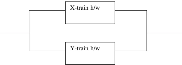
The example 1-out-of-2 system we shall use for illustrating our reliability modeling approach is a nuclear reactor protection system with two trains: the X-train and the Y-train. Real-life examples of such systems include the UK Sizewell B reactor’s primary and secondary protection systems, and the safety systems of advanced gas-cooled reactors (AGRs).

hardware pfd is primarily determined by the minimum equipment requirement for the specific demand class rather than the state of the reactor.

X-train h/w

[image:7.595.153.443.130.234.2]

Y-train h/w

Figure 1. Independent trains (hardware based)

Conditional on each demand class there is conditional independence between failures of the X and Y trains. This assumption is justified on the basis of there being effective isolation between the trains, to avoid failure propagation between them, and there being no variation of pfd for the hardware of a train between demands within a demand class. Common stresses (e.g. like elevated temperatures) or shocks are modeled as creating specific demand classes where hardware pfds are increased, but still failures are independent conditional on this higher pfd (possibly very close to 1, for shocks affecting hardware in both trains) [5].

With these assumptions, we can see that the (marginal) probability of failure on demand of the 1-out-of-2 system, i.e. for a randomly chosen demand, is the probability of both X-train hardware and Y-train hardware failure:

) ( ) ( )

(i p i f i p

pfd

h h h

h Y

i X Y

X =

∑

(1)

where p (i)

h

X is the probability of X-train hardware failure on demand class i, pY_h(i)

is the probability of Y-train hardware failure on demand class i, and _f(i) is the probability that a randomly chosen demand is of class i.

Clearly, the pfd is different from the result that would be obtained under an incorrect assumption of unconditional independence of failure between the two trains, which is

   

     

 

=

∑

∑

i Y i

X Y

X pfd p i f i p i f i

pfd

h h

h

h. ( ) () ( ) ()

The true result will exceed the incorrect result (based on the false assumption of independence) so long as there is positive covariance between the X- and Y-train demand class pfds, p (i)

h

X and pY_h(i). This is similar to the result that Eckhardt and

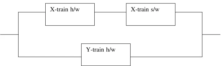
We now consider the situation that is the subject of this paper, in which one train contains software, and the train fails if the software fails: see Fig 2.

We still classify the demands into classes with constant hardware pfd as before. There is still conditional independence, conditional on the demand class, between failures of the X-train (hardware and software), on the one hand, and the Y-train (hardware only) on the other, for each demand class i. This is because (i) the trains fail independently conditional on each demand; and (ii) within each demand class, the pfd of train Y is the same for every demand. Thus the probability of failure on demand is now:

(

p (i) p (i) p (i)

)

p (i)f(i) pfd

h s h s

h h

s

h Y

i

X X

X Y

X + =

∑

+ − + . (2)

where p (i)

s

X is the probability of failure of the X-train software on a demand of

class i and p (i)

s h

X ₊ is the probability of simultaneous hardware and software failure

on a demand of class i.

X-train h/w

Y-train h/w

[image:8.595.137.493.364.471.2]

X-train s/w

Figure 2. Hardware train plus computerized train

To use expression (2) we need to know, or more plausibly, be able to estimate, the parameters on the right hand side.

In many cases it is likely that estimates of

{

p (i)

}

h

X ,

{

pYh(i)

}

could be based on

knowledge of the different subsets of hardware required for each demand class. The parameters

{

p (i)

}

s h

X+ are not likely to be known, nor to be estimatable, but it is clearly

conservative to set them to 0.

The major practical difficulty is that the

{

p (i)

}

s

X will generally be unknown and not

estimatable. However, an estimate of

s

X

pfd , the marginal pfd of the X-train software, will often be available, based on the usual qualitative criteria used for claims about software, or possibly on operating experience in other similar contexts.

4

Worst case system

pfd

Firstly, it is easy to see that, for given values of the known parameters, the largest value of the system pfd, (2), occurs when ( )=0

+ i

p

s h

X for all i. This conservative

bound on the system pfd is then

) ( ) ( )

(i p i f i p

pfd pfd

h s h

h h

s

h Y

i X Y

X Y

X ₊ = +

∑

(3)

Secondly, we need to know what is the worst allocation of the marginal pfd of the X-train software to the second term on the right hand side of (3), i.e. the one that makes (3) the largest value that this conservative bound on the system pfd can take. That is, we need to find which set of numbers

{

p (i)

}

s

X , satisfying the constraint

∑

= i

X

X p i f i

pfd

s

s () (), maximizes

∑

i

Y X i p i f i

p

h

s( ) ( ) ( ).

Now

(

( ), ()

)

(

( )

) (

( )

)

) ( ) ( )

(i p i f i Cov p i p i E p i E p i p

h s

h s h

s X Y X Y

i

Y

X = +

∑

where E

(

p (i)

)

s

X is the marginal pfd of the software, i.e. =

∑

i

X

X p i f i

pfd

s

s () ( ), and

(

p (i)

)

E

h

Y is the marginal pfd of the Y-train hardware, i.e. pfd p (i)f(i) i

Y

Y_h =

∑

_h . If we

keep these two probabilities constant, the maximum value of

∑

i

Y X i p i f i

p

h

s( ) ( ) ()

occurs when Cov

(

p (i),p (i)

)

h

s Y

X takes its maximum value. Clearly this occurs when

we associate large values of p (i)

s

X with large values of pYh(i).

We call the allocation process “bin-filling”. Informally, we proceed by first allocating as much of

s

X

pfd as we can to the demand “bin” that has maximum Y-train hardware pfd; we allocate as much of the remaining

s

X

pfd to the demand bin with the next largest Y-train hardware pdf, and so on until we have ‘used up’ all of

s

X

pfd . In each allocation of part of

s

X

pfd to a demand class, we recall that in this conservative case we have assumed that hardware and software failures are disjoint for all demand classes: thus only enough of

s

X

pfd is allocated to a demand class to make failure of this class certain (i.e. from either a hardware or a software failure).

Without loss of generality, we can order the demand bins, i, by their Y-train pfd, such that p (i)≥ p (i+1)

h

h Y

Y

We define a term S(i) as the software pfd that is available for allocation to bin i. So we start with:

s

X pfd S(1)=

Then, starting at i=1, we assign:

   

 

− =

) (

) ( ), ( 1 min ) (

i f

i S i p i

p

h

s X

X

The software pfd remaining for the next bin is:

) ( ) ( ) ( ) 1

(i S i f i p i S

s

X

− =

+

This process continues up to bin j, say, where the software pfd has been used up, i.e. where S(j+1)=0

The final bin j may, of course, not be completely filled (i.e. the probability of failure associated with the bin – from hardware and software – may be less than 1).

As S(j+1)=0, all remaining bins will be assigned a software failure probability of zero.

The numbers

{

p (i)

}

s

X that result from this procedure give the worst case value for the

conservative system pfd bound (3). A precise statement of this result, and its proof, can be found in the Appendix.

One way of using this result is to compare it with a naïve estimate that ignores variations in software pfd across demand classes, i.e. where we assume that the marginal software pfd is applied to all demand classes The difference can be expressed as a ratio of the pfd obtained using the worst-case

{

p (i)

}

s

X values, and

using

s

s X

X i pfd

p ( )≡ .

5

Examples

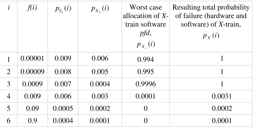
Informally, the theorem states that the worst case error (i.e. the maximum underestimate of the system pfd) will occur when all the X-train software pfd is associated “parsimoniously” with those demand classes that have the largest Y-train hardware pfds. Consider the (artificial) example in Table 1.

the question is how to allocate the X-train software failure probabilities to maximize the underestimate of system pfd, subject only to constraining the X-train marginal software pfd to be 0.001.

In the table, the Y-train hardware pfds have been ranked in descending order of magnitude. We assign just sufficient X-train software pfd to each of the largest of the Y-train hardware pfds to make X-train failure (from either hardware or software) certain for these demand classes. We can do this for demand classes 1, 2, 3; but there is not sufficient X-train software pfd remaining to do it for demand class 4. In fact, demand class 4 has a software pfd of 0.0001 in order to satisfy the constraint that the marginal X-train software pfd over all demand classes is 0.001. That is:

001 . 0 ) 4 ( ) 4 ( ) ( ) (

3

1

= ⋅ +

=

∑

=

i

X X

X f i p i p f

P

s s

s

The overall probability of X-train failure – from hardware or software – for demand class 4 is then 0.0031. For the remaining demand classes, 5 and 6, software failure is impossible under this assignment – all the X train software pfd has been “used up” on the earlier demand classes – although hardware failure is possible: see last two entries in final column of Table 1.

i f(i) p (i)

h

Y pX_h(i) Worst case

allocation of X-train software

pfd,

) (i p

s

X

Resulting total probability of failure (hardware and

software) of X-train, )

(i pX

1 0.00001 0.009 0.006 0.994 1

2 0.00009 0.008 0.005 0.995 1

3 0.0009 0.007 0.0004 0.9996 1

4 0.009 0.006 0.003 0.0001 0.0031

5 0.09 0.0005 0.0002 0 0.0002

[image:11.595.90.502.398.606.2]

6 0.9 0.0004 0.0001 0 0.0001

Table 1. Bin filling example

It can be seen that the binning procedure allocates zero software pfd to demand classes 5 and 6. This does not mean we postulate the software will actually be perfect for that demand class - it is merely a result of the _{fact that the conservative allocation}

process is designed to maximize the system pfd over all demands.

late entries of the 5th column of the Table, corresponding to the smallest Y-train hardware pfds. There will be at most one row that does not have a 0 in the 5th column, or a 1 in the 6th column: the values of these two entries will be determined by the need to satisfy the constraint.

The pfd of the 1-out-of-2 system, using the worst-case allocation of the X-train as in the fifth column of Table 1, is

(

)

6

10 32 . 7 ) ( ) ( ) ( )

( + = × −

∑

p i p i p i f i

h s

h Y

i

X

X .

In contrast, the system pfd based on assuming (wrongly) that the marginal X-train software pfd, =0.001

s

X

p , applies to all demand classes, is

(

)

7

10 80 . 6 ) ( ) ( 001 . 0 )

( + = × −

∑

p i p i f i

h

h Y

i

X .

Therefore the naïve estimate of system pfd ignoring variation in software pfd between demand classes and the worst case estimate of the system pfd differ by a factor of 10.76.

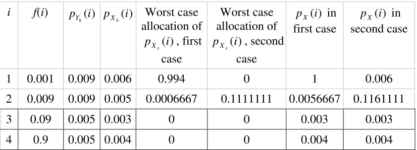
This simple procedure outlined above for obtaining the worst case bound is easy to prove in a case like that in Table 1, where the Y-train hardware pfds are strictly ordered. If, on the other hand, some of the Y-train hardware pfds are identical, there is a complication: in such cases there may be more than one maximum. This can be seen in the example of Table 2 below.

i f(i) p (i)

h

Y pXh(i) Worst case

allocation of ) (i p

s

X , first

case

Worst case allocation of

) (i p

s

X , second

case

) (i pX in

first case

) (i pX in

second case

1 0.001 0.009 0.006 0.994 0 1 0.006 2 0.009 0.009 0.005 0.0006667 0.1111111 0.0056667 0.1161111

3 0.09 0.005 0.003 0 0 0.003 0.003

[image:12.595.90.503.466.615.2]

4 0.9 0.005 0.004 0 0 0.004 0.004

Table 2. Example with a non-unique bin-filling sequence

underestimate of system pfd arising from ignoring variation in X-train software pfd is the same – 0.40×10-5 – in each case.

It can be shown that this will always be true: when there are several ways of worst case allocation of the X-train software pfds, each will give the same maximum underestimate of system pfd.

6

Discussion

The work by Eckhardt and Lee (and later work) introduced a new way of looking at the reasons for dependence between the failure behavior of diverse versions of software. In these models, everything turns on the variation of the failure probability as a function of the specific demand. This earlier work gave novel insights into the reasons why claims for independence are rarely supportable. Unfortunately, it also introduced some serious difficulties for anyone wishing to exploit the models to estimate the actual probabilities of failure of real systems, since this requires estimation of how failure probability varies across all demands.

In this paper we have looked at a particular system: a 1-out-of-2 system in which only one train contains software. In the example that motivated this work – a protection system for a nuclear reactor – we were able to identify a small number of demand classes (<20) for each of which a hardware pfd could be estimated. In fact these had been estimated as part of the wider safety case for the reactor. For software, on the other hand, only a marginal pfd was estimated. Our aim, therefore, was to obtain a means of computing the worst system pfd that could result for a given software marginal pfd. Such a result could be used conservatively as part of a safety case claim.

Our main result, then, is a procedure for finding such a worst case result, based upon a conservative bound on the system pfd which assumes that simultaneous hardware and software failure in a train is impossible.

As we have found elsewhere whilst working on these models of diversity, these results are quite surprising and subtle: witness, for example, the pivotal role played by variation in Y-train hardware pfd when we take into account X-train software failures. We do not think that these results could have been obtained without the formal model of diversity, although we believe that they are intuitively convincing in retrospect.

train pfd, which is at worst min

(

PY_h,PX_h+PX_s

)

. Our tighter result will often be much

lower than this worst case – informally this is because p_Y

h(i)<<1 for all i – although

we can contrive scenarios, with typically implausible values of the parameters, in which it approaches or even equals it.

On the other hand, estimates of software pfd per demand class would allow even tighter estimates of system pfd, which could be orders of magnitude lower if all these

) (i p

s

X are orders of magnitude lower than 1. One way of reading our result is that it

is far better to bring to the calculation of system pfd some estimate of software pfd per demand class, as argued for instance in [10] and exemplified in [9], rather than over the whole demand space. But when the latter is the only estimate available for software pfd, we offer a way of using other knowledge that is available per demand class to avoid extreme overestimation of system pfd.

These results depend on the ability to state estimates of constant pfd per demand class on the Y channel, that is, to trust that the Y channel is free from demand-specific variation of pfd within a demand class. If this could not be assumed (for instance if Y implemented complex logic - albeit hard-wired - that were not trusted free of design faults affecting specific demands in one class), a more conservative method suitable for two software-based trains (e.g. as [9]) should be used.

Note that, if a conservative value of the X-train software pfd over all demand classes were available (i.e. a value that is not exceeded by its true pfd on any demand class), then the system pfd calculated using this value for all the p (i)

s h

X + terms in expression

(2) would be conservative. In fact, it may be very conservative: our result points to a way of lessening this conservatism.

Acknowledgement

Support for the work reported here came from:

• the UnCoDe (Uncertainty and confidence in safety arguments) project, funded by the Leverhulme Trust;

References

[1] Introduction to the Safety, Security and Environmental Report (SSER).Documernt reference UKEPR-0001-001 Issue 06. UK Office for Nuclear Regulation.

[2] Lee W, Grosh D, Tillman F, Lie C. Fault Tree Analysis, Methods, and Applications - A Review. IEEE Trans Reliability. 1985;R-34 194-203.

[3] Nakashima K, Hattori Y. An efficient bottom-up algorithm for enumerating minimal cut sets of fault trees. IEEE Trans Reliability. 1979:353 -7

[4] Littlewood B, Miller DR. Conceptual Modelling of Coincident Failures in Multi-Version Software. IEEE Trans on Software Engineering. 1989;15:1596-614.

[5] Hughes RP. A new approach to common cause failure. Reliability Engineering. 1987;17:211-36.

[6] Eckhardt DE, Lee LD. A Theoretical Basis of Multiversion Software Subject to Coincident Errors. IEEE Trans on Software Engineering. 1985;11:1511-7.

[7] Eckhardt DE, Caglayan AK, Knight JC, Lee LD, McAllister DF, Vouk MA, et al. An experimental evaluation of software redundancy as a strategy for improving reliability. IEEE Trans Software Eng. 1991;17:692-702.

[8] Knight JC, Leveson NG. Experimental evaluation of the assumption of independence in multiversion software. IEEE Trans Software Engineering. 1986;12:96-109.

[9] Popov P, Strigini L, May J, Kuball S. Estimating Bounds on the Reliability of Diverse Systems. IEEE TSE. 2003;SE-29:345-59.

Appendix: Worst case value for the conservative system

pfd

bound

We need to find the set of numbers

{

p (i)

}

s

X , satisfying the constraints:

n i i p i f i p pfd s s s X n i X X .. 1 , 1 ) ( 0 ; ) ( ) ( 1 = ≤ ≤ =

∑

= (A1) that maximizes

(

( ) ( ) ( )

)

() ( ) 1 i f i p i p i p i p pfd h s h s h h s h Y n i X X X Y X

∑

= +

+ = + − , (A2)

where n is the number of demand bins; p (i)

s

X is the probability of failure of the

X-train software on a demand of class i, and p (i)

s h

X + is the probability of simultaneous

hardware and software failure on a demand of class i.

We assume that the X-train software and hardware are reliable enough to satisfy

, 1 ≤ + h S X X pfd pfd

i.e. the failures of the X-train software and hardware can be mutually exclusive. The conservative bound for (A2) is

(

)

) ( ) ( )) ( 1 ), ( min( ) ( ) ( )) ( 1 ), ( min( ) ( 1 1 i f i p i p i p pfd i f i p i p i p i p pfd h h s h h h h s h h s h Y n i X X Y X Y n i X X X Y X

∑

∑

= = − + = − + = +

Thus, we need to find the set of numbers

{

p (i)

}

s

X , satisfying the constraints (A1), that

maximizes

∑

= − = n i Y X

X i p i p i f i p E h h s 1 ) ( ) ( )) ( 1 ), (

min( . (A3)

Theorem

If the set of numbers

{

p (i)

}

s

X satisfies the constraints (A1) and:

- without any loss of generality, the bins are ordered in the following way:

) ( ... ) 2 ( ) 1

( p p n

p

h h

h Y Y

- + ≤1

h

S X

X pfd

pfd , i.e.

∑

∑

= = − = − ≤ = n i X X n i X

X p i f i pfd p i f i

pfd h h s s 1 1 ) ( )) ( 1 ( 1 ) ( )

( ; (A4)

- integer number k satisfies: 1 ≤ k ≤ n and

∑

∑

= − = − ≤ ≤ − k i X X k i

X_h pfd _s f i p _h p i f 1 1 1 ) 1 )( ( ) 1 )( ( , then       − − + − = ≤

∑

∑

− = − = 1 1 1 1 )) ( 1 )( ( ) ( ) ( )) ( 1 )( ( ' k i X X Y k i Y

X i p i p k pfd f i p i

p i f E E h s h h h (A5)

Proof

Our proof of the theorem is based upon two lemmas:

Lemma 1

If (A1) and (A4) are satisfied and

{

p (i)

}

s

X is a set of numbers maximising (A3), then

, : 1 ), ( 1 ) (

0 p i p i i n

h

s X

X ≤ − =

≤ (A6) And

∑

= = n i Y X i p i f i p E h s 1 ). ( ) ( )

( (A7)

Proof of Lemma 1

Reductio ad absurdum: let us assume that Lemma 1 is wrong and that for some bin k:

) ( 1 )

(k p k

p

h

s X

X > − . (A8)

The condition (A4) implies that for some other bin l:

) ( 1 )

(l p l p

h

s X

X < − . (A9)

If we consider the new set of numbers

{

}

s

X

p* :

. ) ( ) ( * ; ) ( ) ( * ; and ), ( ) ( * 2 1

δ

δ

+ = − = ≠ ≠ = l p l p k p k p l i k i i p i p s s s s s s X X X X X X (A11)

Then, (A10) and (A11) implies

∑

∑

∑

= ≠ ≠ = = = + + + − = n i X X n l i k i X X X n i X s s S s s s pfd i p i f i p i f l f l p l f k f k p k f i p i f 1 2 1 1 * ) ( ) ( ) ( ) ( ) ( ) ( ) ( ) ( ) ( ) ( ) ( ) (

δ

δ

(A12) and

∑

∑

∑

∑

= = ≠ ≠ = − = > + − = − + + + − = − = n i X X Y Y n i X X Y n l i k i X X Y X Y X Y n i X X Y i p i p i p i f E l p l f i p i p i p i f i p i p i p i f l p l p l f k p k p k f i p p i p i f E s h h h s h h s h h s h h h s h h 1 2 1 2 1 )) ( ), ( 1 min( ) ( ) ( ) ( ) ( )) ( ), ( 1 min( ) ( ) ( )) ( ), ( 1 min( ) ( ) ( ) ) ( )( ( ) ( )) ( 1 )( ( ) ( )) ( * , 1 min( ) ( ) ( * δ δ (A13)

Together, (A12) and (A13) contradict the original premise that the set of probabilities

{

p (i)

}

s

X maximises (A3).

Hence, Lemma 1 is correct.

QED

Lemma 2

If:

- (A1) and (A4) are satisfied;

- the set of numbers

{

p (i)

}

s

X maximizes (A7);

, : 1 )), ( 1 /( ) ( ) ( ' ; : 1 )), ( 1 )( ( ) ( ' n i i p i p i p n i i p i f i f h s s h X X X X = − = = − = (A14)

then the set of numbers

{

p' (i)

}

s

X maximises

∑

= = n i X Y i p i p i f E s h 0 ), ( ' ) ( ) ( ' (A15) given

∑

= = = ≤ ≤ n i X X X s s s pfd i p i f n i i p 1 ) ( ' ) ( ' : 1 , 1 ) ( ' 0 (A16)

If, in addition, without any loss of generality, the bins are ordered in the following way: ) ( ... ) 2 ( ) 1

( p p n

p

h h

h Y Y

Y ≥ ≥ ≥

and integer number k satisfies 1≤ k ≤ n and

∑

∑

= − = ≤ ≤ k i X k i i f pfd i f s 1 1 1 ) ( ' ) (

' then

      − + = ≤

∑

∑

− = − = 1 1 1 1 ) ( ' ) ( ) ( ) ( ' ' k i X Y k i

Y i p k pfd f i

p i f E E s h

h . (A17)

Proof of Lemma 2

The proof of Lemma 2 essentially involves the solution of the following linear programming problem:

Maximise E =

∑

=

n

i

Y

X i p i f i p h s 1 ) ( ' ) ( ) ( '

subject to the constraints

∑

= = n i X

X p i f i

pfd s s 1 ) ( ' ) (

' ; p i i n

s

X () 0, 1..

'

1≥ ≥ = .

The proof of Lemma 2 is in three parts. We need to show:

• that the allocation of X-train software pfd outlined above is necessary;

• that it is sufficient (i.e. that the different allocations, when these are possible, give the same value for the bound);

Proof of necessity

We need to show that, if p i n

s

X (),1 1,...,

' = , is an optimal solution of the above problem, then 0 ) ( ' 1 ) ( ' = ∨ = ⇒

< j p i p j

i

s

s X

X

Informally, the statement means that the components of the optimal solution are in descending order and only one component may have a value different from 1 or 0. In other words, the optimum solution has the following form:

1, ... 1, z, 0, 0, ...,0,

where z satisfies 0≤z≤1.

We start by assuming that the opposite statement is true, i. e.p i i n

s

x ( ), 1..

' = , is an optimal solution of the above problem, but

0 ) ( ' 1 ) ( ' ≠ ∧ ≠ ∧

< j p i p j

i

s

s X

X .

Consider the following new solution:

. 0 ; 0 ; 0 ) ( ' ) ( '' ; 1 ) ( ' ) ( '' ; ), ( ' ) ( '' ; .. 1 ), ( '' ≥ ∆ ≥ ∆ ≥ ∆ − = ≤ ∆ + = ≠ ∧ ≠ = = j i j X X i X X X X X j p j p i p i p j l i l l p l p n k k p s s s s s s s

The value of E implied by the new solution will be

∑

= = n i Y

X i p i f i p E h s 1 ). ( ' ) ( ) ( '' ''

To satisfy the constraints we require )

( ' )

(

' i f j

f _j

i⋅ =∆ ⋅ ∆ That is 0 ) ( ' ) ( ' −∆ ⋅ = ⋅

∆i f i j f j

So, we have

because ) ( )

(i p j p

h

h Y

Y ≥

due to the initial assumption and problem formulation. This means that E≤E '', i. e. the new solution provides a greater value of the objective function and so the initial solution is not optimal. This contradicts the initial assumption, and the proof follows.

Proof of sufficiency

We need to show that a solution of the following kind is an optimal one:

To prove the statement we shall show that the above solution satisfies the optimum criteria for the simplex method [1].

In the standard form [1] the problem is

subject to the equality constraints:

Here: pfd p i f i i n

h S Y

X , (), '( ), =1.. are the problem parameters we defined earlier in

equations (A1) and (A14); z(i), i=1..n are the slack variables [1]. For the considered solution the variables p' (i)

s

X , i=1..k are basic variables [1]. Expressing these basic

variables through non-basic ones:

∑

=

n

i

Y

X i p i f i

p

h S

1

), ( ' ) ( ) ( ' Maximise

. 0 ) (

; 0 ) ( '

; .. 1 , 1 ) ( ) ( '

; )

( ' ) ( '

1

≥ ≥

= =

+

=

∑

=

i z

i p

n i i

z i p

pfd i

f i p

s s

s s

X X n

i

X X

. .. ) 1 ( , 0 ) ( '

; ) ( '

) ( ' )

( '

); 1 ..( 1 , 1 ) ( '

; 1

) (

1

1

n k i i p

k f

i f pfd

k p

k i i p

n k k

S

s S

S

X

k

i X

X X

+ = =

− =

− = = ≤ ≤ ∃

∑

−

, ) ( ' ) ( ' ) ( ' ) ( ' )) ( 1 ( ) ( ' ); 1 ..( 1 ), ( 1 ) ( ' 1 1 1 k f i f i p i f i z pfd k p k i i z i p k i n k i X X X X s s s s

∑

−

∑

= = + − − − = − = − =

The objective function in terms of non-basic variables only is then:

∑

∑

∑

∑

∑

∑

− = = + + = − = − = = + − + − − + = + − − − + − 1 1 1 1 1 1 1 1 1 )) ( ) ( )( ( ' ) ( ' )) ( ) ( )( ( ' )) ( 1 ( ) ( ) ( ' ) ( ) ( ' ) ( )] ( ' ) ( ' ) ( ' )) ( 1 ( [ ) ( ' ) ( )) ( 1 ( k i n k i Y Y X Y Y Y X n k i Y X k i k i n k i Y X X Y k p i p i f i p k p i p i f i z k p pfd i f i p i p k p i f i p i f i z pfd i f i p i z h h s h h h s h s h s s h

We can now write the expression for the reduced cost (i.e. for that part of the objective function value which depends upon non-basic variables):

∑

−

∑

= = + − + − 1 1 1 )) ( ) ( )( ( ' ) ( ' )) ( ) ( )( ( ' ) ( k i n k i Y Y X Y

Y k p i p i f i p i p k

p i f i z h h s h h Since , ).. 1 ( ), ( ) ( ); 1 ..( 1 ), ( ) ( ; .. 1 , 0 ) ( ' n k i k p i p k i k p i p n i i f h h h h Y Y Y Y + = ≤ − = ≥ = ≥

it follows that all coefficients of the reduced cost are negative. Thus an increase in any non-basic variable will decrease the objective function. Hence, the considered solution satisfies the optimum criterion for the simplex method [1]. Hence, the considered solution is optimal.

Proof of value of worst case bound

We now need to show that if

0 ) ( ... ) 2 ( ) 1 (

1≥ p ≥ p ≥ ≥ p n ≥

h h

h Y Y

Y and

∑

−

∑

= = ≤ ≤ ∧ ≤ ≤ ∃ 1 1 1 ), ( ' ) ( ' 1 ) ( k i k i

X f i

pfd i f n k k s then

∑

−

∑

= − = − + = 1 1 1 1 ). ( )) ( ' ( ) ( ' ) ( = ' of Maximum k i k i Y X

Y i f i pfd f i p k

We know that the maximum of E occurs with the following choice of

{

}

s

X p' :

. ).. 1 ( , 0 ) ( ' ; 1 0 ) ( ' ); 1 ..( 1 , 1 ) ( ' ) ( n k i i p z z k p k i i p k s s s X X X + = = ≤ ≤ ∧ = − = = ∃

Thus, from the constraint on unconditional X-train software pfd:

. 1 0 ), ( ' ) ( ' ) ( ' ) ( ' 1 1 1 ≤ ≤ + = =

∑

∑

= − = z k zf i f i f i p pfd n i k i X

X_{s s}

This implies ). ( ) ) ( ' ( ) ( ' ) ( ) ( ' ) ( . ) ( ' ) ( ' ) ( ' ) ( ) ( ' ) ( ) ( ' ) ( ) ( ' ) ( ) ( ' ' E ; ) ( ' ) ( ' ; ) ( ' ) ( ' 1 1 1 1 1 1 1 1 1 1 1 1 1 1 1 1 k p i f pfd i f i p k f k p k f i f pfd i f i p k f k zp i f i p i f i p i p k f i f pfd z i f pfd i f h s h h s h h h h s s s Y k i X k i Y Y k i k i X Y n i k i Y Y Y X k i X k i k i X

∑

∑

∑

∑

∑

∑

∑

∑

∑

− = − = − = − = = − = − = − = = − + = − + = = + = = − = ≤ ≤

and Lemma 2 follows

The main theorem follows if we apply a substitution inverse to (A14) to the upper bound (A17) finally obtaining the constrains (A4) and the upper bound (A5). QED

Reference